$SU(3)/SU(2)$: the simplest Wess-Zumino-Witten term

Abstract

The observation that $SU(3)/SU(2)\cong S^{5}$ implies the existence of a particularly simple quantized topological action, or Wess-Zumino-Witten (WZW) term. This action plays an important role in anomaly cancellation in extensions of the Standard Model electroweak sector. A closed form is presented for the action coupled to arbitrary gauge fields. The action is shown to be equivalent to a limit of the WZW term for $SU(3)\times SU(3)/SU(3)$. By reduction of $SU(3)\times U(1)/SU(2)\times U(1)$ to $SU(2)\times U(1)/U(1)$, the construction gives a topological derivation of the WZW term for the Standard Model Higgs field.

I Introduction

Many interesting four-dimensional field theories are defined on field spaces of nontrivial topology. For example, the chiral lagrangian for QCD with three massless flavors is described by fields living in $SU(3)_{L}\times SU(3)_{R}/SU(3)_{V}\cong SU(3)$. It is well-known that in such cases care must be taken to include all interaction terms that are physically acceptable, but for which the properties of four dimensionality, locality, and invariance under the global symmetry cannot be made simultaneously explicit.

The original construction of Wess and Zumino Wess:1971yu works “top down” from the known nonabelian anomaly for $SU(n)_{L}\times SU(n)_{R}$. The anomalous action is obtained by “integrating” the anomaly, subject to a chosen boundary condition. An alternative “bottom up” derivation was first elucidated by Witten Witten:1983tw . Starting from the field $U(x)\in SU(n)$, and the global symmetry $SU(n)_{L}\times SU(n)_{R}$, we can ask, in the spirit of effective field theory, what is the most general interaction that can be built from $U(x)$, and that is invariant under this global symmetry. The topology of $SU(n)$, for $n\geq 3$, allows the construction of a novel term in the action, that turns out to be identical to the result obtained by integration. When coupled to gauge fields, a gauge variation reproduces the nonabelian anomaly that was the starting point in the “top down” approach .

In the context of extending the Standard Model electroweak and Higgs sector, it is the bottom-up perspective that is more appropriate. As emphasized in Hill:2007nz , observation of anomalous interactions can provide a pathway to high-scale ultraviolet completion physics. The $SU(3)/SU(2)$ Wess Zumino Witten (WZW) term is an important feature in various extended Higgs sectors of electroweak symmetry breaking Kaplan:1983fs ; ArkaniHamed:2001nc ; Schmaltz:2004de ; Chizhov:2009fc . This paper presents explicit expressions for the fully gauged action for phenomenological applications.

The $SU(3)/SU(2)$ WZW term is of a particularly simple form, owing to the observation that $SU(3)/SU(2)\cong S^{5}$, with $S^{5}$ the five-sphere. The simplicity of this WZW term affords an opportunity to illustrate several general features of WZW terms, for example the appearance of factors of two when the topological index $\pi_{4}(H)\neq 0$ for general $G/H$, and the significance of the Bardeen counterterm.

The remainder of the paper is organized as follows. Section II reviews the construction and gauging of the topological action using the related example of $SU(2)\times U(1)\to U(1)$ in two dimensions. Section III gives results for the $SU(3)\times U(1)\to SU(2)\times U(1)$ case in four dimensions. Section IV concludes by mentioning several applications of the four-dimensional action.

II $SU(2)\times U(1)/U(1)$ in two dimensions

Many features of the WZW term for $SU(3)/SU(2)$ or $SU(3)\times U(1)/SU(2)\times U(1)$ in four dimensions enter in the analysis of $SU(2)\times U(1)/U(1)$ in two dimensions. Since the algebra is much simpler in the two-dimensional model, this example is used to introduce notation and to illustrate several important issues.

II.1 Topological action and quantization condition

Let us consider the symmetry breaking pattern $SU(2)\times U(1)\to U(1)$, corresponding to a VEV for an isodoublet scalar field. The field space is $SU(2)\times U(1)/U(1)\cong S^{3}$, with $S^{3}$ the three-sphere. This space can be described by vectors $\Phi=(\phi^{1}(x)+i\phi^{2}(x),\phi^{3}(x)+i\phi^{4}(x))^{T}$ with

$$\Phi^{\dagger}\Phi=(\phi^{1})^{2}+(\phi^{2})^{2}+(\phi^{3})^{2}+(\phi^{4})^{2}=1\,.$$ (1)

We look for globally $SU(2)\times U(1)$-invariant lagrangian interactions involving $\Phi$. Examples with two derivatives include

$${\cal L}\sim c_{1}\partial_{\mu}\Phi^{\dagger}\partial^{\mu}\Phi+c_{2}\Phi^{\dagger}\partial_{\mu}\Phi\Phi^{\dagger}\partial^{\mu}\Phi\,.$$ (2)

Another, topological, interaction enters at this order. The starting point for the topological construction is a closed three-form that is invariant under global transformations involving the full $SU(2)\times U(1)$ group. Using that $d(\Phi^{\dagger}\Phi)=0$, the unique choice, up to normalization, is 

$$\omega=\frac{1}{2}\Phi^{\dagger}d\Phi d\Phi^{\dagger}d\Phi\,.$$ (3)

The coefficient has been chosen such that $\omega$ is the volume element on the three-sphere. For example, in a finite neighbourhood around $\phi^{1}=\phi^{2}=\phi^{3}=0$,

$$\omega={1\over\sqrt{1-(\phi^{1})^{2}-(\phi^{2})^{2}-(\phi^{3})^{2}}}d\phi^{1}d\phi^{2}d\phi^{3}\,.$$ (4)

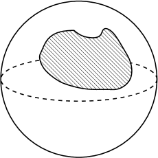
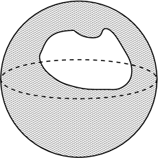
Figure 1: The action corresponds to the area bounded by the image of spacetime. Two different bounding surfaces are pictured.

The WZW action is defined by mapping two-dimensional spacetime, identified with $S^{2}$, into $S^{3}$ (i.e., $x\to\Phi(x)$), and then integrating $\omega$ over a three-dimensional manifold $M^{3}$ with spacetime as its boundary, as in Fig. 1. Consistency requires that different bounding manifolds give equivalent actions, up to a multiple of $2\pi$, so that observables derived from $e^{i\Gamma_{0}}$ are unambiguous. Since $\pi_{3}(S^{3})=\mbox{\boldmath$Z$\unboldmath}$, inequivalent mappings are labeled by an integer winding number. Using that the volume of $S^{3}$ is $2\pi^{2}$, the properly normalized action is

$$\Gamma_{0}(\Phi)=p\times 2\pi\times{1\over 2\pi^{2}}\int_{M^{3}}\omega={p\over\pi}\int_{M^{3}}\omega\,,$$ (5)

where $p$ is an integer. While the action (5) is not expressed in a form that is manifestly both two-dimensional and globally $SU(2)\times U(1)$ invariant its construction ensures that it has both properties. With the quantization condition in place, the action is manifestly local in the sense that small changes in $\Phi(x)$ result in small changes in the action (modulo $2\pi$).

II.2 Gauging the topological action

Let us proceed to perform a “brute force” gauging of the action. Consider the local variation:

$$\Phi\to e^{i(\epsilon+\epsilon_{0})}\Phi\,,$$ (6)

where $\epsilon=\sum_{A=1}^{3}\epsilon^{A}\sigma^{A}$ and $\epsilon_{0}$ generate $SU(2)$ and $U(1)$ transformations respectively. The corresponding variation of $\Gamma_{0}$ is

$$\delta\Gamma_{0} ={ip\over 2\pi}\int_{M^{3}}d\epsilon_{0}d\Phi^{\dagger}d\Phi+\Phi^{\dagger}d\epsilon\Phi d\Phi^{\dagger}d\Phi-\Phi^{\dagger}d\Phi\Phi^{\dagger}d\epsilon d\Phi$$

$$\qquad+\Phi^{\dagger}d\Phi d\Phi^{\dagger}d\epsilon\Phi$$

$$={ip\over 2\pi}\int_{M^{3}}d\big{[}\epsilon_{0}d\Phi^{\dagger}d\Phi+\Phi^{\dagger}\epsilon\Phi d\Phi^{\dagger}d\Phi+\Phi^{\dagger}d\Phi\Phi^{\dagger}\epsilon d\Phi$$

$$\qquad+\Phi^{\dagger}d\Phi d\Phi^{\dagger}\epsilon\Phi\big{]}$$

$$\qquad-2\epsilon^{A}\left[d\Phi^{\dagger}d\Phi(\Phi^{\dagger}\sigma^{A}d\Phi+d\Phi^{\dagger}\sigma^{A}\Phi)\right]\,.$$ (7)

It is not obvious from this expression that the variation is four-dimensional. However, using the identity

$$d(\Phi^{\dagger}\sigma^{A}\Phi)d\Phi^{\dagger}d\Phi=0\,,$$ (8)

which holds when $\Phi^{\dagger}\Phi=1$, it follows using Stokes theorem in (II.2) that

$$\delta\Gamma_{0}={ip\over 2\pi}\int_{M^{2}}\epsilon_{0}d\Phi^{\dagger}d\Phi+\Phi^{\dagger}\epsilon\Phi d\Phi^{\dagger}d\Phi+\Phi^{\dagger}d\Phi\Phi^{\dagger}\epsilon d\Phi\\ +\Phi^{\dagger}d\Phi d\Phi^{\dagger}\epsilon\Phi\,.$$ (9)

It is now not obvious that the variation is purely local, i.e., that it vanishes when $d\epsilon=0$, $d\epsilon_{0}=0$. However, if we further make use of the identity,

$$d\Phi^{\dagger}\sigma^{A}d\Phi=d(\Phi^{\dagger}\sigma^{A}\Phi)\Phi^{\dagger}d\Phi-\Phi^{\dagger}\sigma^{A}\Phi d\Phi^{\dagger}d\Phi\,,$$ (10)

then, after an integration by parts, (9) is equivalent to

$$\delta\Gamma_{0}={ip\over 4\pi}\int_{M^{2}}-2d\epsilon_{0}\Phi^{\dagger}d\Phi+\Phi^{\dagger}d\epsilon d\Phi+d\Phi^{\dagger}d\epsilon\Phi\,.$$ (11)

The identities (8) and (10) can be checked explicitly, and can be understood in terms of spherical geometry, as described in Appendix A.

From (11) we see that the local variation can be compensated by adding a term with one gauge field,

$$\Gamma_{1}={ip\over 4\pi}\int_{M^{2}}2A_{0}\Phi^{\dagger}d\Phi-\Phi^{\dagger}Ad\Phi-d\Phi^{\dagger}A\Phi\,,$$ (12)

where $A_{0}$ and $A=\sum_{B=1}^{3}A^{B}\sigma^{B}$ transform as

$$\delta A_{0}=d\epsilon_{0}\,,\quad\delta A=d\epsilon+i[\epsilon,A]\,.$$ (13)

The residual variation is

$$\delta(\Gamma_{0}+\Gamma_{1}) ={p\over 2\pi}\int_{M^{2}}\frac{1}{2}{\rm Tr}(Ad\epsilon)-A_{0}d\epsilon_{0}-A_{0}\Phi^{\dagger}d\epsilon\Phi$$

$$\qquad-d\epsilon_{0}\Phi^{\dagger}A\Phi\,.$$ (14)

Finally, adding a term with two gauge fields,

$$\Gamma_{2}={p\over 2\pi}\int_{M^{2}}A_{0}\Phi^{\dagger}A\Phi\,,$$ (15)

removes all $\Phi$ dependent terms in the variation of $\Gamma_{0}+\Gamma_{1}$. The fully gauged action is

$$\Gamma_{WZW} =\Gamma_{0}+\Gamma_{1}+\Gamma_{2}$$

$$=\Gamma_{0}+{ip\over 4\pi}\int_{M^{2}}-\Phi^{\dagger}Ad\Phi-d\Phi^{\dagger}A\Phi+2A_{0}\Phi^{\dagger}d\Phi$$

$$\qquad-2iA_{0}\Phi^{\dagger}A\Phi\,,$$ (16)

with $\Gamma_{0}$ as in (5). In fact, the compensating terms (12) and (15) are not unique. An additional gauge-invariant operator can appear, whose coefficient is not quantized:

$$\Gamma_{G.I.}={p\over\pi}\int_{M^{2}}c\Phi^{\dagger}(dA-iA^{2})\Phi\,.$$ (17)

To gain some intuition on the physical content of this action, we can consider the coordinates

$$\Phi=\exp\left[i\left(\begin{array}[]{cc}0&h_{1}-ih_{2}\\ h_{1}+ih_{2}&2\eta\end{array}\right)\right]\left(\begin{array}[]{c}0\\ 1\end{array}\right)\,.$$ (18)

The action is then (displaying the first nonvanishing term from $\Gamma_{0}$ in addition to nonzero terms involving gauge fields through second order in mesons),

$$\Gamma_{WZW} ={p\over\pi}\int_{M^{2}}-i\eta dh^{+}dh^{-}+\dots$$

$$-Bd\eta+{i\over 4}D(h^{-}dh^{+}-h^{+}dh^{-})$$

$$+\frac{1}{4}(1+i\eta)C^{+}dh^{-}+\frac{1}{4}(1-i\eta)C^{-}dh^{+}$$

$$-{3i\over 4}(C^{+}h^{-}-C^{-}h^{+})d\eta$$

$$-{i\over 4}(B+D)\left[(1+i\eta)C^{+}h^{-}-(1-i\eta)C^{-}h^{+}\right]$$

$$+\frac{1}{4}BD\left(1-2h^{+}h^{-}\right)+\dots\,.$$ (19)

Here $h^{\pm}=h_{1}\mp ih_{2}$, and the gauge bosons are separated in terms of the light “photon” $B$, and the heavy $D$ and $C^{\pm}$:

$$A+A_{0}\equiv\left(\begin{array}[]{cc}B&C^{+}\\ C^{-}&D\end{array}\right)\,.$$ (20)

The gauge invariant operator (17) is

$$\Gamma_{G.I.} =c\int_{M^{2}}ih^{+}(1-i\eta)[dC^{-}-iC^{-}(B-D)]$$

$$\qquad-ih^{-}(1+i\eta)[dC^{+}+iC^{+}(B-D)]$$

$$\qquad-(1-2h^{-}h^{+})\left[\frac{1}{2}(dB-dD)-iC^{+}C^{-}\right]\,.$$ (21)

II.3 Anomaly

The action (II.2) has the anomalous gauge variation,

$$\delta\Gamma_{WZW}={p\over 4\pi}\int_{M^{2}}{\rm Tr}(\epsilon dA)-2\epsilon_{0}dA_{0}\,.$$ (22)

This can be viewed as the anomaly for a doublet of left-handed fermions and a single right-handed fermion transforming under $SU(2)\times U(1)$ as

$$\Psi_{L}\to e^{i(\epsilon\mp\epsilon_{0})}\Psi_{L}\,,\quad q_{R}\to e^{\mp 2i\epsilon_{0}}q_{R}\,.$$ (23)

II.4 Equivalence to $SU(2)_{L}\times SU(2)_{R}/SU(2)_{V}$

We will discuss later an equivalence between the $SU(3)/SU(2)$ WZW term and a limit of the $SU(3)_{L}\times SU(3)_{R}/SU(3)_{V}$ WZW term. In the present example, since $SU(2)_{L}\times SU(2)_{R}/SU(2)_{V}\cong SU(2)\cong S^{3}$, a similar but simpler equivalence holds.

Let us for the moment ignore the $U(1)$ factor in $SU(2)\times U(1)$. The two-dimensional action for $SU(2)_{L}\times SU(2)_{R}/SU(2)_{V}$ is the gauged version of 

$$\Gamma_{0}=-{p\over 12\pi}\int_{M^{3}}{\rm Tr}(\beta^{3})\,,$$ (24)

where we write

$$\alpha=dU\,U^{\dagger}\,,\quad\beta=U^{\dagger}dU\,.$$ (25)

Performing a local gauge variation of the action (24), and compensating with gauge fields, the gauged action becomes

$$\Gamma_{WZW}=\Gamma_{0}+{p\over 4\pi}\int_{M^{2}}{\rm Tr}\left[-iA_{L}\alpha-iA_{R}\beta+A_{L}UA_{R}U^{\dagger}\right]\,.$$ (26)

The anomalous gauge variation of the action is

$$\delta\Gamma_{WZW}={p\over 4\pi}\int_{M^{2}}{\rm Tr}\left(\epsilon_{L}dA_{L}-\epsilon_{R}dA_{R}\right)\,.$$ (27)

We can implement the diffeomorphism between $SU(2)$ and $S^{3}$ by

$$\Phi(x)=U(x)\left(\begin{array}[]{c}0\\ 1\end{array}\right)\,.$$ (28)

Let us also identify,

$$A_{L}=A\,,\quad A_{R}=0\,.$$ (29)

The actions (II.2), taken at $A_{0}=0$, and (26), are now easily shown to be identical. First note that the variations (22) and (27) coincide, so that the actions differ only by gauge invariant operators. The equivalence is established using the $SU(2)$ identities, for arbitrary $SU(2)$-valued one-forms $\alpha$, $\beta$, and for an arbitrary one-dimensional projector $P^{2}=P$:

$${\rm Tr}(P\alpha P\alpha^{2}) =\frac{1}{6}{\rm Tr}(\alpha^{3})\,,$$

$${\rm Tr}[P(\alpha\beta-\beta\alpha)] ={\rm Tr}(\alpha\beta)\,.$$ (30)

In particular, with

$$P=\left(\begin{array}[]{cc}0&0\\ 0&1\end{array}\right)\,,$$ (31)

and with $\Phi$ and $U$ as in (28), it follows that

$${-p\over 12\pi}{\rm Tr}(\alpha^{3}) ={p\over 2\pi}\Phi^{\dagger}d\Phi d\Phi^{\dagger}d\Phi\,,$$

$${-ip\over 4\pi}{\rm Tr}(A\alpha) ={-ip\over 4\pi}(\Phi^{\dagger}Ad\Phi+d\Phi^{\dagger}A\Phi)\,,$$ (32)

establishing the equivalence between the actions (II.2) and (26), with $c=0$ in (17). The equivalence can be extended to include the $U(1)$ factor by writing

$$A_{L}=A-A_{0}\,,\quad A_{R}=-2A_{0}P\,,$$ (33)

with $P$ as in (31).

II.5 Counterterms and anomaly integration

The gauged WZW term for $SU(2)\times U(1)/U(1)$ in two dimensions affords a simple context to see the equivalence between “top down” anomaly integration and the preceding “bottom up” approach. Here we find the necessary counterterm for the integration to be possible.

Let us choose the orientation of $\Phi$ which breaks the global $SU(2)\times U(1)$ symmetry as

$$\langle\Phi\rangle=\left(\begin{array}[]{c}0\\ 1\end{array}\right)\,.$$ (34)

The components of the $SU(2)\times U(1)$ gauge bosons are defined as in (20), and for the corresponding gauge transformations in (6) we write:

$$\epsilon+\epsilon_{0}\equiv\left(\begin{array}[]{cc}\epsilon_{B}&\epsilon_{C^{+}}\\ \epsilon_{C^{-}}&\epsilon_{D}\end{array}\right)\,.$$ (35)

The anomaly expression (22) then becomes

$$\delta\Gamma_{WZW}={p\over 4\pi}\int_{M^{2}}d\epsilon_{B}D+d\epsilon_{D}B-d\epsilon_{C^{+}}C^{-}-d\epsilon_{C^{-}}C^{+}\,.$$ (36)

We notice that $\delta\Gamma_{WZW}$ vanishes when both the gauge variation and the background gauge fields are restricted to the unbroken $U(1)$ subgroup—i.e., $\epsilon_{C^{\pm}}=\epsilon_{D}=0$ and $C^{\pm}=D=0$. However, in the presence of arbitrary $C^{\pm}$ and $D$ fields, the action still has an anomalous gauge variation even when $\epsilon_{C^{\pm}}=\epsilon_{D}=0$. We can find a counterterm that preserves gauge invariance in the unbroken fields for arbitrary background fields, and converts the anomaly to the “covariant” form. This is the analog of the Bardeen counterterm Bardeen:1969md ; Bardeen:1984pm , which for the present case is

$$\Gamma_{c}(A,A_{0})=-\Gamma_{WZW}(A,A_{0},\Phi=\langle\Phi\rangle)\,,$$ (37)

where $\langle\Phi\rangle$ is the orientation of $\Phi$ which breaks the global symmetry. Taking $\langle\Phi\rangle$ as in (34), and using (II.2), the counterterm is 

$$\Gamma_{c}=-{p\over 4\pi}\int_{M^{2}}BD\,.$$ (38)

With the addition of the counterterm, the gauge variation becomes

$$\delta(\Gamma_{WZW}+\Gamma_{c}) ={p\over 4\pi}\int_{M^{2}}-2\epsilon_{D}dB+\epsilon_{C^{+}}dC^{-}+\epsilon_{C^{-}}dC^{+}$$

$$\qquad-i\left(\epsilon_{C^{+}}C^{-}-\epsilon_{C^{-}}C^{+}\right)(B+D)\,,$$ (39)

and we see that the resulting action is gauge invariant under the unbroken subgroup, in the presence of arbitrary background gauge fields.

For a general orientation of $\langle\Phi\rangle$, the variation of the complete action with counterterm is

$$\delta(\Gamma_{WZW}+\Gamma_{c}) ={p\over 4\pi}\int_{M^{2}}{\rm Tr}\bigg{[}$$

$$\qquad\epsilon\left(dA-2PdA_{0}+2i[A,P]A_{0}\right)$$

$$\qquad+\epsilon_{0}\left(-dA_{0}+2dAP\right)\bigg{]}$$

$$\equiv\int_{M^{2}}\epsilon^{a}{\cal A}^{a}[A]\,,$$ (40)

where in the last line ${\cal A}$ denotes the (covariant) anomaly, and the sum runs over broken generators.

We remark in passing that since the action is well-defined, by its topological construction, the gauge variation (22) is guaranteed to be a “consistent” anomaly. That is,

$$\Delta^{a}(x){\cal A}^{b}[A(y)]-\Delta^{b}(y){\cal A}^{a}[A(x)]=f^{abc}{\cal A}^{c}[A(x)]\delta(x-y)\,,$$ (41)

where $f^{abc}$ are the structure constants of $SU(2)\times U(1)$, and $\Delta^{a}$ are generators of gauge transformations on the gauge fields:

$$\Delta^{a}=-\partial_{\mu}{\delta\over\delta A_{\mu}^{a}}-f^{abc}A^{b}_{\mu}{\delta\over\delta A^{c}_{\mu}}\,.$$ (42)

Adding the Bardeen counterterm does not change the consistency of the anomaly, since it is again a well-defined object (the reduction of the topological action to a constant value for the meson field). Eq.(41) can be verified to hold using the explicit form of the anomaly in (II.5).

Given a consistent anomaly that vanishes on the unbroken subgroup ($U(1)$ in this case), it is possible to “integrate” the anomaly to obtain an effective action with the stated anomalous gauge variation. The solution is Wess:1971yu :

$$\Gamma_{WZW}+\Gamma_{c}=\int_{M^{2}}\int_{0}^{1}dt\,\pi^{a}{\cal A}^{a}[A^{t}]\,.$$ (43)

Under a gauge transformation $e^{i(\epsilon+\epsilon_{0})}\in SU(2)\times U(1)$, the generalized pions transform as a nonlinear realization Coleman:1969sm

$$e^{i\pi}\to e^{i(\epsilon+\epsilon_{0})}e^{i\pi}e^{-i\epsilon^{\prime}(\epsilon+\epsilon_{0},\pi)}\,.$$ (44)

The quantity $A^{t}$ in (43) is a gauge-transformed field depending on pions:

$$A^{t}=e^{-it\pi}(A+id)e^{it\pi}\,.$$ (45)

Here $\epsilon^{\prime}$ is an element of the unbroken group chosen such that $e^{i\pi}$ is generated by the broken subgroup. This defines a unique local transformation $\pi\to\pi^{\prime}$. It is readily verified using (44) and (45) that (43) is a solution to (II.5).

With the coordinates for the pions as in (18), i.e. $\Phi=e^{i\pi}(0,1)^{T}$, and the gauge fields as in (20), we have

$$A^{t}=\left(\begin{array}[]{cc}B&C^{+}\\ C^{-}&D\end{array}\right)+it\left(\begin{array}[]{cc}h^{-}C^{+}-h^{+}C^{-}&(B-D)h^{+}+2\eta C^{+}+idh^{+}\\ (D-B)h^{-}-2\eta C^{-}+idh^{-}&h^{+}C^{-}-h^{-}C^{+}+2id\eta\end{array}\right)+\dots\,.$$ (46)

Substituting these explicit expression into (43) yields the result in (II.2), minus the term with zero pions that has been subtracted by the counterterm. In order to avoid discontinuous jumps in the action under small fluctuations in the pion fields, the action should be quantized as in (5).

III $SU(3)\times U(1)/SU(2)\times U(1)$ in four dimensions

Although algebraically more complicated, the case of $SU(3)\times U(1)/SU(2)\times U(1)$ in four dimensions proceeds in complete analogy to the above case of $SU(2)\times U(1)/U(1)$ in two dimensions.

III.1 Topological action and quantization condition

The field space is described by the three-component complex scalar field,

$$\Phi(x)=\left(\begin{array}[]{c}\phi^{1}(x)+i\phi^{2}(x)\\ \phi^{3}(x)+i\phi^{4}(x)\\ \phi^{5}(x)+i\phi^{6}(x)\end{array}\right)\,,$$ (47)

satisfying

$$\Phi^{\dagger}\Phi=\sum_{i=1}^{6}(\phi^{i})^{2}=1\,.$$ (48)

The starting point for the topological construction is a closed five-form that is invariant under global $SU(3)\times U(1)$ transformations. The unique choice is

$$\omega=-{i\over 8}\Phi^{\dagger}d\Phi d\Phi^{\dagger}d\Phi d\Phi^{\dagger}d\Phi\,,$$ (49)

where the normalization is chosen such that $\omega$ is the volume element on the five-sphere. Noting that $\pi_{4}(S^{5})=0$ and $\pi_{5}(S^{5})=\mbox{\boldmath$Z$\unboldmath}$, and using that the volume of the five sphere is $\pi^{3}$, the WZW action is well-defined up to multiples of $2\pi$ if we take

$$\Gamma_{0}(\Phi)={2p\over\pi^{2}}\int_{M^{5}}\omega\,,$$ (50)

where $M^{5}$ is a five-dimensional manifold with spacetime $M^{4}$ as its boundary, and $p$ is an arbitrary integer.

III.2 Gauging the topological action

We consider again the local variation

$$\Phi\to e^{i(\epsilon+\epsilon_{0})}\Phi\,,$$ (51)

where $\epsilon=\sum_{A=1}^{8}\epsilon^{A}\lambda^{A}$ and $\epsilon_{0}$ generate $SU(3)$ and $U(1)$ transformations respectively. The corresponding variation of $\Gamma_{0}$ is

$$\delta\Gamma_{0} ={p\over 4\pi^{2}}\int_{M^{5}}d\bigg{[}\epsilon_{0}(d\Phi^{\dagger}d\Phi)^{2}+\Phi^{\dagger}\epsilon\Phi(d\Phi^{\dagger}d\Phi)^{2}-2(\Phi^{\dagger}\epsilon d\Phi+d\Phi^{\dagger}\epsilon\Phi)\Phi^{\dagger}d\Phi d\Phi^{\dagger}d\Phi\bigg{]}-3\epsilon^{A}d(\Phi^{\dagger}\lambda^{A}\Phi)(d\Phi^{\dagger}d\Phi)^{2}\,.$$ (52)

To see that the result is four-dimensional, we notice that

$$d(\Phi^{\dagger}\lambda^{A}\Phi)(d\Phi^{\dagger}d\Phi)^{2}=0\,,$$ (53)

for fields confined to the five-sphere. The gauge variation then becomes

$$\delta\Gamma_{0} ={p\over 4\pi^{2}}\int_{M^{4}}\epsilon_{0}(d\Phi^{\dagger}d\Phi)^{2}+\epsilon^{A}\bigg{[}\Phi^{\dagger}\lambda^{A}\Phi(d\Phi^{\dagger}d\Phi)^{2}$$

$$\qquad+2\Phi^{\dagger}d\Phi d(\Phi^{\dagger}\lambda^{A}\Phi)d\Phi^{\dagger}d\Phi\bigg{]}\,.$$ (54)

By construction, the gauge variation must vanish for constant $\epsilon_{0}$ and $\epsilon$. To see this explicitly, we notice that for $\Phi^{\dagger}\Phi=1$ we have the $SU(3)$ identities

$$\Phi^{\dagger}\lambda^{A}\Phi(d\Phi^{\dagger}d\Phi)^{2}+2\Phi^{\dagger}d\Phi d(\Phi^{\dagger}\lambda^{A}\Phi)d\Phi^{\dagger}d\Phi=\\ -2d\Phi^{\dagger}\lambda^{A}d\Phi d\Phi^{\dagger}d\Phi\,,$$ (55)

so that finally

$$\delta\Gamma_{0}={p\over 4\pi^{2}}\int_{M^{4}}\left(\Phi^{\dagger}d\epsilon d\Phi+d\Phi^{\dagger}d\epsilon\Phi-d\epsilon_{0}\Phi^{\dagger}d\Phi\right)d\Phi^{\dagger}d\Phi\,.$$ (56)

This variation can be cancelled by a term with one gauge field, and so on. Details of the derivation in this case are presented in Appendix A. The complete result reads

$$\Gamma_{WZW}(\Phi,A,A_{0}) =\Gamma_{0}(\Phi)+{p\over 4\pi^{2}}\int_{M^{4}}\sum_{i=1}^{4}{\cal L}_{i}+{\cal L}_{G.I.}\,,$$ (57)

where terms with 1,2,3,4 gauge fields are:

$${\cal L}_{1} =A_{0}\Phi^{\dagger}d\Phi d\Phi^{\dagger}d\Phi-\left(\Phi^{\dagger}Ad\Phi+d\Phi^{\dagger}A\Phi\right)d\Phi^{\dagger}d\Phi\,,$$

$${\cal L}_{2} =iA_{0}dA_{0}\Phi^{\dagger}d\Phi-idA_{0}\Phi^{\dagger}A\Phi\Phi^{\dagger}d\Phi-2iA_{0}\Phi^{\dagger}A\Phi d\Phi^{\dagger}d\Phi+{i\over 2}\left[(d\Phi^{\dagger}A\Phi)^{2}-(\Phi^{\dagger}Ad\Phi)^{2}\right]$$

$$\qquad+{i\over 4}\left[\Phi^{\dagger}(AdA+dAA)d\Phi+d\Phi^{\dagger}(AdA+dAA)\Phi\right]-{i\over 2}\Phi^{\dagger}(AdA+dAA)\Phi\Phi^{\dagger}d\Phi-{i\over 2}{\rm Tr}(AdA)\Phi^{\dagger}d\Phi$$

$$\qquad+{i\over 4}\left[\Phi^{\dagger}dA\Phi(d\Phi^{\dagger}A\Phi+\Phi^{\dagger}Ad\Phi)+\Phi^{\dagger}A\Phi(\Phi^{\dagger}dAd\Phi-d\Phi^{\dagger}dA\Phi)\right]\,,$$

$${\cal L}_{3} =A_{0}dA_{0}\Phi^{\dagger}A\Phi+A_{0}\left[-\Phi^{\dagger}A\Phi d(\Phi^{\dagger}A\Phi)+\frac{1}{3}{\rm Tr}(AdA)\right]-\frac{1}{6}\Phi^{\dagger}A^{2}\Phi(\Phi^{\dagger}Ad\Phi+d\Phi^{\dagger}A\Phi)$$

$$\qquad+\frac{1}{6}\Phi^{\dagger}A\Phi(\Phi^{\dagger}A^{2}d\Phi-d\Phi^{\dagger}A^{2}\Phi)+\frac{1}{6}\Phi^{\dagger}(dAA^{2}-A^{2}dA)\Phi+\frac{1}{3}(\Phi^{\dagger}A^{3}d\Phi+d\Phi^{\dagger}A^{3}\Phi)-\frac{2}{3}\Phi^{\dagger}A^{3}\Phi\Phi^{\dagger}d\Phi$$

$$\qquad-\frac{1}{3}{\rm Tr}(A^{3})\Phi^{\dagger}d\Phi-\frac{1}{2}\Phi^{\dagger}(AdA+dAA)\Phi\Phi^{\dagger}A\Phi-\frac{1}{3}{\rm Tr}(AdA)\Phi^{\dagger}A\Phi\,,$$

$${\cal L}_{4} =-{i\over 4}A_{0}{\rm Tr}(A^{3})-{3i\over 4}\Phi^{\dagger}A\Phi\Phi^{\dagger}A^{3}\Phi-{i\over 4}\Phi^{\dagger}A\Phi{\rm Tr}(A^{3})\,.$$ (58)

There are additional four-form operators that are separately gauge-invariant:

$${\cal L}_{G.I.}=c_{1}\,\left[\Phi^{\dagger}(dA-iA^{2})\Phi\right]^{2}$$

$$\quad+c_{2}\,i\Phi^{\dagger}(dA-iA^{2})\Phi D\Phi^{\dagger}D\Phi$$

$$\quad+c_{3}\,\Phi^{\dagger}(dA-iA^{2})^{2}\Phi$$

$$\quad+c_{4}\,\Phi^{\dagger}D\Phi\left[\Phi^{\dagger}(dA-iA^{2})D\Phi-(D\Phi^{\dagger})(dA-iA^{2})\Phi\right]\,,$$

$$\quad+c_{5}\,dA_{0}\Phi^{\dagger}(dA-iA^{2})\Phi\,,$$ (59)

where the covariant derivative acts as

$$D\Phi=d\Phi-i(A+A_{0})\Phi\,.$$ (60)

III.3 Anomaly

The gauge variation of the action (57) is independent of $\Phi$,

$$\delta\Gamma =-{p\over 12\pi^{2}}\int_{M^{4}}{\rm Tr}\bigg{\{}\epsilon\left[(dA)^{2}-{i\over 2}d(A^{3})\right]-\frac{1}{2}\epsilon_{0}\left[(dA)^{2}-{i\over 2}d(A^{3})\right]-\frac{1}{2}\epsilon\left[2dA\,dA_{0}-{i\over 2}d(A_{0}A^{2})\right]\bigg{\}}+3\epsilon_{0}(dA_{0})^{2}$$

$$=-{2p\over 24\pi^{2}}\int_{M^{4}}{\rm Tr}\bigg{\{}\left(\epsilon-\frac{1}{2}\epsilon_{0}\openone_{3}\right)\left[\left(dA-{1\over 2}dA_{0}\openone_{3}\right)^{2}-{i\over 2}d\left[\left(A-\frac{1}{2}A_{0}\openone_{3}\right)^{3}\right]\right]\bigg{\}}-\left(-\frac{3}{2}\epsilon_{0}\right)\left(-\frac{3}{2}dA_{0}\right)^{2}\,.$$

Note that this is the anomaly for a triplet of left-handed fermions $\Psi_{L}=(\psi_{L}^{1},\psi_{L}^{2},\psi_{L}^{3})^{T}$, and a single right-handed fermion, $\psi_{R}$, each with $2p$ internal coordinates (“colors”), transforming under $SU(3)\times U(1)$ as

$$\Psi_{L}\to e^{i\left(\epsilon-\frac{1}{2}\epsilon_{0}\right)}\Psi_{L}\,,\qquad\psi_{R}\to e^{-{3i\over 2}\epsilon_{0}}\,.$$ (62)

III.4 Equivalence to $SU(3)\times SU(3)/SU(3)$

In a manner similar to the two-dimensional example, we can find an equivalence of the $SU(3)/SU(2)$ WZW term to a limit of the $SU(3)\times SU(3)/SU(3)$ WZW term. Recall that the latter in its ungauged form may be written

$$\Gamma_{SU(3)\times SU(3)/SU(3)}=-{iN\over 240\pi^{2}}\int_{M^{5}}{\rm Tr}(\beta^{5})\,,$$ (63)

with $\beta$ as in (25).

We start from the nonlinear realization of $SU(3)$ on $SU(3)/SU(2)$:

$$\xi\to e^{i\epsilon}\xi e^{-i\epsilon^{\prime}(\epsilon,\xi)}\,,$$ (64)

where $\xi$ is an $SU(3)$ matrix given by the exponential of broken generators. The equivalence is stated as

$$\Gamma_{SU(3)/SU(2)}(p,\Phi,A)=\\ \Gamma_{SU(3)\times SU(3)/SU(3)}(2p,\tilde{U},\tilde{A}_{L},\tilde{A}_{R})\,.$$ (65)

The dictionary is

$$\tilde{U} =\xi\,,$$

$$\tilde{A}_{L} =A\,,$$

$$\tilde{A}_{R} =\sum_{A=1}^{3}{\lambda_{A}\over 2}{\rm Tr}(\lambda_{A}[\xi^{\dagger}(A+id)\xi])\,,$$ (66)

where $SU(3)/SU(2)\cong S^{5}$ is implemented by

$$\Phi=\xi\left(\begin{array}[]{c}0\\ 0\\ 1\end{array}\right)\,.$$ (67)

Note that $\tilde{A}_{R}$ is the projection of $\xi^{\dagger}(A+id)\xi$ onto the unbroken $SU(2)$ subgroup.

Equation (III.3) shows that the actions (65) have the same gauge variation, i.e., the actions are equivalent up to gauge invariant operators. The exact equivalence can again be demonstrated explicitly. For example, introducing

$$\beta=\xi^{\dagger}d\xi\,,$$ (68)

the equivalence for terms without gauge fields follows from the form identity

$${-2i\over 240\pi^{2}}{\rm Tr}\bigg{[}\beta^{5}$$

$$\quad+5d\left(-\hat{\beta}\beta^{3}+\frac{1}{2}(\hat{\beta}\beta)^{2}+(d\hat{\beta}\hat{\beta}+\hat{\beta}d\hat{\beta})\beta+\hat{\beta}^{3}\beta\right)\bigg{]}$$

$$={-i\over 4\pi^{2}}\Phi^{\dagger}d\Phi(d\Phi^{\dagger}d\Phi)^{2}\,,$$ (69)

using (50) and the gauged version of (63). Here $\hat{\beta}$ is the projection of $\beta$ onto the unbroken $SU(2)$ subgroup, as in (III.4).

The coefficients of gauge invariant operators can be fixed by examining the equivalence at $U=\xi=\openone_{3}$. This yields

$$c_{1} =c_{2}=c_{3}=0\,,\quad c_{4}={7\over 12}\,.$$ (70)

The equivalence can be extended to $SU(3)\times U(1)/SU(2)\times U(1)$ by setting

$$A_{L}=\tilde{A}_{L}-\frac{1}{2}A_{0}\,,\quad A_{R}=\tilde{A}_{R}-\frac{3}{2}A_{0}\left(\begin{array}[]{ccc}0\\ &0\\ &&1\end{array}\right)\,,$$ (71)

and

$$c_{5}=0\,.$$ (72)

A physical basis for the equivalence is the “eating and decoupling” scenario discussed in Hill:2007nz . Here $\xi$ is extended to a full unitary matrix $U\in SU(3)_{L}\times SU(3)_{R}/SU(3)_{V}$, with $SU(3)$ made to act on the left. If we couple $SU(2)$ gauge fields to the unbroken right-handed symmetries, then the extraneous NGB’s are eaten by these fields. In a strong coupling limit, the extra gauge fields become nondynamical, enforcing the locking condition (III.4). Since $SU(2)$ does not have a continuous anomaly, the gauging is anomaly free provided that the coefficient, $N$, of the WZW term is even.

III.5 (No) Skyrmion

In the previous section, it was shown that the WZW term for $SU(3)/SU(2)$ is equivalent to a certain limit of $SU(3)\times SU(3)/SU(3)$, but with an even number of colors. We thus expect that the Skyrmion solution in the latter case is absent. This is verified by noticing that $\pi_{3}(S^{5})=0$. This can also be seen from the fact that no analog of a conserved Goldstone-Wilczek baryon current Goldstone:1981kk can be constructed from $\Phi$, since

$$(\Phi^{\dagger}d\Phi)^{3}=0\,,$$ (73)

and

$$d[\Phi^{\dagger}d\Phi d\Phi^{\dagger}d\Phi]=(d\Phi^{\dagger}d\Phi)^{2}\neq 0\,.$$ (74)

IV Summary

Much of the complexity of WZW terms stems from the difficulty in identifying a five-sphere inside a nontrivial field space such as $SU(3)$. In the case of $SU(3)/SU(2)$, the field space is the five-sphere, giving rise to a particularly simple WZW term. The present paper gives explicit results for the fully gauged action.

The action (57) plays a role in phenomenological models of extended Higgs sectors of electroweak symmetry breaking. For example, the $SU(3)/SU(2)$ Little Higgs model Schmaltz:2004de with generation-independent gauging requires a WZW term for anomaly cancellation. A variant with distinct third-generation quantum numbers Frampton:1992wt also allows a WZW term, and the quantization of the action (50) restricts possible strongly-coupled UV completions to those with even numbers of “colors”. The WZW term in general gives rise to interactions violating a discrete “T parity” Cheng:2003ju ; Cheng:2004yc . Related applications have been discussed in Hill:2007nz ; Hill:2007zv ; Hill:2007eh ; Freitas:2008mq ; Krohn:2008ye ; Csaki:2008se ; Lane:2009ct . The same WZW term would appear in extensions that incorporate a custodial symmetry by embedding $SU(3)$ into larger spaces, e.g. $SU(4)/Sp(4)$ or $SO(6)/SO(5)$ in place of $SU(3)/SU(2)$ Bai:2008cf ; Batra:2008jy .

Another application is to the description of “decoupled” fermions in the Standard Model, and the associated WZW term built from the Higgs field D'Hoker:1984ph . Naively, since the NGB’s of the Higgs field live on $SU(2)\times U(1)/U(1)\cong S^{3}$, and $\pi_{5}(S^{3})=0$, there is no associated topological interaction. This is reminiscent of the fact that a topological derivation of the $U(2)_{L}\times U(2)_{R}/U(2)_{V}$ WZW term requires embedding inside a larger $U(n)$ space, $n\geq 3$. A similar reduction of $SU(3)\times U(1)/SU(2)\times U(1)$ gives a topological derivation of the WZW term for the Standard Model Higgs. In particular, taking

$$\Phi=\left(\begin{array}[]{c}0\\ H\end{array}\right),\quad A=\left(\begin{array}[]{cc}0\\ &W\end{array}\right),\quad A_{0}=\frac{1}{2}B\,,$$ (75)

with $W=W^{A}\sigma^{A}/2$ and $H$ an isodoublet Higgs field, (57) yields the anomalous interaction that would describe, e.g., the result of integrating out a generation of heavy leptons, or heavy quarks, after spontaneous symmetry breaking. Consider fermion doublets $\Psi_{L}$ and $\Psi_{R}$ coupled to $SU(2)_{L}\times U(1)_{Y}$ gauge fields

$$A_{L}=W+yB\,,\quad A_{R}=\left(y+{\sigma^{3}\over 2}\right)B\,.$$ (76)

The anomalous variation of the gauged fermion action is

$$\delta\Gamma=-{y\over 24\pi^{2}}\int_{M^{4}}{\rm Tr}\bigg{\{}\epsilon_{W}\left[2dWdB-{i\over 2}d(BW^{2})\right]\\ +\epsilon_{B}\left[(dW)^{2}-{i\over 2}d(W^{3})\right]\bigg{\}}-{3\over 2}\epsilon_{B}(dB)^{2}\,.$$ (77)

Using (75) in (III.3) shows that the anomaly of the reduced WZW term matches that of the fermions provided

$$p=-2y\,.$$ (78)

In particular, integer values of $p$ are sufficient to describe a single generation of quarks or leptons. The custodial symmetry limit considered in D'Hoker:1984ph is recovered for particular values of the coefficients in (III.2). These can be fixed by considering e.g. the action at $H=(0,1)^{T}$, and are

$$c_{1}-\frac{1}{2}c_{2}=c_{3}=c_{5}=0\,,\quad c_{4}=\frac{1}{2}\,.$$ (79)

The operator corresponding to the remaining linear combination vanishes in this case due to relations such as (8),(10).

Acknowledgements.

The author thanks C. Hill for many insightful discussions stemming from Refs. Hill:2007nz ; Hill:2007zv , which motivated this work. This work was supported by NSF Grant No. 0855039.

Appendix A Differential geometry identities

The brute force gauging of the $SU(3)/SU(2)$ WZW term involves the use of several nontrivial identities, such as (55), relating combinations of the Gell-Mann matrices and complex triplets with $\Phi^{\dagger}\Phi=1$. Similar identities, (8) and (10), occur in the two-dimensional example. While not essential at the practical level, it is helpful to use the language of differential geometry in order to see the origin of these manipulations. For more details, see Ref. Hull:1990ms , whose notations are largely adopted here.

A.1 $SU(2)\times U(1)$ in two dimensions

To introduce notation, consider $SU(2)\times U(1)/U(1)$ in two dimensions. As discussed above (1), we may identify $\Phi=(\phi^{1}(x)+i\phi^{2}(x),\phi^{3}(x)+i\phi^{4}(x))^{T}$ and work in the metric $g_{ij}$ defining the sphere $(\phi^{1})^{2}+(\phi^{2})^{2}+(\phi^{3})^{2}+(\phi^{4})^{2}=1$. For example, a local set of real coordinates around $\phi^{1}=\phi^{2}=\phi^{3}=0$ is $\vec{\phi}=(\phi^{1},\phi^{2},\phi^{3})^{T}$, and the metric in these coordinates becomes

$$g_{ij}=\delta_{ij}+{\phi^{i}\phi^{j}}/(1-\vec{\phi}^{2})\,.$$ (80)

The variation (6) may be written

$$\delta\phi^{i}=\epsilon_{a}\xi_{a}^{i}(\phi)\,,$$ (81)

where $\xi_{a}$ are Killing vectors, $\nabla_{\{i}\xi_{aj\}}=0$, satisfying

$$[\xi_{a}\,,\xi_{b}]=f_{abc}\xi_{c}\,,$$ (82)

with $f_{abc}$ the structure constants on $SU(2)\times U(1)$. In the above coordinates we may take

$$\xi_{1}^{i} =\left(\begin{array}[]{c}-\sqrt{1-\vec{\phi}^{2}}\\ \phi^{3}\\ -\phi^{2}\end{array}\right),\,\,\xi_{2}^{i}=\left(\begin{array}[]{c}\phi^{3}\\ \sqrt{1-\vec{\phi}^{2}}\\ -\phi^{1}\end{array}\right),\,\,$$ (89)

$$\xi_{3}^{i} =\left(\begin{array}[]{c}-\phi^{2}\\ \phi^{1}\\ \sqrt{1-\vec{\phi}^{2}}\end{array}\right),\,\,\xi_{0}^{i}=\left(\begin{array}[]{c}-\phi^{2}\\ \phi^{1}\\ -\sqrt{1-\vec{\phi}^{2}}\end{array}\right)\,.$$ (96)

In the following, $a=0\dots 3$ and $A=1\dots 3$.

Consider the topological action as in (5),

$$\Gamma_{0}=C\int_{M^{3}}\omega\,,$$ (97)

where $\omega$ is a closed three-form, $d\omega=0$ and $C$ is constant. The variation (6) is

$$\delta\omega =(d\epsilon_{a})i_{a}\omega+\epsilon_{a}\pounds_{a}\omega$$

$$=d(\epsilon_{a}i_{a}\omega)+\epsilon_{a}(-di_{a}\omega+\pounds_{a}\omega)\,.$$ (98)

Here $\pounds_{a}$ is the Lie derivative, and $i_{a}$ is the inner derivative, acting on $p$ forms as

$$\omega={1\over p\!}\omega_{i_{1}\dots i_{p}}d\phi^{i_{1}}\dots d\phi^{i_{p}}\to\\ i_{a}\omega={1\over(p-1)\!}\xi^{j}_{a}\omega_{ji_{1}\dots i_{p-1}}d\phi^{i_{1}}\dots d\phi^{i_{p-1}}\,.$$ (99)

Using the relation

$$\pounds_{a}\omega=i_{a}d\omega+di_{a}\omega\,,$$ (100)

and that $\pounds_{a}\omega=0$ ($\omega$ is globally invariant), $d\omega=0$ ($\omega$ is closed), it follows that the term proportional to $\epsilon_{a}$ vanishes; this is the origin of the identity (8). Now the variation of the action becomes

$$\delta\Gamma_{0}=C\int_{M^{2}}\epsilon_{a}i_{a}\omega\,.$$ (101)

Using (100) again shows that $i_{a}\omega$ is closed, and hence locally exact; global invariance ($\epsilon^{a}={\rm const.}$ in (101) ) can be used to show that it is in fact globally exact,

$$i_{a}\omega=dv_{a}\,,$$ (102)

for some one-forms $v_{a}=v_{ai}d\phi^{i}$. This is the origin of the identity (10). The gauge variation is now

$$\delta\Gamma_{0}=-C\int_{M^{2}}d\epsilon_{a}\,v_{a}\,.$$ (103)

Introducing gauge fields with

$$\delta A_{a}=\partial\epsilon_{a}-f_{abc}\epsilon_{b}A_{c}\,,$$ (104)

the variation can be compensated with a term,

$$\Gamma_{1}=C\int_{M^{2}}A_{a}v_{a}\,.$$ (105)

The residual variation is

$$\delta(\Gamma_{0}+\Gamma_{1})=C\int_{M^{2}}-d\epsilon_{a}A_{b}i_{a}v_{b}\,,$$ (106)

where we have used that $v_{a}$ are globally invariant:

$$\pounds_{a}v_{b}-f_{abc}v_{c}=0\,.$$ (107)

This variation is compensated by a term with two gauge fields,

$$\Gamma_{2}=C\int_{M^{2}}\frac{1}{2}i_{[a}v_{b]}A_{a}A_{b}\,,$$ (108)

and

$$\delta(\Gamma_{0}+\Gamma_{1}+\Gamma_{2})=C\int_{M^{2}}-i_{\{a}v_{b\}}d\epsilon_{a}A_{b}\,.$$ (109)

Finally, noticing that

$$i_{a}i_{b}\omega=\pounds_{a}v_{b}-di_{a}v_{b}\,,$$ (110)

and symmetrizing on $a$ and $b$ shows that $di_{\{a}v_{b\}}=0$, i.e., that the variation (109) is independent of $\phi$,

$$\delta(\Gamma_{0}+\Gamma_{1}+\Gamma_{2})=C\int_{M^{2}}-i_{\{a}v_{b\}}d\epsilon_{a}A_{b}\,.$$ (111)

The results of Section II are recovered using the explicit expressions

$$v_{A} =-{i\over 4}\left(\Phi^{\dagger}\sigma_{A}d\Phi-d\Phi^{\dagger}\sigma_{A}\Phi\right)+cd[\Phi^{\dagger}\sigma_{A}\Phi]\,,$$

$$v_{0} ={i\over 2}\Phi^{\dagger}d\Phi\,.$$ (112)

The arbitrary constant $c$ appears due to the non-uniqueness of the solution $v_{A}$ in (102), and corresponds to the coefficient appearing in (17).

A.2 $SU(3)\times U(1)/SU(2)\times U(1)$ in four dimensions

An analogous derivation in four dimensions gives Hull:1990ms

$$\Gamma_{WZW}=C\int_{M^{5}}\omega+C\int_{M^{4}}\bigg{[}A_{a}v_{a}+\frac{1}{2}A_{a}A_{b}i_{a}v_{b}\\ -\frac{1}{6}A_{a}A_{b}A_{c}i_{a}i_{b}v_{c}-{1\over 24}A_{a}A_{b}A_{c}A_{d}i_{a}i_{b}i_{c}v_{d}\\ -v_{ab}A_{a}\left(dA_{b}+\frac{1}{3}f_{bcd}A_{c}A_{d}\right)\\ +\frac{2}{3}i_{a}v_{bc}A_{a}A_{b}\left(dA_{c}+\frac{3}{8}f_{cde}A_{d}A_{e}\right)\bigg{]}\,.$$ (113)

For the present case, the three-forms $v_{a}$ satisfying (102) are

$$v_{0} =\frac{1}{8}\Phi^{\dagger}d\Phi d\Phi^{\dagger}d\Phi\,,$$

$$v_{A} =-\frac{1}{8}\left(\Phi^{\dagger}\lambda_{A}d\Phi-d\Phi^{\dagger}\lambda_{A}\Phi\right)d\Phi^{\dagger}d\Phi$$

$$\quad+{i\over 8}c_{2}d(\Phi^{\dagger}\lambda_{A}\Phi)d\Phi^{\dagger}d\Phi$$

$$\quad+\frac{1}{8}c_{4}\big{[}d\Phi^{\dagger}d\Phi(\Phi^{\dagger}\lambda_{A}d\Phi-d\Phi^{\dagger}\lambda_{A}d\Phi)$$

$$\qquad-2\Phi^{\dagger}d\Phi d\Phi^{\dagger}\lambda_{A}d\Phi\big{]}\,.$$ (114)

The one-forms $v_{ab}$ satisfy $i_{\{a}v_{b\}}=dv_{ab}$. Explicitly, these are:

$$v_{00} ={i\over 8}\Phi^{\dagger}d\Phi\,,$$

$$v_{0A} =-{i\over 16}\Phi^{\dagger}\lambda_{A}\Phi\Phi^{\dagger}d\Phi$$

$$\quad-{i\over 8}c_{4}\bigg{[}\frac{1}{2}\left(\Phi^{\dagger}\lambda_{A}d\Phi-d\Phi^{\dagger}\lambda_{A}\Phi\right)-\Phi^{\dagger}\lambda_{A}\Phi\Phi^{\dagger}d\Phi\bigg{]}$$

$$\quad+{1\over 16}c_{5}d(\Phi^{\dagger}\lambda_{A}\Phi)\,,$$

$$v_{AB} ={i\over 8}\bigg{[}\frac{1}{2}\Phi^{\dagger}\lambda_{\{A}\Phi\Phi^{\dagger}\lambda_{B\}}d\Phi-\frac{1}{2}\Phi^{\dagger}\lambda_{\{A}\Phi d\Phi^{\dagger}\lambda_{B\}}\Phi$$

$$\qquad+\frac{1}{2}\Phi^{\dagger}\lambda_{\{A}\lambda_{B\}}d\Phi-\frac{1}{2}d\Phi^{\dagger}\lambda_{\{A}\lambda_{B\}}\Phi$$

$$\qquad-\Phi^{\dagger}\lambda_{\{A}\lambda_{B\}}\Phi\Phi^{\dagger}d\Phi-\delta_{AB}\Phi^{\dagger}d\Phi\bigg{]}$$

$$\quad+\frac{1}{8}c_{3}d(\Phi^{\dagger}\lambda_{\{A}\lambda_{B\}}\Phi)$$

$$\quad+\frac{1}{8}\left(c_{1}-\frac{1}{2}c_{2}\right)d(\Phi^{\dagger}\lambda_{A}\Phi\Phi^{\dagger}\lambda_{B}\Phi)$$

$$\quad+{i\over 8}c_{4}\big{[}-\Phi^{\dagger}\lambda_{\{A}\Phi\Phi^{\dagger}\lambda_{B\}}d\Phi+\Phi^{\dagger}\lambda_{\{A}\Phi d\Phi^{\dagger}\lambda_{B\}}\Phi$$

$$\qquad+2\Phi^{\dagger}d\Phi\Phi^{\dagger}\lambda_{\{A}\lambda_{B\}}\Phi\big{]}\,.$$ (115)

The forms $v_{a}$ and $v_{ab}$ have been chosen such that they are hermitian, and so that the constants $c_{1}\,,\dots\,,c_{5}$ are the same as those appearing in (III.2).

The inner derivative (99) is computed by replacing $d\Phi\to i\lambda_{a}\Phi$, $d\Phi^{\dagger}\to-i\Phi^{\dagger}\lambda_{a}$, taking proper account of anticommuting forms, e.g.,

$$i_{0}v_{0} =\frac{i}{8}d\Phi^{\dagger}d\Phi\,,$$

$$i_{A}v_{0} =\frac{i}{8}\big{[}\Phi^{\dagger}\lambda_{A}\Phi d\Phi^{\dagger}d\Phi+\Phi^{\dagger}d\Phi\Phi^{\dagger}\lambda_{A}d\Phi$$

$$\quad+\Phi^{\dagger}d\Phi d\Phi^{\dagger}\lambda_{A}\Phi\big{]}\,,\quad{\rm etc.}$$ (116)

References

• (1) J. Wess and B. Zumino, Phys. Lett.  B 37, 95 (1971).
• (2) E. Witten, Nucl. Phys.  B 223, 422 (1983).
• (3) C. S. Chu, P. M. Ho and B. Zumino, Nucl. Phys.  B 475, 484 (1996) [arXiv:hep-th/9602093].
• (4) E. D’Hoker and S. Weinberg, Phys. Rev.  D 50, 6050 (1994) [arXiv:hep-ph/9409402].
• (5) C. T. Hill and R. J. Hill, hep-ph/0701044.
• (6) D. B. Kaplan and H. Georgi, Phys. Lett.  B 136, 183 (1984).
• (7) N. Arkani-Hamed, A. G. Cohen and H. Georgi, Phys. Lett.  B 513, 232 (2001) [arXiv:hep-ph/0105239].
• (8) M. Schmaltz, JHEP 0408, 056 (2004) [arXiv:hep-ph/0407143].
• (9) M. V. Chizhov and G. Dvali, arXiv:0908.0924 [hep-ph].
• (10) E. Braaten, T. L. Curtright and C. K. Zachos, Nucl. Phys.  B 260, 630 (1985).
• (11) R. Jackiw, “Topological Investigations Of Quantized Gauge Theories,” in: S. B. Treiman, E. Witten, R. Jackiw and B. Zumino, Singapore: World Scientific ( 1985).
• (12) R. Bott and R. Seeley, Commun. Math. Phys.  62, 235 (1978).
• (13) O. Kaymakcalan, S. Rajeev and J. Schechter, Phys. Rev.  D 30, 594 (1984).
• (14) W. A. Bardeen, Phys. Rev.  184, 1848 (1969).
• (15) W. A. Bardeen and B. Zumino, Nucl. Phys.  B 244, 421 (1984).
• (16) J. A. Harvey, C. T. Hill and R. J. Hill, Phys. Rev. Lett.  99, 261601 (2007) [arXiv:0708.1281 [hep-ph]].
• (17) J. A. Harvey, C. T. Hill and R. J. Hill, Phys. Rev.  D 77, 085017 (2008) [arXiv:0712.1230 [hep-th]].
• (18) C. T. Hill and C. K. Zachos, Annals Phys.  323, 3065 (2008) [arXiv:0802.1672 [hep-th]].
• (19) S. R. Coleman, J. Wess and B. Zumino, Phys. Rev.  177, 2239 (1969). C. G. . Callan, S. R. Coleman, J. Wess and B. Zumino, Phys. Rev.  177, 2247 (1969).
• (20) J. Goldstone and F. Wilczek, Phys. Rev. Lett.  47, 986 (1981).
• (21) P. H. Frampton, Phys. Rev. Lett.  69, 2889 (1992).
• (22) H. C. Cheng and I. Low, JHEP 0309, 051 (2003) [arXiv:hep-ph/0308199].
• (23) H. C. Cheng and I. Low, JHEP 0408, 061 (2004) [arXiv:hep-ph/0405243].
• (24) C. T. Hill and R. J. Hill, Phys. Rev.  D 76, 115014 (2007) [arXiv:0705.0697 [hep-ph]].
• (25) R. J. Hill, arXiv:0710.5791 [hep-ph].
• (26) A. Freitas, P. Schwaller and D. Wyler, JHEP 0809, 013 (2008) [arXiv:0806.3674 [hep-ph]].
• (27) D. Krohn and I. Yavin, JHEP 0806, 092 (2008) [arXiv:0803.4202 [hep-ph]].
• (28) C. Csaki, J. Heinonen, M. Perelstein and C. Spethmann, arXiv:0804.0622 [hep-ph].
• (29) K. Lane and A. Martin, arXiv:0907.3737 [hep-ph].
• (30) Y. Bai, Phys. Lett.  B 666, 332 (2008) [arXiv:0801.1662 [hep-ph]].
• (31) P. Batra and Z. Chacko, Phys. Rev.  D 79, 095012 (2009) [arXiv:0811.0394 [hep-ph]].
• (32) E. D’Hoker and E. Farhi, Nucl. Phys.  B 248, 59 (1984). E. D’Hoker and E. Farhi, Nucl. Phys.  B 248, 77 (1984).
• (33) C. M. Hull and B. J. Spence, Nucl. Phys.  B 353, 379 (1991).