Non-Markovian expansion in quantum dissipative systems

Abstract

We consider the non-Markovian Langevin evolution of a dissipative dynamical system in quantum mechanics in the path integral formalism. After discussing the role of the frequency cutoff for the interaction of the system with the heat bath and the kernel and noise correlator that follow from the most common choices, we derive an analytic expansion for the exact non-Markovian dissipation kernel and the corresponding colored noise in the general case that is consistent with the fluctuation-dissipation theorem and incorporates systematically non-local corrections. We illustrate the modifications to results obtained using the traditional (Markovian) Langevin approach in the case of the exponential kernel and analyze the case of the non-Markovian Brownian motion.

I Introduction

The quest for understanding the evolution of quantum systems under the influence of an environment towards equilibrium is ubiquitous in theoretical physics. In particular, the study of quantum-mechanical open systems has produced a long list of different techniques and models kubo ; weiss . As a matter of fact, most realistic physical systems will go through a transient nonequilibrium regime before thermalization is achieved. In the equilibration process, interactions with an infinite set of degrees of freedom, which drain energy from the system, usually play a major role. This process can in many cases be described stochastically by the use of a Langevin equation kubo , and was successfully applied in a variety of situations. For a comprehensive list of references, see Ref. weiss .

The microscopic derivation of a Langevin equation in principle yields a dissipation kernel, which encodes memory effects or retardation due to the finite reaction time of the environment, and colored noise. These two contributions are tied together by the fluctuation-dissipation theorem kubo . In a very peculiar limit, namely that of very long times compared to the reaction time, one can use the Markovian approximation in which the dissipation kernel is reduced to a local term and the noise becomes white. For situations in which such a hierarchy of scales appears naturally, or for the cases where one is not interested in the details of transient regimes, this is a very useful simplifying approximation.

On the other hand, there has been an increasing interest in the nonequilibrium dynamics of phase conversion in a number of systems in which transient non-Markovian effects seem to be of relevance. When a precise determination of different and yet similar time scales in the process of thermalization must be achieved, one is obliged to include all the details in the analysis of the dynamics. In most cases the appropriate framework seems to be that of in-medium nonequilibrium field theory calzetta-hu-book , especially in applications to the regimes of nucleation and spinodal decomposition after a first-order transition review in a myriad of systems, from the formation of the quark-gluon plasma in high-energy heavy ion collisions QM to primordial phase transitions in the early universe Schwarz:2003du . In the case of ultra-relativistic heavy ion collisions, we have shown that memory effects are important in the determination of the relevant time scales of the phase conversion process for the chiral transition Fraga:2004hp and for the hadronization (confinement) of the deconfined plasma as it expands and cools down below the critical temperature Fraga:2006cr , and can significantly affect the spinodal explosion that presumably occurs Scavenius:2000bb ; Bessa:2008nw , bringing consequences to the phenomenology Fraga:2004hp ; Fraga:2006cr .

Since the structure of memory integrals and colored noise that appears in realistic field-theoretic descriptions of the dynamics of phase transitions is often rather complicated calzetta-hu-book ; Gleiser:1993ea ; Greiner:1996dx ; dirk ; Berges:2004yj ; Farias:2008zz , systematic analytic approximations, as well as efficient numerical methods, are called for. In this paper, we are interested in the development of analytic approximations that can be also useful when coupled with numerical methods. We choose to build our approach in the much simpler case of dissipation in quantum mechanics, where all approximations and important scales are under control, and where one also finds a wide variety of applications weiss . To quote a very relevant, concrete example in condensed matter physics, consider the description of localization phenomena in low-dimensional disordered quantum systems. The characterization of conductivity properties in a disordered low-dimensional system appears to be well-described by a generalized Langevin equation (GLE) with a fully non-Markovian kernel hanggi , associated with the predominance of a single frequency in the heat bath localization . In this case, one can not disregard a priori non-local effects, since they are the essential feature. In this vein, the analysis we present here provides a first step towards a systematic semi-analytic means of estimating non-local contributions in a general semiclassical description of quantum dissipative systems. Memory kernels also appear in models of financial market data finance1 . In particular, long-range memory seems to be present in stochastic processes underlying financial time series which can be originated from market activity, i.e. the number of trades per unit time finance2 . In chemical and biological problems Langevin equations with a memory kernel are also ubiquitous. For example, the equilibrium fluctuation of the distance between an electron transfer donor and acceptor pair within a protein molecule prot1 has been shown to undergo subdiffusion and has been modeled by a GLE prot2 .

The framework that is particularly suited for the integration over degrees of freedom associated with the heat bath, and that is most amenable to generalization to field theory is that of path integrals Feynman-Hibbs ; Kleinert:2004ev . In particular, it has been very successful in applications to the case of the Brownian motion weiss ; Uhlenbeck:1930zz ; Caldeira:1982iu ; Grabert:1988yt ; Hu:1991di .

In this paper we study the effects of non-Markovian corrections to the dynamics of a dissipative metastable system in quantum mechanics. Starting from the nonequilibrium evolution of a particle coupled linearly to a set of harmonic oscillators in the Caldeira-Leggett fashion, we study the effects of the non-local dissipation kernel as well as the colored noise that appear in the complete Langevin equation for the particle coordinate in space, $q(t)$. The memory kernel has its origin in the Feynman influence functional of the heat bath Feynman:1963fq and is generally too complicated to be treated analytically. In the case of field theory, even a numerical analysis is in most cases quite involved.

To approach the kernel in a simpler, analytic way we develop a systematic expansion in time derivatives of $q$ whose convergence is regulated by increasing powers of the frequency cutoff in the distribution of oscillators, $\Omega$. Physically, above a certain maximum frequency the quantum particle should be “blind” to the bath of oscillators. As we will discuss later, one can implement this cutoff in a variety of equivalent ways, in the sense that the only relevant parameter to control the time correlation is the width of the distribution. Nevertheless, not all cutoff functional forms are allowed if one is concerned with recovering the usual Markovian Langevin dynamics, with a white noise, in the limit $\Omega t\to\infty$. Reasonable choices always yield localized kernels, allowing for truncations in the derivative expansion that are consistent with the fluctuation-dissipation theorem order by order.

Since non-Markovian corrections can be very relevant in the description of the dynamics of phase conversion in a field-theoretic framework, we try to keep our discussion of the quantum-mechanical case as general as possible, and discuss some similarities and differences between the two settings especially regarding the coupling to the environment.

The paper is organized as follows. Section II presents the quantum-mechanical non-Markovian Langevin equation derived within the path-integral framework. We discuss the model adopted for dissipation, based on the Feynman-Vernon influence functional, as well as the nonequilibrium dynamics. In Section III we consider some microscopic aspects contained in the memory kernel and the noise correlator. In Section IV we introduce and discuss in detail the systematic non-local expansion for the memory kernel and the colored noise terms in the generalized Langevin equation, describing separately the case of the non-Markovian Brownian motion and dissipative systems subject to general potentials. In Section V we illustrate our expansion in the case of an exponential kernel, comparing it to well-known exact results for the Markovian Brownian motion and discussing the role of non-Markovian corrections. We show that, in this case, the analytic corrections overestimate the non-Markovian effects on the evolution and can be used as a rough estimate of their importance before a numerical study. Section VI contains our final remarks.

II Dissipation and non-Markovian Langevin equation

We consider a particle, with coordinate $q$, interacting linearly with a heat bath which introduces dissipation in the dynamical evolution. The reservoir is modeled by an infinite set of harmonic oscillators, $R_{k}$ Feynman:1963fq ; fordJMP ; Caldeira:1981rx . We assume that oscillators of the bath couple only to the system of interest, in the usual Caldeira-Leggett fashion Caldeira:1981rx , and neglect interactions within the reservoir. The hamiltonian is thus given by

$$H=H_{0}+H_{R}+H_{I}(t)\,,$$ (1)

where we have defined

$$H_{0} = \frac{p^{2}}{2M}+V(q)\,,$$ (2)

$$H_{R} = \sum_{k}\frac{p_{k}^{2}}{2m}+\frac{1}{2}m\omega_{k}^{2}R_{k}^{2}\,,$$ (3)

$$H_{I}(t) = \theta(t)q\sum_{k}c_{k}R_{k}\,,$$ (4)

and the step function $\theta(t)$ simulates the sudden immersion of the system into the reservoir, which is consistent with the hypothesis of the nonequilibrium formalism to be used later.

Using the fact that the interaction is turned on abruptly at $t=0$, we assume an initially uncorrelated density matrix, with the particle and the bath being in equilibrium independently:

$$\rho(t\leq 0)=\left(|0\rangle\langle 0|\right)_{q}\otimes e^{-\beta H_{R}}\,,$$ (5)

where $T=1/\beta$ is the reservoir temperature.

In order to study the evolution towards equilibrium, we adopt the closed-time path framework SK (for details, see Ref. CTP ). As is well-known, the method makes use of a complex time contour through which one defines a (complex) time ordering. This technique is especially adequate to guarantee the appropriate operator sequence in expressions for correlation functions at the expense of duplicating the number of degrees of freedom. In the Keldysh contour, this corresponds to a distinction between forward and backward evolution in time, which we denote by indices $(+)/(-)$ below. Thus, the generating functional for correlation functions can be computed within the path integral formalism in the usual fashion, but with coordinates defined in each of the two branches of the time contour.

The generating functional is given by

$$Z\left[J^{+},J^{-}\right] = \prod_{k}\int[Dq^{+}][Dq^{-}][DR_{k}^{+}][DR_{k}^{-}]~{}$$ (6)

$$\times \exp{\left\{i{\displaystyle\int_{-\infty}^{+\infty}}dt\left(L[q^{+},J^{+},R_{k}^{+}]-L[q^{-},J^{-},R_{k}^{-}]\right)\right\}}\,,$$

where

$$L[q^{a},J^{a},R_{k}^{a}]\equiv L[q^{a},R_{k}^{a}]+J^{a}q^{a}\,,\quad(a=\pm)\,.$$ (7)

Here $L\left[q,R_{k}\right]$ is the lagrangian corresponding to (1), and $J^{a}$ are auxiliary external currents.

Since our interest resides exclusively in the evolution of the particle $q$, we can integrate over the bath variables, defining the influence functional Feynman:1963fq :

$$\mathscr{F}[q^{+},q^{-}] \equiv \prod_{k}\int[DR_{k}^{+}][DR_{k}^{-}]\exp\left\{i{\displaystyle\int_{-\infty}^{+\infty}}dt\right.$$ (8)

$$\times \left\{L_{R}[q^{+},R_{k}^{+}]+L_{I}[q^{+},R_{k}^{+}]\right.-\left.L_{R}[q^{-},R_{k}^{-}]-L_{I}[q^{-},R_{k}^{-}]\right\}\bigg{\}}\,.$$

The integrals over $R_{k}^{+}$ e $R_{k}^{-}$ are quadratic and can be evaluated exactly, yielding:

$$\ln\mathscr{F}[q^{+},q^{-}] = \frac{i}{2}\int_{-\infty}^{+\infty}dtdt^{\prime}\sum_{k\,;\,a,b}J_{k}^{a}(t)~{}G_{k}^{ab}(t-t^{\prime})~{}J_{k}^{b}(t^{\prime}),$$

where $a$ and $b$ are indices for the upper $(+)$ and lower $(-)$ contours, with $G_{k}^{ab}(t-t^{\prime})$ given by

$$G_{k}^{++} = G_{k}^{>}(t-t^{\prime})\theta(t-t^{\prime})+G_{k}^{<}(t-t^{\prime})\theta(t^{\prime}-t)\,,$$

$$G_{k}^{+-} = G_{k}^{<}(t-t^{\prime})\,,$$ (10)

$$G_{k}^{-+} = G_{k}^{>}(t-t^{\prime})\,,$$

$$G_{k}^{--} = G_{k}^{>}(t-t^{\prime})\theta(t^{\prime}-t)+G_{k}^{<}(t-t^{\prime})\theta(t-t^{\prime})\,,$$

in terms of the retarded and advanced propagators:

$$G_{k}^{>}(t-t^{\prime}) = \frac{i}{2m\omega_{k}}\frac{1}{1-e^{-\beta\omega_{k}}}\left[e^{-i\omega_{k}(t-t^{\prime})}+\right.\left.+e^{-\beta\omega_{k}}e^{-i\omega_{k}(t-t^{\prime})}\right]\,,$$ (11)

$$G_{k}^{<}(t-t^{\prime}) = -\left[G_{k}^{>}(t-t^{\prime})\right]^{*}\,.$$ (12)

We are interested in studying the Langevin dynamics in a semiclassical approach. In this vein, we consider the evolution of the classical component of $q$ in the presence of thermal and quantum fluctuations. For that purpose, we can define a set of more convenient variables by applying a Wigner transform, i.e.:

$$(q^{+},q^{-})~{}\longmapsto~{}(Q,r)\equiv\left(\frac{1}{2}(q^{+}+q^{-}),(q^{+}-q^{-})\right)\,,$$ (13)

where $Q$ can be interpreted as a classical solution, while $r$ plays the role of the quantum fluctuations, assumed to be small.

Using Eqs. (6) and (LABEL:F), we can express the generating functional as $Z=\int[DQ][Dr]e^{iS_{eff}}$, in terms of the following effective action:

$$S_{eff}= {\displaystyle\int_{-\infty}^{+\infty}} dt\left[M\dot{r}\dot{Q}-{\displaystyle\sum_{n-0}^{\infty}}2\left(\frac{r}{2}\right)^{2n+1}\frac{V^{(2n+1)}(Q)}{(2n+1)!}\right]$$ (14)

$$+ {\displaystyle\int_{0}^{\infty}dt\int_{0}^{t}}dt^{\prime}~{}r(t)a_{I}(t-t^{\prime})2Q(t^{\prime})$$

$$+ \frac{i}{2}{\displaystyle\int_{0}^{\infty}dt\int_{0}^{\infty}}dt^{\prime}~{}r(t)a_{R}(t-t^{\prime})r(t^{\prime})\,.$$

where

$$a_{R}(t-t^{\prime}) = \sum_{k}\frac{c_{k}^{2}}{2m\omega_{k}}\cos{[\omega_{k}(t-t^{\prime})]}\coth{\left(\frac{\beta\omega_{k}}{2}\right)}\,,$$

$$a_{I}(t-t^{\prime}) = \sum_{k}\frac{c_{k}^{2}}{2m\omega_{k}}\sin{[\omega_{k}(t-t^{\prime})]}\,.$$ (15)

In Eq. (14) we also expanded the potential $[V(q^{+})-V(q^{-})]$ around $Q$ as follows:

$${\displaystyle\sum_{n=0}^{\infty}}2\left(\frac{r}{2}\right)^{2n+1}\frac{V^{(2n+1)}(Q)}{(2n+1)!}\,.$$ (16)

The imaginary exponential of the last term in (14) is formally equivalent to

$$\int[D\xi]~{} \exp \left\{-\frac{1}{2}\int_{0}^{\infty}dt\int_{0}^{\infty}dt^{\prime}~{}\xi(t)K(t-t^{\prime})\xi(t^{\prime})\right.$$ (17)

$$\left.+~{}i\int_{0}^{\infty}dt~{}r(t)\xi(t)\right\}\,,$$

with $K(t-t^{\prime})\equiv[a_{R}(t-t^{\prime})]^{-1}$. The variable $\xi(t)$ enters the equation of motion for $Q(t)$ as a force term.

The quadratic piece of the exponential above represents the weight for computing averages over $\xi(t)$, implying $\langle\xi(t)\rangle=0$ and $\langle\xi(t)\xi(t^{\prime})\rangle=a_{R}(t-t^{\prime})$. Assuming that the classical coordinate has a much slower dynamics as compared to thermal and quantum fluctuations, we can treat the variable $\xi$ stochatically, as a noise term.

Keeping terms up to $O(r^{2})$ and functionally differentiating the action with respect to $r$, we obtain the equation of motion for $Q$

$$M\ddot{Q}+V^{\prime}(Q)-2\int_{0}^{t}dt^{\prime}~{}a_{I}(t-t^{\prime})~{}Q(t^{\prime})=\xi(t)\,,$$ (18)

which corresponds to the well-known non-local generalization of the traditional Langevin equation.

III Frequency cutoff, memory kernel and noise correlator

In order to compute analytically the kernels defined in (15), let us consider the case of a continuous distribution of frequencies for the oscillators in the heat bath, $\rho(\omega)$, in the high-temperature limit, $T\gg\omega$.

Physically, there should be a maximum frequency for the interaction of the system with the heat bath. Formally, this will play the role of a cutoff scale in our continuous distribution function. One can implement this upper limit in different ways. Typical choices are: (i) a sharp cutoff; (ii) an exponential suppression; (iii) a Gaussian distribution; (iv) a Lorentzian distribution. The latter provide, as we will see, an exponential kernel, which is the most frequently adopted functional form in memory integrals. All these choices have in common the fact of being localized and the need of a unique parameter, $\Omega$, that characterizes the width of the distribution. In what follows, we consider the four cases mentioned above to illustrate possible forms of the memory kernel and which frequency distributions they correspond to. For that purpose, we write

$$\rho(\omega)c^{2}(\omega)=\frac{2m\eta\omega^{2}}{\pi}f(\omega/\Omega)\,,$$ (19)

where $f(x)$ is a cutoff function. The particular choice of parameters above is such that all the microscopic information concerning the reservoir is encoded in the phenomenological dissipation coefficient $\eta$.

For each case, we compute the functions $a_{R}$ and $a_{I}$, obtaining results that can be expressed in the general form:

$$a_{R}(t-t^{\prime}) = 2\eta T\Delta_{\Omega}(t-t^{\prime})\,,$$

$$a_{I}(t-t^{\prime}) = \eta\frac{d}{dt^{\prime}}\Delta_{\Omega}(t-t^{\prime})\,,$$ (20)

where $\Delta_{\Omega}(t-t^{\prime})$ is a representation of the Dirac delta function in the limit $\Omega\to\infty$. For our choices we find:

• $f(\omega/\Omega)=\theta(1-\omega/\Omega)$ (Sharp cut):

  $$\Delta_{\Omega}^{S}(t-t^{\prime})=\frac{1}{\pi}\frac{\sin\left[\Omega\left(t-t^{\prime}\right)\right]}{t-t^{\prime}}\,.$$ (21)

• $f(\omega/\Omega)=e^{-\omega/\Omega}$ (Exponential cut):

  $$\Delta_{\Omega}^{E}(t-t^{\prime})=\frac{1}{\pi}\left(\frac{1/\Omega}{(t-t^{\prime})^{2}+(1/\Omega)^{2}}\right)\,.$$ (22)

• $f(\omega/\Omega)=e^{-\omega^{2}/\Omega^{2}}$ (Gaussian cut):

  $$\Delta_{\Omega}^{G}(t-t^{\prime})=\frac{1}{\sqrt{\pi}}\frac{e^{-\Omega^{2}(t-t^{\prime})^{2}/4}}{(2/\Omega)}\,.$$ (23)

• $f(\omega/\Omega)=\left[(\omega/\Omega)^{2}+1\right]^{-1}$ (Lorentzian cut):

  $$\Delta_{\Omega}^{L}(t-t^{\prime})=\frac{\Omega}{2}e^{-\Omega|t-t^{\prime}|}\,.$$ (24)

The final form for the equation of motion for the classical coordinate $Q$ is

$$M\ddot{Q}+\overline{V}^{\prime}\left(Q\right)+2\eta\int^{t}_{0}dt^{\prime}~{}\Delta_{\Omega}(t-t^{\prime})~{}\dot{Q}\left(t^{\prime}\right)=\xi\left(t\right)\,,$$ (25)

where $\overline{V}^{\prime}\left(Q\right)$ is the derivative of the modified particle potential with respect to $Q$,

$$\overline{V}^{\prime}\left(Q\right)\equiv V^{\prime}\left(Q\right)-2\eta\Delta_{\Omega}(0)Q\left(t\right)\,,$$ (26)

and $\xi\left(t\right)$ is a colored noise whose two-point correlation function satisfies

$$\langle\xi\left(t\right)\xi\left(t^{\prime}\right)\rangle=2\eta T\Delta_{\Omega}(t-t^{\prime})\,.$$ (27)

It is straightforward to show that in the limit $\Omega(t-t^{\prime})\to\infty$ one obtains the usual Markovian description, with white noise. It should be noticed that although the cutoff functions considered above produce slightly different memory kernels and noise correlations, the physics is controlled in all these cases solely by the width $\Omega$.

A simple effect that is commonly overlooked in the derivation of a medium-induced Langevin dynamics is the modification of the curvature of the original potential brought about by the coupling of the quantum system to the heat bath. As can be seen from Eq. (26), the correction has always the same functional form, differing only by an overall numerical factor of order one characteristic of each cutoff function.

However, it is customary to ignore this contribution by using the argument that it corresponds to a medium renormalization of the bare curvature. Since one is generally interested in comparing results for processes such as tunneling or decays in the presence or in the absence of dissipation, one can argue that one should keep the original potential fixed Caldeira:1981rx ; weiss . This can be attained by introducing appropriate counterterms in the lagrangian.

The procedure of treating differently the modifications on the original potential and the effect of dissipation on the movement of a particle in the framework of quantum mechanics is usually well justified Caldeira:1981rx ; weiss . In this case, the degrees of freedom of the reservoir are totally independent of those of the system of interest by construction, so that one can use the strategy above to pinpoint specific effects of dissipation on, for instance, a decay rate.

In the case of a field theory, though, dissipation is commonly introduced by isolating what can be seen as a classical part, or a condensate, of the field from its other modes. The latter play the role of heat bath modes. Nevertheless, they can not be considered as an external medium in which one will embed the system of interest, now represented by a specific mode of the field. System and reservoir are necessarily entangled. Therefore, consistency implies that every medium correction should be taken into account. For our choice of frequency distribution, the correction to the potential has the form $\Delta V=-\eta\Delta_{\Omega}(0)Q^{2}$. Since the correction $\Delta V$ is proportional to $\Omega$, it is clear that it contains an ultraviolet divergence, and also that for large enough values of $\Omega$ the sign of the curvature may be inverted. The limit of very large $\Omega$, in spite of yielding the Markovian regime, is physically meaningless regarding the interaction of the system of interest with the oscillators of the bath. In reality, this interaction will be significant only within a finite window in the spectrum of frequencies of the oscillators.

With the results above, one has all the ingredients to study the semiclassical evolution of a particle subject to a dissipative medium, in the presence of an arbitrary potential. Given the complexity of the memory kernel, one is usually forced to make use of numerical techniques in order to obtain exact results. However, as will be shown in the next section, one can also resort to a convenient derivative expansion, which introduces non-Markovian effects order by order. In this way, one can proceed further with analytic steps and eventually simplify the numerical simulations. As discussed previously, this could be especially useful in the context of quantum field theory.

IV Systematic non-local expansion

A memory integral such as the one in (25) is, in principle, always present in a realistic Langevin equation. Due to its highly non-local nature, it usually has a very complicated structure to be treated analytically, and even numerically, especially if a field-theory approach is needed. However, in the simpler case of quantum mechanics, one is able to derive a convenient series expansion in powers of $1/\Omega$, which includes higher non-Markovian effects systematically. As will be shown below, the first term of this series yields the usual Markovian approximation to the Langevin evolution when the appropriate limit is taken.

The method resorts to the assumption of a hierarchy of relevant time scales. In addition to the separation which occurs naturally in the high-temperature limit, as discussed before, one has to consider the limit of large times, so that we end up with

$$t\gg t_{coll}\gg\frac{1}{T}\,,$$ (28)

where $t_{coll}\equiv 1/\Omega$ is the collision time.

The limit in which $\Omega t$ is strictly infinite yields a local dissipation term $\sim\dot{Q}(t)$. The non-Markovian contributions arise from the assumption that $\Omega t$ is still large, but finite. As one goes down in $\Omega t$ one should, in principle, include more and more non-local corrections in the series for the memory integral.

IV.1 Non-Markovian Brownian motion

Before the systematic incorporation of non-Markovian corrections in a general dissipative system, let us consider the description of Brownian motion, defined by $\overline{V}^{\prime}\left(Q\right)=0$. In this case the method is most easily implemented in the Laplace space. It is convenient to introduce a dimensionless (small) expansion parameter $\delta\equiv\eta/M\Omega$ and work with a dimensionless time variable $\tau=(\eta/M)t$. In terms of these, Eq. (25) for the case of Brownian motion can be written as

$$\frac{d^{2}Q(\tau)}{d\tau^{2}}+2\int^{\tau}_{0}d\tau^{\prime}\,\Delta_{\delta}(\tau-\tau^{\prime})\,\frac{dQ(\tau^{\prime})}{d\tau^{\prime}}=\zeta(\tau)\,,$$ (29)

where $\zeta=(M/\eta^{2})\xi$ and $\Delta_{\delta}(\tau-\tau^{\prime})$ is related to $\Delta_{\Omega}(t-t^{\prime})$ as

$$\Delta_{\delta}(\tau-\tau^{\prime})=\frac{M}{\eta}\,\Delta_{\Omega}(t-t^{\prime}),$$ (30)

so that the noise correlation function is given by

$$\langle\zeta(\tau)\zeta(\tau^{\prime})\rangle=2\,\frac{MT}{\eta^{2}}\,\Delta_{\delta}(\tau-\tau^{\prime}).$$ (31)

Denoting by $s$ the Laplace-conjugated variable to $\tau$ and by $\tilde{f}(s)$ the Laplace transform of a time-dependent function $f(\tau)$ AS

$$\tilde{f}(s)={\cal L}[f(\tau)]=\int_{0}^{\infty}~{}d\tau~{}e^{-s\tau}f(\tau),$$ (32)

one can solve (29) in the Laplace space algebraically

$$\tilde{Q}(s)=\tilde{g}(s)\left[v_{0}+Q_{0}s+2Q_{0}\tilde{\Delta}_{\delta}(s)+\tilde{\zeta}(s)\right]\,,$$ (33)

where $Q_{0}=Q(\tau=0)$, $v_{0}=\dot{Q}(\tau=0)$, and

$$\tilde{g}(s)=\frac{1}{s\left[s+2\tilde{\Delta}_{\delta}(s)\right]}.$$ (34)

Up to here, all results are exact and for some kernels the inversion of the Laplace-transformed equation can be calculated in closed form without approximations – as is the case for the exponential kernel (24). Now, for a kernel of arbitrary form, $\tilde{\Delta}_{\delta}(s)$ can be written generically as

$$\tilde{\Delta}_{\delta}(s)=\frac{1}{2}[1+R(\delta s)],$$ (35)

where $R(0)=0$, since it must reproduce the Markovian limit for $\delta\rightarrow 0$. Therefore, one can write for $\tilde{g}(s)$ the following power series expansion

$$\tilde{g}(s)=\frac{1}{s(s+1)}+\frac{1}{s(s+1)}\sum^{\infty}_{n=1}(-1)^{n}\,\left(\frac{1}{s+1}\right)^{n}\sum^{\infty}_{k=1}\,\frac{R_{0,k}^{(n)}}{k!}(\delta s)^{k},$$ (36)

where the coefficients $R^{(n)}_{0,k}$ are the $k$-th derivatives of $[R(\delta s)]^{n}$ evaluated at $\delta s=0$ and contain all the dependence on the specific form of the kernel $\Delta_{\delta}(\tau-\tau^{\prime})$:

$$\tilde{g}(s)=\frac{1}{s\left[s+2\tilde{\Delta}_{\delta}(s)\right]}=\frac{1}{s(s+1)}\left\{1+\sum^{\infty}_{n=1}(-1)^{n}\,\left(\frac{1}{s+1}\right)^{n}[R(\delta s)]^{n}\right\}\,.$$ (37)

The power series expansion of $[R(\delta s)]^{n}$ is simply

$$[R(\delta s)]^{n}=\sum^{\infty}_{k=1}\frac{R^{(n)}_{0,k}}{k!}\,(\delta s)^{k}.$$ (38)

Replacing the expansion (36) in (29), one obtains an expression for $\tilde{Q}(s)$ that can be easily Laplace-inverted to obtain $Q(\tau)$. To simplify the presentation we consider $Q_{0}=0$ and $v_{0}=0$, so that

$$\tilde{Q}(s)=\frac{\tilde{\zeta}(s)}{s(s+1)}+\tilde{\zeta}(s)\frac{1}{s(s+1)}\sum^{\infty}_{k=1}\frac{1}{k!}\left[\sum^{\infty}_{n=1}(-1)^{n}R^{(n)}_{0,k}\left(\frac{1}{s+1}\right)^{n}\right](\delta s)^{k}.$$ (39)

The inversion gives the general solution for the semiclassical (non-Markovian) evolution of the particle in the harmonic heat bath:

$$Q(\tau) = \int^{\tau}_{0}d\tau^{\prime}\zeta(\tau^{\prime})\left[1-e^{-(\tau-\tau^{\prime})}\right]$$ (40)

$$+ \sum^{\infty}_{k,n=1}\delta^{k}\,\frac{(-1)^{n}}{k!}R^{(n)}_{0,k}\int^{\tau}_{0}d\tau^{\prime}\zeta(\tau^{\prime})F^{(n,k)}(\tau-\tau^{\prime}),$$

with

$$F^{(n,k)}(\tau) = \mathcal{L}^{-1}\left[\frac{s^{k-1}}{(s+1)^{n+1}}\right]=\frac{1}{n!}\frac{d^{(k-1)}}{d\tau^{(k-1)}}\left(\tau^{n}\,e^{-\tau}\right).$$ (41)

This is our main result for the general non-Markovian Brownian motion. The first term in Eq. (40) corresponds to the Markovian approximation while higher orders in $\delta=M/\eta\Omega$ are associated with corrections due to non-locality. Notice that this expression is valid for any memory kernel with well-defined derivatives $R^{(n)}_{0}$ – such as the kernels in (21)-(24). We also note that the same method presented above can be applied straightforwardly to the case of a harmonic potential, $V(Q)\sim Q^{2}$, since the associated Langevin equation (25) describing this system is still linear. For a generic anharmonic potential the Laplace transformation method used above is not useful and a different strategy must be employed.

IV.2 General external potential $V(Q)$

In what follows, we consider a generic external potential $V(Q)$ and assume that our system will eventually thermalize, so that the particle will end up at a stable minimum of the potential. In this case, we can assume that $\dot{Q}(t^{\prime})$ is bounded within the interval $[0,t]$, and $\dot{Q}(t\to\infty)\rightarrow 0$. Given this condition, and the fact that

$$\lim_{\Omega\to\infty}\Delta_{\Omega}(t-t^{\prime})\rightarrow\delta(t-t^{\prime})\;,$$ (42)

the memory integral in (25) has support in the vicinity of $t^{\prime}=t$ for $\Omega$ very large but still finite. Defining the dimensionless variable $x\equiv\Omega\left(t-t^{\prime}\right)$, one can expand the memory kernel in (25) in a Taylor series around $x=0$ and obtain

$$\int^{t}_{0}dt^{\prime}~{}\Delta_{\Omega}(t-t^{\prime})~{}\dot{Q}\left(t^{\prime}\right)=\sum_{n=0}^{\infty}\frac{J_{n}(\Omega t)}{\Omega^{n}}Q^{(n+1)}(t)\,,$$ (43)

where we have defined the integral coefficients

$$J_{n}\left(y\right)\equiv\frac{(-1)^{n}}{n!}\int_{0}^{y}dx\,x^{n}\frac{\Delta_{\Omega}(x/\Omega)}{\Omega}\,.$$ (44)

One should notice that, since the only dependence on $\Omega$ of the kernel written as above is $\Delta_{\Omega}(x/\Omega)\sim\Omega$, the combination $\Delta_{\Omega}(x/\Omega)/\Omega$ is independent of $\Omega$, and we have a well-defined series in inverse powers of $\Omega$ for the memory integral.

To obtain the corresponding expansion for the two-point correlation function of the colored noise that satisfies the fluctuation-dissipation theorem order by order, we can recast the expansion above as an expansion for the kernel by using identities involving the derivatives of $\dot{Q}$ and derivatives of the delta function. Namely, we can write

$$\int^{t}_{0}dt^{\prime}~{}\Delta_{\Omega}(t-t^{\prime})~{}\dot{Q}\left(t^{\prime}\right)=2\int_{0}^{t}dt^{\prime}~{}\left[\sum_{n=0}^{\infty}\frac{(-1)^{n}J_{n}(\Omega t)}{\Omega^{n}}\frac{d^{n}}{dt^{\prime n}}\delta(t-t^{\prime})\right]\dot{Q}(t)\,,$$ (45)

so that the expansion for the noise correlation function reads

$$\langle\xi(t)\xi(t^{\prime})\rangle=4\eta T\sum_{n=0}^{\infty}\frac{(-1)^{n}J_{n}(\Omega t)}{\Omega^{n}}\frac{d^{n}}{dt^{\prime n}}\delta(t-t^{\prime})\,,$$ (46)

an expression that clearly shows the increase in non-locality as higher-order terms are needed for a given memory kernel. The presence of the derivatives, as also happens in some typical stochastic evolution equations such as the Cahn-Hilliard equation for conserved order parameters review ; Koide:2006vf , naturally suggests that the problem should be solved in the Fourier space.

The equation of motion (25) is, then, equivalent to

$$M\ddot{Q}+\overline{V}^{\prime}\left(Q\right)+2\eta\,\sum^{\infty}_{n=0}\frac{J_{n}(\Omega t)}{\Omega^{n}}Q^{(n+1)}\left(t\right)=\xi\left(t\right)\,,$$ (47)

which reduces to the traditional Langevin equation with white noise in the limit $\Omega t\rightarrow\infty,$ since $J_{n}\left(\infty\right)\rightarrow\delta_{n0}/2$ and the correlator in (27) tends to $2\eta T\delta\left(t-t^{\prime}\right)$, consistently with the fluctuation-dissipation theorem. When one incorporates non-local corrections from the expansion of the memory kernel to a given order, one should also incorporate corrections to the same order in the noise correlator. In this way, the fluctuation-dissipation theorem is satisfied order by order.

Inspection of (47) shows that terms containing higher-order non-local corrections in time derivatives of $Q$, and correspondingly in time derivatives of the delta function for the noise correlator, are strongly suppressed by increasing powers of $1/\Omega$. This allows for cutting the series at a given value of $n$. Including just the first two non-local corrections, i.e. going up to $n=2$, we obtain:

$$\overline{M}(t)~{}\ddot{Q}+\overline{V}^{\prime}\left(Q\right)+\eta_{1}(t)~{}\dot{Q}+\eta_{3}(t)\stackrel{{\scriptstyle...}}{{Q}}=\xi\left(t\right),$$ (48)

where $\overline{V}^{\prime}\left(Q\right)$ satisfies (26) and $\xi\left(t\right)$ satisfies (46) with the sum cut at $n=2$, and we have defined

$$\overline{M}(t) \equiv M+\frac{2\eta}{\Omega}\,J_{1}(\Omega t)\,,$$ (49)

$$\eta_{1}(t) \equiv 2\eta\,J_{0}(\Omega t)\,,$$ (50)

$$\eta_{3}(t) \equiv \frac{2\eta}{\Omega^{2}}\,J_{2}(\Omega t)\,.$$ (51)

One should notice that the first non-local corrections not only yield new terms but also modify the ones which were already present in the Markovian limit. In general, the mass and the dissipation coefficient acquire time-dependent corrections that become constant after a transient period $t\gtrsim 1/\Omega$ (see below).

V Application to the case of an exponential kernel

To illustrate the method, we consider the case of an exponential kernel, which corresponds to a Lorentzian distribution of frequencies as discussed previously. The choice of this kernel is motivated by its frequent use in the literature and by the fact that it can be solved exactly. It corresponds to the so-called Ornstein-Uhlenbeck process kubo ; Uhlenbeck:1930zz , and one can solve it exactly by converting the non-local problem into a set of Markovian equations. These processes can also be used to test the reliability of numerical codes to solve non-Markovian stochastic evolution equations Farias:2007xc ; FRdS .

In this case, one can easily compute the first coefficients $J_{n}$, obtaining:

$$J_{0}(y)=\frac{1}{2}\left[1-e^{-y}\right]\,,$$ (52)

$$J_{1}(y)=-\frac{1}{2}\left[1-e^{-y}~{}(1+y)\right]\,,$$ (53)

$$J_{2}(y)=\frac{1}{2}\left[1-e^{-y}\left(\frac{y(y+2)+2}{2}\right)\right]\,.$$ (54)

It is clear that, except for exponentially suppressed corrections, the coefficients will be all constant, and given by

$$J_{0}(y)=J_{2}(y)=-J_{1}(y)=\frac{1}{2}\,,$$ (55)

so that the approximate non-local Langevin equation, to order $n=2$, is approximately given by

$$\left[M-\frac{\eta}{\Omega}\right]~{}\ddot{Q}+\overline{V}^{\prime}\left(Q\right)+\eta~{}\dot{Q}+\frac{\eta}{\Omega^{2}}\stackrel{{\scriptstyle...}}{{Q}}=\xi\left(t\right)\,,$$ (56)

an equation that is, of course, only valid in the limit of $\Omega$ very large as discussed before. The noise two-point correlation function to this order is given by

$$\langle\xi(t)\xi(t^{\prime})\rangle=2\eta T\left[\delta(t-t^{\prime})+\frac{1}{\Omega}\delta^{\prime}(t-t^{\prime})+\frac{1}{\Omega^{2}}\delta^{\prime\prime}(t-t^{\prime})\right]\,.$$ (57)

Since it is an initial value problem, we can solve this equation using the method of Laplace transforms AS . For simplicity, we consider the case of Brownian motion ($\overline{V}\left(Q\right)=0$) so that we deal with a linear equation, and the following initial conditions: $Q(t=0)=0$, $\dot{Q}(t=0)=v_{0}$, $\ddot{Q}(t=0)=0$. It is convenient to work with the same dimensionless time variable as before, $\tau\equiv(\eta/M)t\equiv t/\alpha$, and its Laplace conjugate $s$, as well as with the previous (small) dimensionless quantity $\delta\equiv\eta/M\Omega$. Converting the Langevin equation to the Laplace space, we can solve it algebraically obtaining

$$\tilde{Q}(s)=\tilde{g}(s)\left[(1-\delta)v_{0}+\delta^{2}v_{0}s+\frac{\alpha}{\eta}\tilde{\xi}(s)\right]\,,$$ (58)

where tilde variables are Laplace transforms of the original ones and we have defined the function

$$\tilde{g}(s)=\frac{1}{s\left[1+(1-\delta)s+\delta^{2}s^{2}\right]}\,.$$ (59)

We can now use the convolution theorem for Laplace transforms to write $Q(\tau)$ as

$$Q(\tau)=\frac{\alpha}{\eta}\int_{0}^{\tau}d\tau^{\prime}\xi(\tau^{\prime})g(\tau-\tau^{\prime}),$$ (60)

with $g(\tau)$ given by

$$g(\tau)=1+\frac{1}{2\Delta}\left[(\Delta-1+2\delta)e^{-t(1+\Delta)/2\delta}+(\Delta+1-2\delta)e^{-t(1-\Delta)/2\delta}\right],$$ (61)

where $\Delta=(1-4\delta)^{1/2}$. Since $\delta$ is assumed to be small from the outset and kept to second order in our expansion, it is simpler to first expand $\tilde{Q}(s)$ in powers of $\delta$, then perform the inverse Laplace transforms. We show the explicit result for $v_{0}=0$, for compactness:

$$Q(\tau) = \frac{\alpha}{\eta}\int_{0}^{\tau}d\tau^{\prime}\xi(\tau^{\prime})\left\{\left(1-e^{-(\tau-\tau^{\prime})}\right)+\delta e^{-(\tau-\tau^{\prime})}(\tau-\tau^{\prime})\right.$$ (62)

$$+ \left.\delta^{2}e^{-(\tau-\tau^{\prime})}\left[2(\tau-\tau^{\prime})-1-\frac{(\tau-\tau^{\prime})^{2}}{2}\right]\right\}+O(\delta^{3})\,.$$

Using the fact that $\langle\xi(\tau)\rangle=0$, it follows that the average classical position vanishes, $\langle Q(\tau)\rangle=0$. Quantities such as $\langle Q^{2}(\tau)\rangle$ can be expressed as

$$\langle Q^{2}(\tau)\rangle=\langle Q(\tau)\rangle^{2}+\int_{0}^{\tau}d\tau^{\prime}d\tau^{\prime\prime}g(\tau-\tau^{\prime})g(\tau-\tau^{\prime\prime})\langle\xi(\tau^{\prime})\xi(\tau^{\prime\prime})\rangle\,,$$ (63)

and we know the noise correlator as an expansion in derivatives of the delta function $\delta(t-t^{\prime})$, Eq. (57). Since we have already an expansion in $\delta$ of $Q(\tau)$, we can compute $\langle Q^{2}(\tau)\rangle$ directly, obtaining:

$$\langle Q^{2}\rangle(\tau) = \frac{2MT}{\eta^{2}}\left\{\left[-\frac{3}{2}+2\delta-\frac{3}{4}\delta^{2}\right]+\right.\tau$$ (64)

$$+ \left.e^{-\tau}\left[2-\delta(3+2\tau)+\delta^{2}(1+3\tau-\tau^{2})\right]\right.$$

$$+ \left.e^{-2\tau}\left[-\frac{1}{2}+\delta(1+\tau)-\frac{\delta^{2}}{4}\left(1+10\tau-2\tau^{2}\right)\right]\right\}+O(\delta^{3})\,.$$

In the limit of $\tau\gg 1$, i.e. $t\gg M/\eta$, we obtain the usual late-time diffusion behavior

$$\langle Q^{2}\rangle_{{\rm late}}(t)\approx\frac{2T}{\eta}t\,,$$ (65)

whereas for $\delta\ll\tau\ll 1$, i.e. $1/\Omega\ll t\ll M/\eta$, we obtain

$$\langle Q^{2}\rangle_{{\rm early}}(t)\approx\delta\frac{T}{M}t^{2}\,,$$ (66)

ignoring corrections $\sim O(\delta^{3},\tau^{3})$. As expected, we have essentially two regimes separated in time by the scale $\alpha=M/\eta$, which measures the relative importance between the second and first derivatives in the Langevin equation as well as the time required to erase the memory of the initial velocity.

Had we kept a non-zero initial velocity, we would find the well-known early-time behavior $Q^{2}\approx v_{0}^{2}t^{2}$ also in the non-Markovian limit. Therefore, it is clear from Eq. (66) that the effect of non-Markovian corrections at early times is to modify the initial velocity (or average velocity, if one assumes, as customary, a Gaussian distribution of initial velocities) of the Brownian particle. Recall that, due to the equipartition theorem, $T/M$ represents the average of the square of the velocity of the particle.

In Fig. 1 we show results for the normalized average quadratic dispersion of the quantum particle $\langle Q^{2}\rangle(\tau)/(2MT/\eta^{2})$ in the Markovian and non-Markovian cases, with $\delta=0.5$ in the latter. The comparison between the exact non-Markovian solution and the non-Markovian results up to $O(\delta)$, $O(\delta^{2})$, and $O(\delta^{3})$ clearly illustrates the convergence of the expansion.

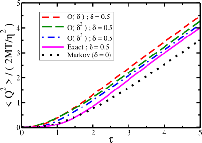
Figure 1: Normalized average quadratic dispersion of the quantum particle $\langle Q^{2}\rangle$ as a function of the dimensionless time $\tau=(\eta/M)t$ for $\delta=0.5$. The usual Markovian result (black, dotted line) is compared to the behavior in the presence of non-local corrections up to order $\sim\delta$, $\sim\delta^{2}$ and $\sim\delta^{3}$ (dashed lines, top to bottom, respectively), as well as with the exact non-Markovian Brownian evolution (magenta, solid line).

Notice also that the exact result lies between the Markovian and the approximate non-Markovian results. Such a counterintuitive behavior can be interpreted as a consequence of the effectively diminished mass that guides the truncated non-Markovian evolution, especially at early times: $\overline{M}\equiv M+2\eta J_{1}/\Omega$. The effective inertia of the non-Markovian Brownian particle described by the lowest non-trivial order of our truncated systematic expansion is clearly smaller than in the corresponding Markovian approximation, yielding therefore larger quadratic dispersions. Higher-order non-Markovian terms bring about higher derivatives $Q^{(n)}$ in the evolution equation that contribute eventually to the quantitative correction of this trend, approaching the exact result. It is interesting to note that this is a general feature of the $O(\delta)$ result, regardless of which explicit memory kernel is being considered. Since the integral $J_{1}$ is always negative (cf. Eq. (44)), the effective mass $\overline{M}\equiv M+2\eta J_{1}/\Omega$ is always smaller than the original one. Provided that the $O(\delta)$ non-white noise does not compete with the reduced effective inertia, the average quadratic dispersion will be increased in the truncated non-Markovian case. For the case of an exponential kernel, Fig. 1 shows that the first non-trivial order of our truncated systematic expansion is in fact an overestimate of the Non-Markovian effects in the quadratic dispersion.

Fig. 2 displays the late-time behavior of $\langle Q^{2}\rangle$ for different values of $\delta$: $0$ (local), $0.1$ and $0.3$ (non-local). It illustrates the modifications brought about by the first non-trivial corrections in our expansion for reasonable (not too large) values of $\delta$. The normalization is given by the Markovian late-time limit, Eq. (65). All curves flatten out for large enough times, as expected, with the late-time behavior being exactly the same.

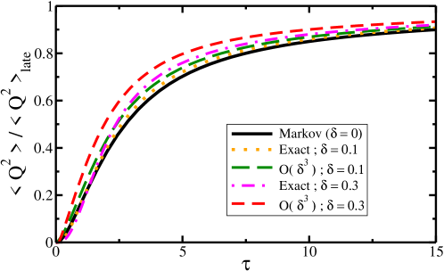
Figure 2: $\langle Q^{2}\rangle$ normalized by the Markovian late-time behavior, Eq. (65), as a function of the dimensionless time $\tau=(\eta/M)t$. The Markovian approximation ($\delta=0$) is compared to the exact and truncated (up to $O(\delta^{3})$) non-Markovian results for different values of $\delta=\eta/M\Omega$.

Using the systematic non-local expansion presented in the previous section, one can then estimate analytically the deviation from a Markovian behavior of the early-time dynamics of a given system straightforwardly. For instance, this can be used as a prescription for evaluating the importance of transient effects generated by non-Markovian corrections on the dynamics of the system under investigation to decide whether it is worth the effort of incorporating them in a full numerical simulation. Conversely, it can be used to incorporate memory effects order by order in $\delta=\eta/M\Omega$ without the need of performing a full memory integral in each time step of a simulation.

VI Conclusions and outlook

The complex structures of memory kernels, which usually can be cast into non-trivial dissipation and noise terms in a Langevin evolution equation, can not be disregarded even as a first approximation in several systems of interest in condensed matter, as well as in nuclear and particle physics under extreme conditions. Subdiffusion problems in chemical and biological systems and non-Abelian plasmas are just a few examples of this wide class of phenomena. In most cases, however, the incorporation of non-local effects is either overlooked or performed uniquely via numerical computation. The latter usually demands heavy computer power and has the caveat of not providing the type of insight that one can extract from analytic calculations, even within a simple framework.

In this paper we presented a systematic semi-analytic method that can be combined effectively with numerical techniques to tackle the non-Markovian Langevin evolution of a dissipative dynamical system in quantum mechanics. Making use of the Schwinger-Keldysh formalism within the path integral framework, we discussed the physics content of the frequency cutoff for the interaction of the system with the heat bath, which is commonly taken for granted in the usual Caldeira-Leggett description of open systems in quantum mechanics. We considered the kernel and noise correlator that follow from the most common choices, and also some less frequent, and derived an analytic expansion for the exact non-Markovian dissipation kernel and the corresponding colored noise for a general potential that is consistent with the fluctuation-dissipation theorem and incorporates systematically non-local corrections.

Using the non-Markovian Brownian motion with an exponential kernel, we illustrated how to implement the method and showed its consistency in recovering the relevant and well-known limits. This technique can be applied to any kernel that is amenable to a series expansion of the sort performed in this paper, which represents a very wide class of possibilities for applications. We believe that a combination of the semi-analytic treatment proposed in this paper with regular numerical methods can be of use in the study of several physical systems, at least providing shortcuts for numerical calculations and reasonable estimates for the relevance of non-local corrections given the typical scales of the problem under consideration.

Although the Laplace method is much more limited in the case of nonlinear equations, as will be the case once one goes beyond the harmonic approximation for the external potential, it is of great power for the Brownian problem with memory. For an external potential of generic form one can avoid the Laplace method at the cost of introducing higher order time derivatives. With the method presented in this work, one can address pragmatically several physical systems that exhibit this behavior, as was discussed in the introduction. The extension to quantum field theory is certainly not trivial, but possible.

References

- (1) R. Kubo, M. Toda and N. Hashitsume, Statistical Physics II - Nonequilibrium Statistical Mechanics (Sringer-Verlag, 1998).
- (2) U. Weiss, Quantum Dissipative Systems, 2nd edition (World Scientific, 1999).
- (3) E. A. Calzetta and B.-L. B. Hu, Nonequilibrium Quantum Field Theory (Cambridge, 2008).
- (4) J. D. Gunton, M. San Miguel and P. S. Sahni, in Phase Transitions and Critical Phenomena (Eds.: C. Domb and J. L. Lebowitz, Academic Press, London, 1983), v. 8.
- (5) Procs. of Quark Matter 2008, J. Phys. G 35 100301-109901 (2008).
- (6) D. J. Schwarz, Annalen Phys. 12, 220 (2003); D. Boyanovsky, H. J. de Vega and D. J. Schwarz, Ann. Rev. Nucl. Part. Sci. 56, 441 (2006).
- (7) E. S. Fraga and G. Krein, Phys. Lett. B 614, 181 (2005); E. S. Fraga, G. Krein and R. O. Ramos, AIP Conf. Proc. 814, 621 (2006).
- (8) E. S. Fraga, T. Kodama, G. Krein, A. J. Mizher and L. F. Palhares, Nucl. Phys. A 785, 138 (2007); E. S. Fraga, G. Krein and A. J. Mizher, Phys. Rev. D 76, 034501 (2007); G. Ananos, E. S. Fraga, G. Krein and A. J. Mizher, AIP Conf. Proc. 892, 396 (2007).
- (9) O. Scavenius, A. Dumitru, E. S. Fraga, J. T. Lenaghan and A. D. Jackson, Phys. Rev. D 63, 116003 (2001).
- (10) A. Bessa, E. S. Fraga and B. W. Mintz, Phys. Rev. D 79, 034012 (2009).
- (11) M. Gleiser and R. O. Ramos, Phys. Rev. D 50, 2441 (1994).
- (12) C. Greiner and B. Muller, Phys. Rev. D 55, 1026 (1997).
- (13) D. H. Rischke, Phys. Rev. C 58, 2331 (1998).
- (14) J. Berges, AIP Conf. Proc. 739, 3 (2005).
- (15) R. L. S. Farias, R. O. Ramos and L. A. da Silva, Braz. J. Phys. 38, 499 (2008).
- (16) P. Hänggi, Generalized Langevin Equations: A Useful Tool for the Perplexed Modeller of Non-equilibrium Fluctuations, Lecture Notes in Physics Vol. 484, Springer, Berlin, 1997, pp. 15 22.
- (17) D. Vollhardt and P. Wölfle, Phys. Rev. Lett. 45, 842 (1980); Phys. Rev. B 22, 4666 (1980).
- (18) A. H. Lo and C. McKinley, A Non-Random Walk Down Wall Street, Princeton University Press, Princeton, NJ, 1999.
- (19) S. Picozzi and B.J. West, Phys. Rev. E 66, 046118 (2002).
- (20) H. Yang, G. Luo, P. Karnchanaphanurach, T-M. Louie, I. Rech, S. Cova, L. Xun, and X.S Xie, Science 302, 262 (2003).
- (21) W. Min, G. Luo, B. J. Cherayil, S. C. Kou, and X. S. Xie, Phys. Rev. Lett. 94, 198302 (2005).
- (22) R. P. Feynman and Hibbs, Quantum Mechanics and Path Integrals (McGraw-Hill, 1965).
- (23) H. Kleinert, Path Integrals in Quantum Mechanics, Statistics, Polymer Physics, and Financial Markets (World Scientific, Singapore, 2004).
- (24) G. E. Uhlenbeck and L. S. Ornstein, Phys. Rev. 36, 823 (1930).
- (25) A. O. Caldeira and A. J. Leggett, Physica 121A, 587 (1983).
- (26) H. Grabert, P. Schramm and G. L. Ingold, Phys. Rept. 168, 115 (1988).
- (27) B. L. Hu, J. P. Paz and Y. h. Zhang, Phys. Rev. D 45, 2843 (1992); 47, 1576 (1993).
- (28) R. P. Feynman and F. L. Vernon, Annals Phys. 24, 118 (1963) [Annals Phys. 281, 547 (2000)].
- (29) G. W. Ford, M. Kac and P. Mazur, J. Math. Phys. 6, 504 (1965).
- (30) A. O. Caldeira and A. J. Leggett, Phys. Rev. Lett. 46, 211 (1981); Annals Phys. 149, 374 (1983).
- (31) J. Schwinger, J. Math. Phys. (N.Y.) 2, 407 (1961); P. M. Bakshi and K. T. Mahanthappa, J. Math. Phys. (N.Y.) 4,1 (1963); 4, 12 (1963); L. V. Keldysh, Zh. Eksp. Teor. Fiz. 47, 1515 (1964).
- (32) K. Chou, Z. Su, B. Hao and L. Yu, Phys. Rep. 118, 1 (1985); N. P. Landsman and C. G. van Weert, Phys. Rept. 145, 141 (1987).
- (33) J. P. Sethna, Phys. Rev. B 24, 698 (1981).
- (34) M. Abramowitz and I. A. Stegun (eds.), Handbook of Mathematical Functions (Dover, New York, 1965).
- (35) T. Koide, G. Krein and R. O. Ramos, Phys. Lett. B 636, 96 (2006).
- (36) R. L. S. Farias, N. C. Cassol-Seewald, G. Krein and R. O. Ramos, Nucl. Phys. A 782, 33 (2007).
- (37) R. L. S. Farias, Rudnei O. Ramos and L.A. da Silva, Comp. Phys. Comm. 180, 574 (2009).