Random fluctuation leads to forbidden escape of particles
Phys. Rev. E 82 026211 (2010)

Abstract

A great number of physical processes are described within the context of Hamiltonian scattering. Previous studies have rather been focused on trajectories starting outside invariant structures, since the ones starting inside are expected to stay trapped there forever. This is true though only for the deterministic case. We show however that, under finitely small random fluctuations of the field, trajectories starting inside Arnold-Kolmogorov-Moser (KAM) islands escape within finite time. The non-hyperbolic dynamics gains then hyperbolic characteristics due to the effect of the random perturbed field. As a consequence, trajectories which are started inside KAM curves escape with hyperbolic-like time decay distribution, and the fractal dimension of a set of particles that remain in the scattering region approaches that for hyperbolic systems. We show a universal quadratic power law relating the exponential decay to the amplitude of noise. We present a random walk model to relate this distribution to the amplitude of noise, and investigate this phenomena with a numerical study applying random maps.

Scattering is the general term used to describe systems whose dynamics take place in an unbounded phase space, and such that the dynamics is trivial outside of a localised region called the interaction region. A classical example is a thrown particle which collides or interacts with a fixed target, then escapes from the neighbourhood of the obstacle. If the region where such particle interacts with the obstacle is much smaller than the whole space we locally assume that the particle comes from infinity and is scattered again towards infinity. Alternatively, we may want to consider the dynamics of initial conditions starting inside the scattering region, in other words, the dynamics of an open system. We represent it by the dynamics, $x_{n+1}=f(x_{n})$, taking place in an unbounded phase space $M$ such that, the scattering region is $\textbf{W}\subset M$. Accordingly, the orbits of initial conditions in W, the region of interest, may eventually leave W permanently. When the dynamics within a scattering region is chaotic, we say that we have a chaotic scattering. A typical signature for chaotic scattering is that characteristic quantities associated with the particles, or trajectories, after being scattered are sensitive to their initial conditions before entering the scattering region.

Chaotic scattering is a very active research topic in dynamical systems. It has been found to describe a very broad class of dynamical processes. To mention a few cases, one may consider the dynamics of active chaos, i.e. chemical reagents or biological particles being advected by the flow and at the same time undergoing intrinsic transformations, such as biological reproduction or chemical reactions. A remarkable example is found in the study of plankton population in the oceans MoG04 ; TMG05 . One may also consider the dynamics of blood flow and investigate the role of the chaotic advection in the residence time of platelets and its consequence for the deposit and blocking of blood vessels SGM09 . A further example may be taken from the consideration of scattering particles in celestial dynamics saturn , among many other dynamical phenomena.

Because scattering dynamics are so closely related to scattering of particles in physical systems, we commonly refer to the dynamics of initial conditions in a region of the phase space as dynamical of particles whose dynamics started in such region. From the dynamics point of view, chaotic scattering is characterised by the presence of a chaotic non-attracting set containing periodic orbits of arbitrarily large periods as well as aperiodic orbits distributed on a fractal geometric structure in the phase space — the chaotic saddle Ott02 . In analogy to more general dynamics, chaotic scattering can be hyperbolic and non-hyperbolic. In the former case, all orbits in the chaotic saddle are unstable, and a randomly chosen initial condition has full probability of escaping within finite time. Hyperbolic scattering is also associated with an exponential decay of probability for particles to be found in the scattering region after a given time $t$. That is, if we have a number $N_{0}$ of randomly chosen initial conditions within the scattering region, the number of particles $N(t)$ in that region decays exponentially on time and consequently

$$P(t)\propto e^{-\kappa t},$$

where $P(t)=\lim_{N(0)\to\infty}N(t)/N(0)$ is the probability for particles to remain in the interaction region after time $t$ , and $\kappa$ a constant Ott02 . Non-hyperbolic scattering, on the other hand, is characterised by the presence of Kolmogorov-Arnold-Moser (KAM) islands in phase space. These islands surround marginally stable periodic orbits. Orbits from the outside can spend a long time in the vicinity of the KAM islands before escaping, and this “stickiness” effect causes a slower escape dynamics than that found in hyperbolic systems: non-hyperbolic escape is characterised by a power law distribution of probability,

$$P(t)\propto t^{-\alpha},$$

for large enough $t$ L-F-OttPRL91 ; MotterPRE01 ; MotterPRE03 . An important characteristic is that due to the invariance of the islands and the area preserving property of the dynamics, if initial conditions are chosen inside an island, orbits are expected to be trapped there forever Ott02 .

The above discussion refers to completely deterministic dynamics. However, since most phenomena in nature are always subjected to small fluctuations from their surrounding environment, a central question is: how does the dynamics of scattering systems change in the presence of random perturbations?

Here we focus on random perturbations of the parameters defining the system. From the Dynamical Systems perspective, this situation can be formalised by the concept of random maps, which we will apply throughout this paper,

$$x_{n+1}=f_{n}(x_{n}),$$

where we randomly choose slightly different maps $f_{n}$ for each iteration $n$ (see Eq. 2 below). It is known that such dynamics has well-defined (in the ensemble sense) values of dynamical invariants such as fractal dimensions and Lyapunov exponents Fal86 ; Arn98 ; RGO90 . Note that we associate the choice of the map with the iteration. Therefore, all initial conditions in a given iteration are mapped by the same sequence of random maps. On the other hand, if we implement independent random noise added to each trajectory, what has been previously considered for the random noisy dynamics PoG95 ; FeG97 ; SHS09 ; KrG04 ; KrG04b , the situation is very different, as we shall discuss later.

Let us recall that hyperbolicity is a structurally stable characteristic of dynamical systems, i.e. hyperbolic systems are robust under small smooth perturbations of the system. But on general grounds, one expects the perturbation of a non-hyperbolic dynamical system to result in a hyperbolic dynamics. We remark that the notion of structural stability is related to perturbations of the whole dynamical system and not to noisy diffusion-like perturbations of individual trajectories Rob99 . Although it is possible to define random invariants in more general grounds Arn98 , for our context it makes no sense to talk about dynamical invariants such as the Lyapunov exponent and fractal dimensions in the noisy dynamics in this latter case, because trajectories will be “smoothed-out” in small scales and all fine-structure dynamical structures will disappear. In the case of perturbation of parameters, on the other hand, we have “random maps”RGO90 , which are known to have well-defined dynamical invariants in a measure-theoretical senseFal86 .

A further observation is that, since hyperbolic systems are structurally stable, we expect that small perturbations would not result in qualitative changes to the dynamics of hyperbolic maps. In particular, escape should continue to be exponential. For non-hyperbolic systems, the same can not be expected. Thus, we expect to see qualitative changes due to the perturbations. As an example, we could heuristically see the KAM tori no longer as confining, since now the perturbations can always push orbits out of the region of an island, and conversely orbits on the outside can be pushed inside a torus by the perturbations. The destruction of this essential feature of non-hyperbolic scattering leads us to hypothesise that even arbitrarily small random perturbations to the dynamics will turn a non-hyperbolic scattering system into a hyperbolic-like dynamics. Hence, we expect the probability distribution of escaping time for perturbed non-hyperbolic systems to become exponential.

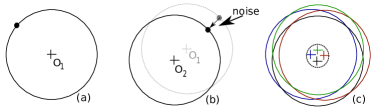
Figure 1: (Colour online) Simplified representation of the orbits on the torus. In (a), it is represented a single torus and its centre. In (b), it is represented the effect of the perturbation. The difference between the dashed and the continuous line is due to the effect of the noise, that deslocate the centre of the torus from $O_{1}$ to $O_{2}$. In (c) we show what would be expected for $4$ iterations. Each continuous line represents the orbit of a particle on the torus for each iteration, hence different values of perturbations at each iteration. The centre is expected to move around $O_{1}$ at each iteration and for long enough time, the distribution of centres would fill densely the area within the dashed circle.

In this paper we explore and test this hypothesis using a simple scattering map as a model system. We derive an analytical theory to predict the scaling of the escape rate of non-hyperbolic scattering systems under weak perturbations. The theory predicts that the (exponential) escape rate goes to zero as the amplitude of the perturbation decreases following a quadratic law, which we argue is universal for all perturbed non-hyperbolic systems. We verify this prediction numerically, and find that it describes well the results of our simulations.

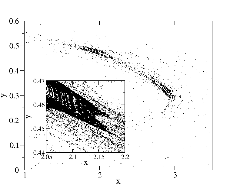
Figure 2: Phase space for the map 2, for $\lambda=6.0$. The inset shows a blowup of the region $(x,y)\in[2.05,2.20]\times[0.44,0.47]$.

In order to better understand the effects of random parameter perturbations on the dynamics of non-hyperbolic Hamiltonian systems, we develop now a simple statistical model of the motion of a single trajectory in the presence of perturbations.

In the absence of random perturbations, the islands act as barriers in the phase-space; Due to the area-preserving property of such dynamics, those invariant structures can not be transposed Ott02 , thus trajectories trapped inside islands never escape. Now suppose a small noise is added to the system’s parameter. The effect of noise is to vary randomly the parameter from iteration to iteration, but noise amplitude is assumed to be small enough so that the parameter lies in the range where the system is non-hyperbolic. The effect of one iteration could be, say, to change the parameter $\lambda$ to a slightly smaller value, but still keep it within the range such that the dynamics is non-hyperbolic. The effect of the new parameter is then to cause a small shift in the KAM structures compared to the value of $\lambda$ in the previous iteration. For the next iteration another value of $\lambda$ is chosen, and the KAM islands again move slightly in phase-space. This happens at every iteration, and the global effect is a sort of random walk of the KAM structures around their positions in the absence of noise. Fig 1 is an idealised illustration of the orbit of a particle on a torus. We represented three steps, a simple torus - Fig 1 (a)-, the effect of the new parameter - Fig 1 (b) -, and finally, what would be ideally expected for 4 iterations - Fig 1 (c).

In other words, the perturbations can be imagined to cause orbits to gain motion in the direction transversal to the tori. The magnitude of this transversal component of the motion is proportional to the intensity of the perturbation (in the case of small perturbations). Since only the transversal component can cause an orbit started within a KAM island to escape, we focus on this component of the motion alone.

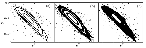
Figure 3: KAM structures under the perturbed dynamics for different values of $\xi$. Fig 3(a), $\xi=0$, Fig 3(b), $\xi=0.0004$, and Fig 3(c), $\xi=0.002$.

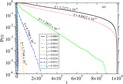
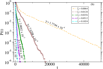
Figure 4: (colour online) Probability distribution of escaping time $t$ from the region $\boldsymbol{W}=\{|x|<5.0,\quad and\quad|y|<5.0\}$ for different values of $\xi$. Initial conditions were randomly chosen in the line $x\in[2.05,2.07],y=0.465$ inside nest KAM structures. For each value of $\xi$, we present the exponent $\gamma$ that best fits the exponential region of the probability distribution. Fig 4(a) shows all used values of $\xi$, Fig 4(b), shows small values of $t$.

The transversal motion is due entirely to the random perturbations, and as a first approximation we model it as a one-dimensional random walk. The size of the step $\delta$ of the random walk is proportional to the amplitude of the perturbation. After $n$ steps, the typical distance $D$ from the starting position reached by the walker is $D\sim\sqrt{n}\delta$ Feller . Let $D_{0}$ be a typical transversal distance a particle needs to traverse in order to cross the last KAM surface and escape. Thus the average time (number of steps) $\tau$ it takes for particles to escape scale is given by $D_{0}^{2}\sim\tau\delta^{2}$. So $\tau$ scales as $\tau\sim\delta^{-2}$. The conclusion is that our simple model predicts an exponential decay of particles, with a decay rate $\kappa\sim\tau^{-1}$ scaling as

$$\kappa\sim\delta^{2}.$$ (1)

Note that the dynamics described by random maps here is very different from that where random noise is added to individual trajectories. In the latter case, an analysis in terms of stochastic stability is more adequate, because the behaviour of, for example, two distinct orbits evolved from different initial conditions cannot be compared in terms of (Lyapunov) stability. In fact, even by following two distinct time evolutions from the same initial condition we may observe completely distinct behaviour due to the two different noise realisations, possibly not correlated. In particular, for scattering under the presence of noise SHS09 , it has been shown that the exponential escape rate is preserved in weakly dissipative systems and that also an exponential escape rate should be expected for non dissipative ones, for noise intensity above a threshold. Indeed, because trajectories under different noise realisations may not be correlated for a certain level of noise, we expect a resultant random behaviour to be dominant, and therefore a distribution of random values of escaping time. Hence, an exponential distribution naturally follows. This scenario has already been pictured in SHS09 by considering that above the critical level of noise, an effective random redistribution of particles results in a blurring of the fine structure of the KAM tori. In the dynamics given by random maps considered here, on the other hand, all the trajectories are evolved under the same realisation and fine-scale structures are preserved for each map, allowing a well-defined analysis of structural properties of limit sets Arn98 . In this case, one can, for example, evaluate the Lyapunov stability of orbits by comparing the convergence towards one another or the divergence of different random orbits generated by the evolution of distinct initial conditions, since they are subject to the same sequence of perturbations. It is also possible to define consistently the fractal dimension of invariant sets under the iteration of the random maps Fal86 , unlike in the case of independent realizations of noise for different particles. Intuitively, we can think of such a system as perturbations of the dynamics itself, for example, a set of particles that evolve subject to a field that undergoes random fluctuations. Therefore, all particles are thought to evolve under the same sequence of dynamical laws, rather than each particle being subject to random uncorrelated kicks. This key characteristic is what allows us to consider our model based on the random walk of the tori and develop our approach in order to derive the power law described by equation 1. As we shall see in what follows, it also allows us to consider singular sets of initial conditions, which we will use to compute the fractal dimension. Furthermore, we remark again that the initial conditions used here are always chosen inside the original KAM structures. For this set of particles, if no random perturbation is considered, there should not have any escape at all due to the are preserving property of our map. Simply the fact that such escape indeed happens is already by itself a novelty characteristic introduced by the perturbations of the dynamics and explained by our theory.

In order to test our theory, we numerically obtained the probability distribution $P(t)$ that particles have not escaped at time $t$ from a given region $\boldsymbol{W}$ of the phase-space under the dynamics of an area-preserving non-hyperbolic map. We have chosen the map

$$\begin{split}x_{n+1}&=\lambda_{n}[x_{n}-(x_{n}+y_{n})^{2}/4]\\ y_{n+1}&=\frac{1}{\lambda_{n}}[y_{n}+(x_{n}+y_{n})^{2}/4],\end{split}$$ (2)

which is non-hyperbolic for $\lambda\lesssim 6.5$ L-F-OttPRL91 . We define $\boldsymbol{W}=\{|x|<5.0,|y|<5.0\}$. The initial conditions were randomly chosen with uniform probability in the line $x\in[2.05,2.07],y=0.465$. For this interval, the particles start their trajectories inside a KAM structure (See Fig 2). Because we are interested in perturbing the system, we chose $\lambda^{*}=6.0$. Then, for each iteration $n$ we randomly chose a perturbation $|\varepsilon_{n}|$ in the interval $|\varepsilon_{n}|<\xi$, where $\xi$ is the amplitude of the perturbation. Indeed, for the simulations we observe, as expected, the scenario pictured in Fig. 1. We show in Fig. 3 a portion of the phase space containing KAM islands for different values of perturbations.

We show in Fig 4 the probability distribution $P(t)$ for different values of $\xi$. We clearly see that the escape follows an exponential law in a broad range of times, for various perturbation amplitudes. For each value of $\xi$, we show the exponent $\gamma$ that best fits the exponential law $P(t)\sim e^{-\gamma t}$ in the range of times for which the probability distribution is exponential.

We also observe that for small values of the perturbation amplitude, the stickiness plays an important role on the escaping time distribution of particles that leave the non-attracting chaotic set. This is because even after a particle escapes from a KAM island, it may be trapped for long times by Cantori. Under small amplitude of perturbations, this causes a slower escape than that predicted by our model. This signature of the stickiness is observed in the tail of the distribution shown in Fig. 4 as a cutoff for long times in the exponential escape of particles. The exponential probability distribution of escape time agrees with our hypothesis that the dynamics of the perturbed system is hyperbolic-like in the presence of the random perturbations.

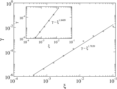
Figure 5: Different values of exponent $\gamma$ as a function of $\xi$ from Fig. 4, as well as the power law that best fits the distribution. In the inset, we consider only values of $\xi<0.02$.

Using our random walk escaping model, from Eq. 1 and Fig. 5, we identify $\kappa\equiv\gamma$, and $\delta\equiv\xi$. In order to construct our model, we have not taken into account the effect of stickiness. Therefore, it is reasonable to expect that the obtained exponent should actually be smaller than $2$. We show in Fig. 5 the dependence of $\gamma$ on the amplitude of the perturbation $\xi$, for the map given by Eq. (2). First of all, we notice that $\gamma$ indeed follows a power-law, as our model predicts. We also obtained a good agreement with the square law predicted by Eq. 1.

Another fundamental characteristic, differentiating non-hyperbolic chaotic scattering from the hyperbolic case, is the fractal dimension of singular sets. One expects that choosing initial conditions from a line in $\boldsymbol{W}$, the set of particles that remain in $\boldsymbol{W}$ after a given time $T_{0}$ should form a Cantor set with fractal dimension $d<1$ in the case of hyperbolic dynamics. It is due to the exponential decay of probability, characteristic of hyperbolic systems. On the other hand, the algebraic decay of non-hyperbolic scattering leads to the maximal value of the fractal dimension, $d=1$ L-F-OttPRL91 . However, it is well known that in practice one would need in most cases to go down to unreasonably small scales to see the actual $d=1$ prediction in a non-hyperbolic scattering system. For scales that are physically meaningful, in most cases one finds that the chaotic saddle and its associated sets (stable and unstable manifolds, etc.) have a position-dependent effective dimension MoG04 ; MotterPRE03 , which is lower than $1$.

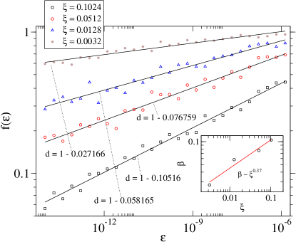
Figure 6: (colour online) Estimated fractal dimension of the $T$, for different values of $\xi$. We notice that, when the amplitude of the perturbation is decreased, the dynamics approach the non-hyperbolic limit, and so does the estimated values of fractal dimension. The inset shows the value of $\beta$ as a function of $\xi$.

As an example of scattering function, we consider the time-delay $T(x)$. The idea is to calculate the fraction $f(\varepsilon)$ of pairs of initial conditions started in random positions of the phase space with distance $\varepsilon$ of each other whose trajectories diverge within the scattering region, and whose orbits end up escaping through completely different routes. In order to compute that, we chose initial conditions inside a KAM structure. We chose $y_{0}=0.465$, and different values of $x_{0}$ were randomly chosen to belong to the interval $[2.05,2.15]$. For a fixed value of uncertainty $\varepsilon$ we chose $x_{0}$ and compute $|T(x_{0})-T(x_{0}+\varepsilon)|$. If $|T(x_{0})-T(x_{0}+\varepsilon)|>2$ we say that $x_{0}$ is $\varepsilon$-uncertain. Dividing the number of $\varepsilon$-uncertain points by the total number of initial conditions we obtain $f(\varepsilon)$, the uncertain fraction. It can be shown that for chaotic scattering systems $f(\varepsilon)$ scales as a power law $\varepsilon^{\beta}$, and that the box-counting fractal dimension $d$ is given by $d=1-\beta$ grebogi83 . We expect that the smaller the amplitude of noise, the closer the $d$ is to $1$, which would correspond to the non-hyperbolic limit. We show in Fig. 6 the estimated fractal dimension of the function $T(x)$, for different values of $\xi$. We notice that when the amplitude of the perturbation is decreased, the dynamics approach the non-hyperbolic limit, and so do the estimated values of fractal dimension, which approach 1 as $\xi\rightarrow 0$. Furthermore, we notice that $\beta$ scales as a power law with the amplitude of noise, i.e. $\beta\sim\xi^{0.37}$.

In conclusion, we have shown that random small perturbation of non-hyperbolic maps leads to hyperbolic behaviour. We have presented a random walk model to explain the escape of particles from inside invariant KAM islands. Such particles are expected to be trapped there forever in the absence of perturbation. When the perturbation is present, we show that, not only particles are able to escape, but also they have hyperbolic behaviour, with a universal quadratic power law relating the exponential decay to the amplitude of the perturbation. We further investigated the hyperbolic behaviour estimating the fractal dimension of the set of particles that remain inside the islands for a given time. We show that indeed the fractal dimension is in agreement to what is expected for a hyperbolic system.

We call the attention of the reader to an important issue on scattering dynamics clarified by our results. Note that despite the generality of scattering phenomena, mostly of the modelling of real processes has assumed a simpler chaotic dynamics, that is, given by hyperbolic structures. Nevertheless, it is widely argued that most of the flows experimentally significant are non-hyperbolic; see references therein MoG04 . In active dynamics, or blood flow, for example, the modelling describe systems where we have trapped vortices. Therefore, in the absence of perturbations the particles would not leave the trapping regions; This would correspond to plankton not being able to leave a given region in the sea, or blood particles being trapped indefinitely in vortices, which is in contrast with most observations. As a consequence, although the dynamics is described by non-hyperbolic scattering, the escape is in many cases assumed to follow an exponential law, without any further explanation TMG05 ; SGM09 . Since it is reasonable to assume that these flows naturally experience random perturbations, our theory provides an important bridge to allow one to encompass natural phenomena under the non-hyperbolic scattering framework.

Apart from striking implications to the above mentioned dynamics, our result may play a fundamental role on the understanding of how sources, and escaping rates of particles act on the dynamics of Saturn Rings saturn . The rings are thought to be marginally stable periodic orbits, and the gaps to be rational tori or made up by commensurable frequencies. They are subjected to gravitational perturbation and perturbations of the electromagnetic field, due to solar storms, solar winds, magnetic storms, etc. saturn , or due to the dynamic of ring current around Saturn saturn . Such random perturbations would be represented by our perturbation on the parameter $\lambda$ in Eq. 2. Hence, if measured, we would expect an exponential-like escape of particles. Therefore our results may shed some light onto the understanding of the escape of small particles like in the Saturn’s E ring saturn .

References

- (1) T. Tel, A. de Moura, C. Grebogi, and G. Karolyi Phys. Report 413, 91 (2005).
- (2) A. P. S. de Moura, and C. Grebogi Phys. Rev. E 70, 36216 (2004).
- (3) A. B. Schelin, Gy. Károlyi, A. P. S. de Moura, N. A. Booth, and C. Grebogi, Phys. Rev. E 80, 016213 (2009).
- (4) G. H. Jones, et al., Science 319, 1380 (2008);B. Sicard, Space Science Rev. 116, 457 (2005); C. D. Murray, et al., Nature 437, 1326 (2005); R. Karjalainen, and H. Salo, Icarus 172, 328 (2004); E. Grun, et al., Icarus 54, 227 (1983); V. V. Dikarev, et al., Planetary and Space Science 54, 1014 (2006); K. Ohtsuki, The Astrop. Journ. 626, L62 (2005); Frank Spahn, et al., Science 311, 1416 (2006); See Sec. in M. V. Berry - ’Regular and Irregular Motion’ in Topics in Nonlinear Mechanics - ed. S Jorna, Am.Inst.Ph.Conf.Proc Introduction to chaos and coherence , IOP(1992), and references therein; S. M. Krimigis, et al., Nature 450, 1050 (2007).
- (5) E. Ott, Chaos in Dynamical Systems 2ed. (Cambridge University Press, Cambridge, UK 2002).
- (6) A. E. Motter and Y.-C. Lai, Phys. Rev. E 65, 015205 (2002).
- (7) Y. T. Lau and J. M. Finn and E. Ott, Phys. Rev. Lett 66, 978 (1991).
- (8) A. E. Motter and Y.-C. Lai and C. Grebogi, Phys. Rev. E 68, 056307 (2003).
- (9) L. Arnold, Random dynamical systems., Springer-Verlag(1998).
- (10) L. Poon and C. Grebogi. Phys. Rev. Lett, 75: 4023, 1995.
- (11) U. Feudel, and C. Grebogi. Chaos, 7: 597, 1997.
- (12) J. M. Seoane, L. Huang, M. A. F. Suanjuan and Y.-C. Lai, Phys. Rev. E 79, 047202 (2009).
- (13) S. Kraut and C. Grebogi, Phys. Rev. Lett. 92, 234101 (2004).
- (14) S. Kraut and C. Grebogi, Phys. Rev. Lett. 93, 250603 (2004).
- (15) C. Robinson, Dynamical Systems: Stability, Symbolic Dynamics, and Chaos 2ed., (CRC Press, FL 1999).
- (16) F. J. Romeiras, C. Grebogi and E. Ott, Phys. Rev. A 41, 784 (1990).
- (17) K. J. Falconer, The Geometry of Fractal Sets (Cambridge University Press, Cambridge, UK 1986).
- (18) W. Feller, Introduction to probability theory and applications , Wiley(2001).
- (19) C. Grebogi, S. W. McDonald, E. Ott, and J. A. Yorke, Phys. Lett 99A, 415 (1983).