Non-perturbative QCD effective charges

Abstract

Using gluon and ghost propagators obtained from Schwinger-Dyson equations (SDEs), we construct the non-perturbative effective charge of QCD. We employ two different definitions, which, despite their distinct field-theoretic origin, give rise to qualitative comparable results, by virtue of a crucial non-perturbative identity. Most importantly, the QCD charge obtained with either definition freezes in the deep infrared, in agreement with theoretical and phenomenological expectations. The various theoretical ingredients necessary for this construction are reviewed in detail, and some conceptual subtleties are briefly discussed.

1 Introduction

One of the challenges of the QCD is the self-consistent and physically meaningful definition of an effective charge. This quantity provides a continuous interpolation between two physically distinct regimes: the deep ultraviolet (UV), where perturbation theory works well, and the deep infrared (IR), where non-perturbative techniques, such as lattice or SDEs, must be employed. The effective charge depends strongly on the detailed dynamics of some of the most fundamental Green’s functions of QCD, such as the gluon and ghost propagators [1].

In this talk we will focus on two characteristic definitions of the effective charge, frequently employed in the literature. Specifically we will consider (i) the effective charge of the pinch technique (PT) [2, 3] and (ii) the one obtained from the ghost-gluon vertex [4].

2 Two non-perturbative effective charges

We first introduce the notation and the basic quantities entering into our study. In the covariant renormalizable ($R_{\xi}$) gauges, the gluon propagator $\Delta_{\mu\nu}(q)$ has the form

$$\Delta_{\mu\nu}(q)=-i\left[P_{\mu\nu}(q)\Delta(q^{2})+\xi\frac{q_{\mu}q_{\nu}}{q^{4}}\right],$$ (1)

where $\xi$ denotes the gauge-fixing parameter, $P_{\mu\nu}(q)=g_{\mu\nu}-q_{\mu}q_{\nu}/q^{2}$ is the usual transverse projector, and $\Delta^{-1}(q^{2})=q^{2}+i\Pi(q^{2})$, with $\Pi_{\mu\nu}(q)=P_{\mu\nu}(q)\Pi(q^{2})$ the gluon self-energy. In addition, the full ghost propagator $D(q^{2})$ and its dressing function $F(q^{2})$ are related by $iF(q^{2})=q^{2}D(q^{2})$. The all-order ghost vertex will be denoted by ${\rm I}\Gamma_{\mu}(k,q)$, with $k$ representing the momentum of the gluon and $q$ the one of the anti-ghost; at tree-level ${\rm I}\Gamma^{(0)}_{\mu}(k,q)=-q_{\mu}$.

An important ingredient for what follows is the two-point function $\Lambda_{\mu\nu}(q)$ defined by [1, 5]

$$i\Lambda_{\mu\nu}(q) = \lambda\int_{k}H^{(0)}_{\mu\rho}D(k+q)\Delta^{\rho\sigma}(k)\,H_{\sigma\nu}(k,q),$$ (2)

$$= g_{\mu\nu}G(q^{2})+\frac{q_{\mu}q_{\nu}}{q^{2}}L(q^{2}),$$

where $\lambda=g^{2}C_{\rm{A}}$, $C_{\rm{A}}$ is the Casimir eigenvalue of the adjoint representation, and $\int_{k}\equiv\mu^{2\varepsilon}(2\pi)^{-d}\int\!d^{d}k$, with $d$ the dimension of space-time. $H_{\mu\nu}(k,q)$ is represented in Fig. 1, and its tree-level, $H_{\mu\nu}^{(0)}=ig_{\mu\nu}$. In addition, $H_{\mu\nu}(k,q)$ is related to ${\rm I}\Gamma_{\mu}(k,q)$ by

$$q^{\nu}H_{\mu\nu}(k,q)=-i{\rm I}\Gamma_{\mu}(k,q)\,.$$ (3)

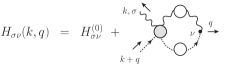
Figure 1: Diagrammatic representation of $H$.

2.1 The pinch technique effective charge

The PT definition of the effective charge relies on the construction of an universal (i.e., process-independent) effective gluon propagator, which captures the running of the QCD $\beta$ function, exactly as happens with the vacuum polarization in the case of QED [2, 6] (See Fig. 2).

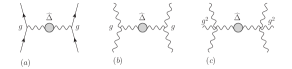
Figure 2: The universal PT coupling.

One important point, explained in detail in the literature, is the (all-order) correspondence between the PT and the Feynman gauge of the BFM  [2, 7]. In fact, one can generalize the PT construction [2] in such a way as to reach diagrammatically any value of the gauge fixing parameter of the BFM, and in particular the Landau gauge. In what follows we will implicitly assume the aforementioned generalization of the PT, given that the main identity we will use to relate the two effective charges is valid only in the Landau gauge.

To fix the ideas, the PT one-loop gluon self-energy reads

$$\widehat{\Delta}^{-1}(q^{2})=q^{2}\left[1+bg^{2}\ln\left(\frac{q^{2}}{\mu^{2}}\right)\right],$$ (4)

where $b=11C_{A}/48\pi^{2}$ is the first coefficient of the QCD $\beta$-function. Due to the Abelian WIs satisfied by the PT effective Green’s functions, the new propagator-like quantity $\widehat{\Delta}^{-1}(q^{2})$ absorbs all the RG-logs, exactly as happens in QED with the photon self-energy. Then, the renormalization constants of the gauge-coupling and of the PT gluon self-energy, defined as

$$g(\mu^{2}) = Z_{g}^{-1}(\mu^{2})g_{0},$$

$$\widehat{\Delta}(q^{2},\mu^{2}) = \widehat{Z}^{-1}_{A}(\mu^{2})\widehat{\Delta}_{0}(q^{2}),$$ (5)

where the “0” subscript indicates bare quantities, satisfy the QED-like relation ${Z}_{g}={\widehat{Z}}^{-1/2}_{A}$. Therefore, the product

$${\widehat{d}}_{0}(q^{2})=g^{2}_{0}\widehat{\Delta}_{0}(q^{2})=g^{2}(\mu^{2})\widehat{\Delta}(q^{2},\mu^{2})={\widehat{d}}(q^{2}),$$ (6)

forms a RG-invariant ($\mu$-independent) quantity [2]. For asymptotically large momenta one may extract from ${\widehat{d}}(q^{2})$ a dimensionless quantity by writing,

$${\widehat{d}}(q^{2})=\frac{\overline{g}^{2}(q^{2})}{q^{2}},$$ (7)

where $\overline{g}^{2}(q^{2})$ is the RG-invariant effective charge of QCD; at one-loop

$$\overline{g}^{2}(q^{2})=\frac{g^{2}}{1+bg^{2}\ln\left(q^{2}/\mu^{2}\right)}=\frac{1}{b\ln\left(q^{2}/\Lambda^{2}_{\scriptscriptstyle\mathrm{QCD}}\right)}.$$ (8)

where $\Lambda_{\scriptscriptstyle\mathrm{QCD}}$ denotes an RG-invariant mass scale of a few hundred ${\rm MeV}$.

Eq. (6) is a non-perturbative relation; therefore it can serve unaltered as the starting point for extracting a non-perturbative effective charge, provided that one has information on the IR behavior of the PT-BFM gluon propagator $\widehat{\Delta}(q^{2})$. Interestingly enough, non-perturbative information on the conventional gluon propagator $\Delta(q^{2})$ may also be used, by virtue of a general relation connecting $\Delta(q^{2})$ and $\widehat{\Delta}(q^{2})$. Specifically, a formal all-order relation known as “background-quantum” identity  [8] states that

$$\Delta(q^{2})=\left[1+G(q^{2})\right]^{2}\widehat{\Delta}(q^{2}).$$ (9)

Note that, due to its BRST origin, the above relation must be preserved after renormalization. Specifically, denoting by $Z_{\Lambda}$ the renormalization constant relating the bare and renormalized functions, $\Lambda_{0}^{\mu\nu}$ and $\Lambda^{\mu\nu}$, through

$$g^{\mu\nu}+\Lambda^{\mu\nu}(q,\mu^{2})=Z_{\Lambda}(\mu^{2})[g^{\mu\nu}+\Lambda_{0}^{\mu\nu}(q)],$$ (10)

then from (9) and ${Z}_{g}={\widehat{Z}}^{-1/2}_{A}$ follows the additional relation

$$Z_{g}^{-1}=Z_{A}^{1/2}Z_{\Lambda},$$ (11)

which is useful for the comparison with the coupling discussed in the following subsection.

It is now easy to verify, at lowest order, that the $1+G(q^{2})$ obtained from Eq. (2) restores the $\beta$ function coefficient in front of UV logarithm. In that limit [5]

$$1+G(q^{2}) = 1+\frac{9}{4}\frac{C_{\rm{A}}g^{2}}{48\pi^{2}}\ln\left(\frac{q^{2}}{\mu^{2}}\right),$$

$$\Delta^{-1}(q^{2}) = q^{2}\left[1+\frac{13}{2}\frac{C_{\rm{A}}g^{2}}{48\pi^{2}}\ln\left(\frac{q^{2}}{\mu^{2}}\right)\right].$$ (12)

Using Eq. (9) we therefore recover the $\widehat{\Delta}^{-1}(q^{2})$ of Eq. (4), as we should.

Then, non-perturbatively, one substitutes into Eq. (9) the $1+G(q^{2})$ and $\Delta(q^{2})$ obtained from either the lattice or SD analysis, to obtain $\widehat{\Delta}(q^{2})$. This latter quantity is the non-perturbative generalization of Eq. (4); for the same reasons explained above, the combination

$$\widehat{d}(q^{2})=\frac{g^{2}\Delta(q^{2})}{\left[1+G(q^{2})\right]^{2}}\,,$$ (13)

is an RG-invariant quantity.

2.2 The ghost-gluon vertex charge

In principle, a definition for the QCD effective charge can be obtained starting from the various QCD vertices; however, in general, such a construction involves more than one momentum scales, and further assumptions about their values need be introduced, in order to express the charge as a function of a single variable. The ghost-gluon vertex has been particularly popular in this context, especially in conjunction with Taylor’s non-renormalization theorem and the corresponding kinematics [4].

We next define the following renormalization constants

$$\Delta(q^{2})=Z^{-1}_{A}\Delta_{0}(q^{2}), F(q^{2})=Z^{-1}_{c}F_{0}(q^{2}),$$

$${\rm I}\Gamma^{\nu}(k,q)=Z_{1}{\rm I}\Gamma^{\nu}_{0}(k,q), g^{\prime}=Z_{g^{\prime}}^{-1}g_{0}\,.$$ (14)

Notice that a priori $Z_{g^{\prime}}$ defined as $Z_{g^{\prime}}=Z_{1}Z_{A}^{-1/2}Z_{c}^{-1}$, does not have to coincide with the $Z_{g}$ introduced in (5); however, as we will see shortly, they do coincide by virtue of the basic identity we will derive in next section.

It turns out that for the so-called Taylor kinematics (vanishing incoming ghost momentum, $k_{\mu}\to-q_{\mu}$), one may impose the additional condition

$$Z_{1}=Z_{g^{\prime}}Z_{A}^{1/2}Z_{c}=1\;\;\Rightarrow\;\;\ Z_{g^{\prime}}^{-1}=Z_{A}^{1/2}Z_{c}\,.$$ (15)

Thus, the combination

$$\widehat{r}(q^{2})\ =\ {g^{\prime}}^{2}\Delta(q^{2})F^{2}(q^{2})\,,$$ (16)

is a RG-invariant ($\mu$-independent) quantity. Therefore, for asymptotically large $q^{2}$, in analogy to Eq. (7) one can define an alternative QCD running coupling as

$$\widehat{r}(q^{2})=\frac{\overline{g}_{\mathrm{gh}}^{2}(q^{2})}{q^{2}}.$$ (17)

It is easy to verify that $\overline{g}^{2}_{\mathrm{gh}}(q^{2})$ and $\overline{g}^{2}(q^{2})$ displays the same one-loop behavior, since, perturbatively, the function $1+G(q^{2})$ is the inverse of the ghost dressing function $F(q^{2})$ (this is due to the general identity of Eq. 20).

3 An important identity

In this section, we discuss a non-trivial identity, valid only in the Landau gauge, relating the $F(q^{2})$ with the $G(q^{2})$ and $L(q^{2})$ of (2).

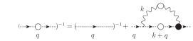
Figure 3: The SDE for the ghost propagator.

The derivation proceeds as follows. First, consider the standard SD equation for the ghost propagator, represented in Fig. 3, and written as

$$iD^{-1}(q^{2})=q^{2}+i\lambda\int_{k}\Gamma^{\mu}\Delta_{\mu\nu}(k){\rm I}\Gamma^{\nu}(k,q)D(p),$$ (18)

where $p=k+q$. Then, contract both sides of the defining equation (2) by the combination $q^{\mu}q^{\nu}$ to get

$$[G(q^{2})+L(q^{2})]q^{2}\!\!=\!\!\lambda\!\!\int_{k}\!\!q_{\rho}\Delta^{\rho\sigma}(k)\,q^{\nu}H_{\sigma\nu}(k,q)D(p).$$ (19)

Using the Eq. (3) and the transversality of the full gluon propagator, we can see that the rhs of Eq. (19) is precisely the integral appearing in the ghost SDE (18). Therefore, in terms of the ghost dressing function $F(q^{2})$,

$$1+G(q^{2})+L(q^{2})=F^{-1}(q^{2}).$$ (20)

Eq. (20), derived here from the SDEs, has been first obtained in [9], as a direct consequence of the BRST symmetry.

Let us study the functions $G(q^{2})$ and $L(q^{2})$ more closely. From Eq. (2) we have that (in $d$ dimensions)

$$G(q^{2}) = \frac{1}{(d-1)q^{2}}\left(q^{2}\Lambda_{\mu}^{\mu}-q^{\mu}q^{\nu}\Lambda_{\mu\nu}\right),$$

$$L(q^{2}) = \frac{1}{(d-1)q^{2}}\left(dq^{\mu}q^{\nu}\Lambda_{\mu\nu}-q^{2}\Lambda_{\mu}^{\mu}\right)\,.$$ (21)

In order to study the relevant equations further, we will approximate the two vertices, $H_{\mu\nu}$ and ${\rm I}\Gamma_{\mu}$, by their tree-level values, Then, setting $f(k,q)\equiv(k\cdot q)^{2}/{k^{2}q^{2}}$, one may show that [1]

$$F^{-1}(q^{2})\!\!\!\!\! = \!\!\!\!\!1\,\,+\,\,\lambda\!\int_{k}\!\![1\!\!-\!\!f(k,q)]\Delta(k)D(k+q),$$

$$(d-1)G(q^{2})\!\!\!\!\! = \!\!\!\!\!\lambda\!\int_{k}\!\![(d-2)\!\!+\!\!f(k,q)]\Delta(k)D(q+k),$$

$$(d-1)L(q^{2})\!\!\!\!\! = \!\!\!\!\!\lambda\!\int_{k}\!\![1\!\!-\!\!d\,f(k,q)]\Delta(k)D(q+k)\,,$$ (22)

It turns out that if $F$ and $\Delta$ are both IR finite, Eq. (22) yields the important result $L(0)=0$ [1].

Of course, all quantities appearing in Eq. (22) are unrenormalized. It is easy to recognize, for example, by substituting in the corresponding integrals tree-level expressions, that $F^{-1}(q^{2})$ and $G(q^{2})$ have exactly the same logarithmic dependence on the UV cutoff, while $L(q^{2})$ is finite at leading order.

Since the origin of (20) is the BRST symmetry, it should not be deformed after renormalization. To that end, using the definition of (10), in order to preserve the relation (20) we must impose that $Z_{\Lambda}=Z_{c}$. In addition, by virtue of (3), and for the same reason, we have that, in the Landau gauge, ${{\rm I}\Gamma}_{\nu}(k,q)$ and $H_{\sigma\nu}(k,q)$ must be renormalized by the same renormalization constant, namely $Z_{1}$ [viz. Eq. (14)]; for the Taylor kinematics, we have that $Z_{1}=1$ [see Eq. (15)] (for some additional subtleties see [1]).

Returning to the effective charges, first of all, comparing Eq. (6) and Eq. (16), it is clear that $g(\mu)=g^{\prime}(\mu)$, by virtue of $Z_{\Lambda}=Z_{c}$. Therefore, using Eq. (9), one can get a relation between the two RG-invariant quantities, $\widehat{r}(q^{2})$ and $\widehat{d}(q^{2})$, namely

$$\widehat{r}(q^{2})=[1+G(q^{2})]^{2}F^{2}(q^{2})\widehat{d}(q^{2}).$$ (23)

From this last equality follows that $\alpha_{{\scriptscriptstyle\mathrm{PT}}}(q^{2})$ and $\alpha_{\mathrm{gh}}(q^{2})$ are related by

$$\alpha_{\mathrm{gh}}(q^{2})=[1+G(q^{2})]^{2}F^{2}(q^{2})\alpha_{{\scriptscriptstyle\mathrm{PT}}}(q^{2})\,.$$ (24)

After using Eq. (20), we have that

$$\alpha_{{\scriptscriptstyle\mathrm{PT}}}(q^{2})=\alpha_{\mathrm{gh}}(q^{2})\left[1+\frac{L(q^{2})}{1+G(q^{2})}\right]^{2}\,.$$ (25)

Evidently, the two couplings can only coincide at two points: (i) at $q^{2}=0$, where, due to the fact that $L(0)=0$, we have that $\alpha_{\mathrm{gh}}(0)=\alpha_{{\scriptscriptstyle\mathrm{PT}}}(0)$, and (ii) in the deep UV, where $L(q^{2})$ approaches a constant.

4 The nonperturbative analysis

We next turn to the dynamical information required for the various ingredients entering into the effective charges defined above. To that end, we solve numerically the system of SDEs for $\Delta(q^{2})$ $F(q^{2})$, $G(q^{2})$ and $L(q^{2})$ obtained in [5]

In Figs. (4) and (5) we show the results for $\Delta(q^{2})$ and $F(q^{2})$ renormalized at three different points, $\mu=\{4.3,10,22\}$ GeV with $\alpha(\mu^{2})=\{0.21,0.16,0.13\}$ respectively. On the right panel we plot the corresponding $F(q^{2})$ renormalized at the same points. Notice that the solutions obtained are in qualitative agreement with recent results from large-volume lattices [10] where the both quantities, $\Delta(q^{2})$ and $Fq^{2})$, reach finite (non-vanishing) values in the deep IR.

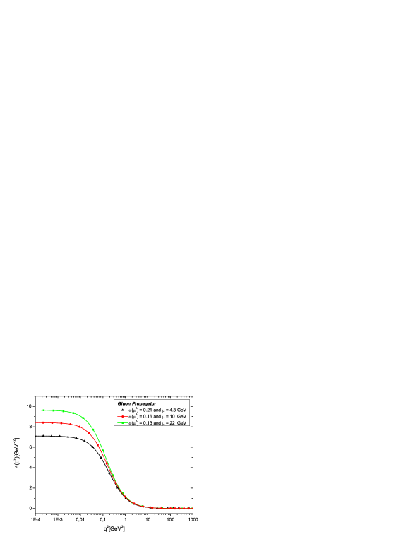
Figure 4: Numerical solutions for the gluon propagator.

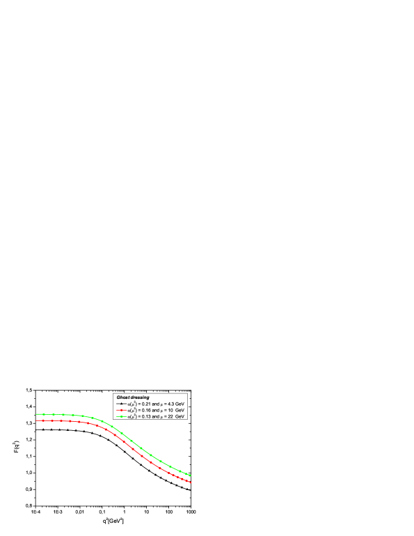
Figure 5: Numerical solutions for the ghost dressing function.

The results for $1+G(q^{2})$ and $L(q^{2})$, renormalized at the same points, are presented in Fig. 6. As we can see, the function $1+G(q^{2})$ is also IR finite exhibiting a plateau for values of $q^{2}<0.1\mbox{GeV}^{2}$. In the UV region, we instead recover the perturbative behavior (12). On the other hand, $L(q^{2})$, Fig. 7, shows a maximum in the intermediate momentum region, while, as expected, $L(0)=0$.

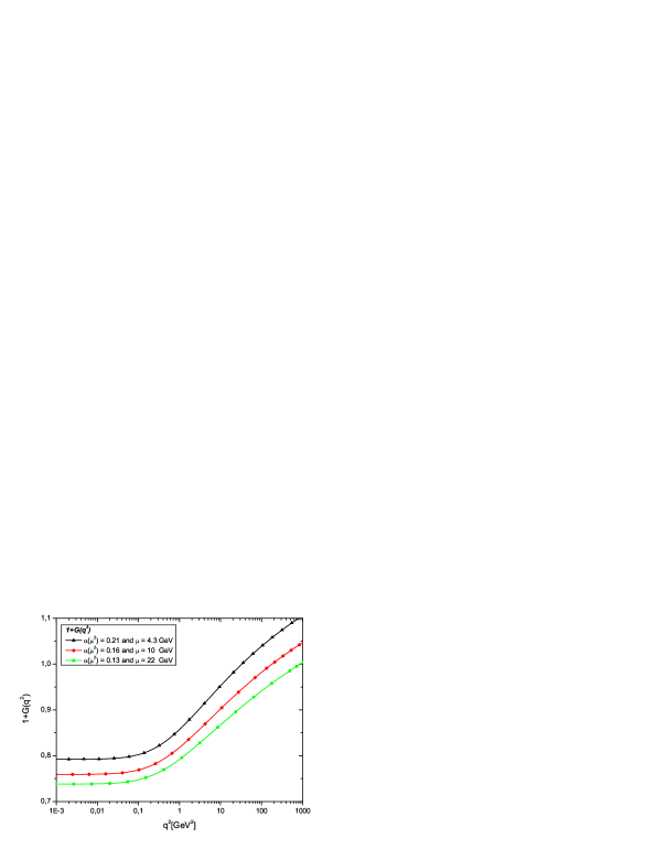
Figure 6: $1+G(q^{2})$ determined from Eq. (22).

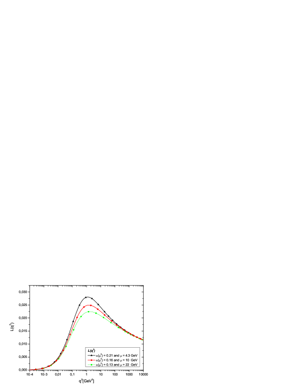
Figure 7: $L(q^{2})$ determined from Eq. (22)

With all ingredients defined, the first thing one can check is that indeed Eq. (13) gives rise to a RG-invariant combination. Using the latter definition, we can combine the different data sets for $\Delta(q^{2})$ and $[1+G(q^{2})]^{2}$ at different renormalization points, to arrive at the curves shown in Fig. 8. Indeed, we see that all curves, for different values of $\mu$, merge one into the other proving that the combination $\widehat{d}(q^{2})$ is independent of the renormalization point chosen.

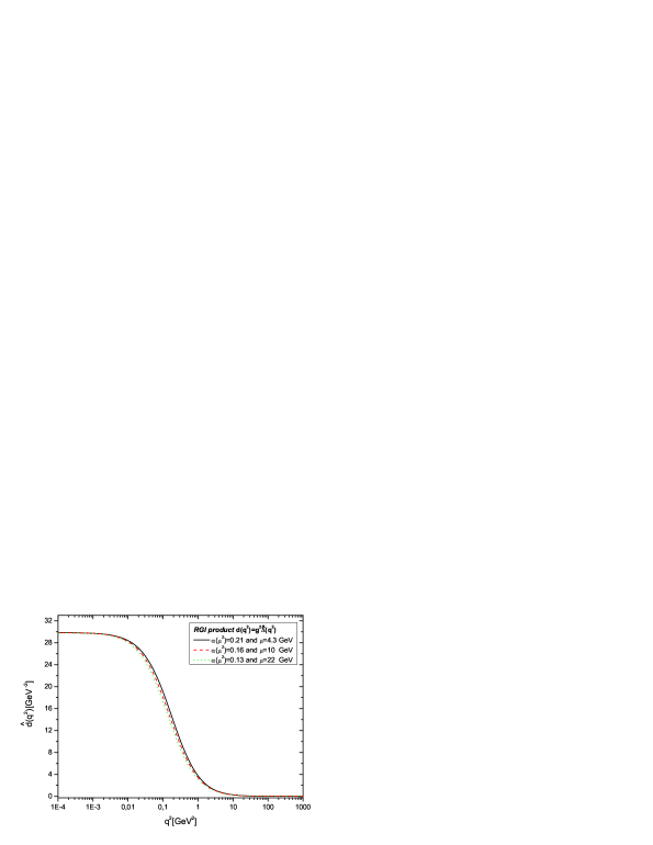
Figure 8: The $\widehat{d}(q^{2})$ obtained by combining $\Delta(q^{2})$ and $[1+G(q^{2})]^{2}$according to (13).

From the dimensionful ${\widehat{d}}(q^{2})$ we must now extract a dimensionless factor, ${\overline{g}}^{2}(q^{2})$, corresponding to the running coupling (effective charge). Given that $\Delta(q^{2})$ is IR finite (no more “scaling”!), the physically meaningful procedure is to factor out from ${\widehat{d}}(q^{2})$ a massive propagator $[q^{2}+m^{2}(q^{2})]^{-1}$,

$$\widehat{d}(q^{2})=\frac{\overline{g}^{2}(q^{2})}{q^{2}+m^{2}(q^{2})}\,,$$ (26)

where for the mass we will assume “power-law” running [11], $m^{2}(q^{2})=m^{4}_{0}/(q^{2}+m^{2}_{0})$.

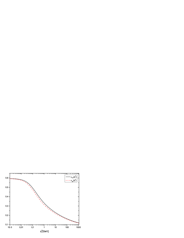
Figure 9: $\alpha_{\mathrm{gh}}(q^{2})$ vs $\alpha_{\mathrm{PT}}(q^{2})$, for $m_{0}=500\,\mbox{MeV}$.

Thus, it follows from Eq. (26), that the effective charge $\alpha_{{\scriptscriptstyle\mathrm{PT}}}=\overline{g}^{2}(q^{2})/4\pi$ is identified as being

$$4\pi\alpha_{{\scriptscriptstyle\mathrm{PT}}}(q^{2})=[q^{2}+m^{2}(q^{2})]\widehat{d}(q^{2}),$$ (27)

Finally we compare numerically the two effective charges, $\alpha_{{\scriptscriptstyle\mathrm{PT}}}(q^{2})$ and $\alpha_{\mathrm{gh}}(q^{2})$ in Fig. 9. First, we determine $\alpha_{{\scriptscriptstyle\mathrm{PT}}}(q^{2})$ obtained using (27), then we obtain $\alpha_{\mathrm{gh}}(q^{2})$ with help of (25) and the results for $1+G(q^{2})$ and $L(q^{2})$, Fig. 6 and Fig. 7.

As we can clearly see, both couplings freeze at the same finite value, exhibiting a plateau for values of $q^{2}<0.02\,\mbox{GeV}^{2}$, while in the UV both show the expected perturbative behavior. They differ only slightly in the intermediate region where the values of $L(q^{2})$ are appreciable.

5 Conclusions

In this talk we have presented a comparison between two QCD effective charge, $\alpha_{\mathrm{PT}}(q^{2})$ and $\alpha_{\mathrm{gh}}(q^{2})$, obtained from the PT and the ghost-gluon vertex, respectively.

Despite their distinct theoretical origin, due to a fundamental identity relating the various ingredients entering into their definitions, the two effective charges are almost identical in the entire range of physical momenta. In fact, the coincide exactly in the deep infrared, where they freeze at a common finite value, signaling the appearance of IR fixed point in QCD [12], also required from a variety of phenomenological studies [13].

Acknowledgments: The authors thank the organizers of LC09 for their hospitality. The research of JP is supported by the European FEDER and Spanish MICINN under grant FPA2008-02878, and the “Fundación General” of the University of Valencia.

References

- [1] A. C. Aguilar et al., Phys. Rev. D 80, 085018 (2009).
- [2] J. M. Cornwall, Phys. Rev. D 26, 1453 (1982); J. M. Cornwall and J. Papavassiliou, Phys. Rev. D 40, 3474 (1989); A. Pilaftsis, Nucl. Phys. B 487, 467 (1997); D. Binosi and J. Papavassiliou, Phys. Rev. D 66(R), 111901 (2002); Phys. Rept. 479, 1 (2009).
- [3] V. P. Nair, “Quantum field theory: A modern perspective,” New York, USA: Springer (2005) 557 p.
- [4] R. Alkofer, C. S. Fischer and F. J. Llanes-Estrada, Phys. Lett. B 611, 279 (2005).
- [5] A. C. Aguilar, D. Binosi and J. Papavassiliou, Phys. Rev. D 78, 025010 (2008).
- [6] N. J. Watson, Nucl. Phys. B 494, 388 (1997); D. Binosi and J. Papavassiliou, Nucl. Phys. Proc. Suppl. 121, 281 (2003).
- [7] L. F. Abbott, Nucl. Phys. B 185, 189 (1981).
- [8] P. A. Grassi, T. Hurth and M. Steinhauser, Annals Phys. 288, 197 (2001); D. Binosi and J. Papavassiliou, Phys. Rev. D 66(R), 025024 (2002).
- [9] T. Kugo, arXiv:hep-th/9511033; P. A. Grassi, T. Hurth and A. Quadri, Phys. Rev. D 70, 105014 (2004).
- [10] A. Cucchieri and T. Mendes, PoS LAT2007, 297 (2007); I. L. Bogolubsky, E. M. Ilgenfritz, M. Muller-Preussker and A. Sternbeck, PoS LAT2007, 290 (2007); T. Iritani, H. Suganuma and H. Iida, arXiv:0908.1311 [hep-lat]; O. Oliveira and P. J. Silva, arXiv:0910.2897 [hep-lat].
- [11] M. Lavelle, Phys. Rev. D 44, 26 (1991); A. C. Aguilar and J. Papavassiliou, Eur. Phys. J. A 35, 189 (2008); D. Dudal et al., Phys. Rev. D 78, 065047 (2008).
- [12] S. J. Brodsky and G. F. de Teramond, Phys. Lett. B 582, 211 (2004).
- [13] F. Halzen, G. I. Krein and A. A. Natale, Phys. Rev. D 47, 295 (1993); A. C. Aguilar, A. Mihara and A. A. Natale, Phys. Rev. D 65, 054011 (2002); Int. J. Mod. Phys. A 19, 249 (2004).