Optimal Decoherence Control in non-Markovian Open, Dissipative Quantum Systems

Abstract

We investigate the optimal control problem for non-Markovian open, dissipative quantum system. Optimal control using Pontryagin maximum principle is specifically derived. The influences of Ohmic reservoir with Lorentz-Drude regularization are numerically studied in a two-level system under the following three conditions: $\omega_{0}\ll\omega_{c}$, $\omega_{0}\approx\omega_{c}$ or $\omega_{0}\gg\omega_{c}$, where $\omega_{0}$ is the characteristic frequency of the quantum system of interest, and $\omega_{c}$ the cut-off frequency of Ohmic reservoir. The optimal control process shows its remarkable influences on the decoherence dynamics. The temperature is a key factor in the decoherence dynamics. We analyze the optimal decoherence control in high temperature, intermediate temperature, and low temperature reservoirs respectively. It implies that designing some engineered reservoirs with the controlled coupling and state of the environment can slow down the decoherence rate and delay the decoherence time. Moreover, we compare the non-Markovian optimal decoherence control with the Markovian one and find that with non-Markovian the engineered artificial reservoirs are better than with the Markovian approximation in controlling the open, dissipative quantum system’s decoherence.

I Introduction

The theory of open quantum systems deals with the systems that interact with their surrounding environments H.P.Breuer ; zhang ; slotine ; zanzrdi ; chuang ; Alicki ; p.zanardi . Such systems are of great interest, and these open quantum systems have been extensively studied since the origin of quantum theory J.Von. Neumann . Despite of the noticeable progresses in the theory, many fundamental difficulties still remain. One of the problem is decoherence (or loss of coherence) due to the interactions between system and environment. Recently, it received intense considerations in quantum information and quantum computation, where decoherence is regarded as a bottleneck to the construction of quantum information processor Nielsen ; Mensky ; zhang . The persistence of quantum coherence is relied on in quantum computer, quantum cryptography and quantum teleportation. And it is also fundamental in understanding the quantum world for the interpretation that the emergence of the classical world from the quantum world can be seen as a decoherence process due to the interaction between system and environment.

Various methods have been proposed to reduce this unexpected effect, such as the quantum error-correction code shor ; slotine , error-avoiding code zanzrdi ; chuang , minimal decoherence model Alicki , Bang-Bang techniques p.zanardi , quantum Zeno effect (QZE) viola and decoherence-free subspaces (DFS) elattari . Unfortunately, all of these schemes cannot suppress the unexpect effect successfully for accessorial conditions are needed. Altafini altafini pointed out that the irreversible decohering dynamics is uncontrollable under coherent control. Optimal control technique, which has been successfully studied in chemical systems rabitz ; levis ; rabitz2 and classical systems krotov , has been exploited to control the quantum decoherence Jirari ; Sugny ; zhang , where an optimal control law was designed to effectively suppress decoherence effects in Markovian open quantum systems, dynamic coupling in the spin-boson model, and time optimal control respectively. In this paper, we consider the optimal decoherence control problem in non-Markovian quantum open system.

Markovian approximation is used under the assumption that the correlation time between the systems and environments is infinitely short H.P.Breuer ; C.W.Gardiner ; zhang . For neglecting the memory effect, the Lindblad master equation has been built. However, in some cases, such as quantum Brownian motion(QBM) zurek and a two-level atom interacting with a thermal reservoir with Lorentzian spectral density Garraway , an exactly analytic description of the open quantum system dynamic is needed. Especially in high-speed communication the characteristic time scales become comparable with the reservoir correlation time, and in solid state devices memory effects are typically non negligible. So it is necessary to extensively study the non-Markovian master equation. We briefly compare the non-Markovian dynamics (non-Markovian master equation) with Markovian process (Markovian master equation) in Appendix A. For details one can refer to Gardiner’s book C.W.Gardiner or/and Breuer’s H.P.Breuer .

In this paper the focus will be on the optimal decoherence control of non-Markovian quantum system, particularly the simplest system possible, a two-level system governed by the time-convolutionless (TCL) equation. We determine control fields which minimize the cost functional suppressing the decoherence process by applying the Pontryagin maximum principle (PMP) in Ohmic reservoir with Lorentz-Drude regularization in the following three conditions: $\omega_{0}\ll\omega_{c}$, $\omega_{0}\approx\omega_{c}$, $\omega_{0}\gg\omega_{c}$, where $\omega_{0}$ is the characteristic frequency of the quantum system of interest and $\omega_{c}$ the cut-off frequency of Ohmic reservoir. Thus, $\omega_{c}\ll\omega_{0}$ implies that the spectrum of the reservoir does not completely overlap with the frequency of the system oscillator and $\omega_{0}\gg\omega_{c}$ implies the converse case. With this it is possible to engineer different types of artificial reservoir, and couple them to the system in a controlled way. We also compare our results with no-control system evolution and the optimal control of the open system with Markovian approximation. The main result of the paper is that decoherence phenomenon can be successfully suppressed in the $\omega_{0}\ll\omega_{c}$ case. Then this explores the coupling of the system to engineered reservoirs Myatt ; Turchette , in which the coupling and state of the environment are controllable. This may pave a newly way to the realization of the first basic elements of quantum computers.

The paper is organized as follows. We first introduce quantum decoherence and the quantum master equation for driven open quantum systems. In Sec. III we formulate the optimal control formalism and deduced PMP with a minimum cost functional. Moreover, we consider the non-Markovian two-level optimal control problem. In Sec. IV, we numerically analyze the optimal control of decoherence to the two-level system, and analyze the difference between Markovian optimal control and non-Markovian optimal control from both the system time evolution and the power spectrum. Conclusions and prospective views are given in Sec.V.

II Modeling the quantum decoherence control system

Consider a quantum system $S$ embedded in a dissipative environment $B$ and interacting with a time-dependent classical external field, i.e., the control field. The total Hamiltonian has the general form

$$\begin{array}[]{rcl}H_{tot}&=&H_{0}+H_{B}+H_{int}\\ &=&H_{S}+H_{C}(t)+H_{B}+H_{int},\end{array}$$ (1)

where $H_{S}$ is the Hamiltonian of the system, $H_{C}(t)$ the Hamiltonian of the control field, and $H_{B}$ the bath and $H_{int}$ their interaction that is responsible for decoherence. The operators $H_{S}$ and $H_{B}$ act on $\mathcal{H}_{S}$ and $\mathcal{H}_{B}$, respectively. The operator $H_{C}(t)$ contains a time-dependent external field to adjust the quantum evolution of the system. One of the central goals of the theoretical treatment is then the analysis of the dynamical behavior of the populations and coherences, which are given by the elements of the reduced density matrix, defined as

$$\begin{split}\rho_{S}(t)=tr_{B}[\rho_{tot}(t)],\end{split}$$ (2)

where $\rho_{tot}$ is the total density matrix for both the system and the environment, $tr_{B}$ the partial trace taken over the environment. The driven model consists of a $N$-level system interacting with a thermal bath in the presence of external control field zhang ; zhang2 , and the Hamiltonian is

$$\begin{split}H_{C}(t)=\sum_{i}u_{i}(t)H_{i}\end{split}$$ (3)

$H_{i}$ is the control Hamiltonian adjusted by the control parameters $u_{i}(t)$, and $u_{i}(t)$ represents the control field. The Hamiltonian of the environment is assumed to be composed of harmonic oscillators with natural frequencies $\omega_{i}$ and masses $m_{i}$,

$$\begin{split}H_{B}=\sum_{i=1}^{N}(\frac{p_{i}^{2}}{2m_{i}}+\frac{m_{i}}{2}x_{i}^{2}\omega_{i}^{2}),\end{split}$$ (4)

where $(x_{1},x_{2},\cdots,x_{N},p_{1},p_{2},\cdots,p_{N})$ are the coordinates and their conjugate momenta, and the Planck constant $\hbar$ is assigned to be $1$. The interaction Hamiltonian between the system $S$ and the environment $B$ is assumed to be bilinear H.P.Breuer ,

$$\begin{split}H_{int}=\alpha\sum_{n}A_{n}\otimes B_{n}.\end{split}$$ (5)

The interaction Hamiltonian in the interaction picture therefore takes the form

$$\begin{array}[]{rcl}H_{int}(t)&=&e^{i(H_{S}+H_{B})t}H_{int}e^{-i(H_{S}+H_{B})t}\\ &=&\alpha\sum_{n}A_{n}(t)\otimes B_{n}(t),\end{array}$$ (6)

where

$$\begin{array}[]{rcl}A_{n}(t)&=&e^{iH_{S}t}A_{n}e^{-iH_{S}t},\\ B_{n}(t)&=&e^{iH_{B}t}B_{n}e^{-iH_{B}t}.\end{array}$$

The effect of the environment on the dynamics of the system can be seen as a interplay between the dissipation and fluctuation phenomena. And it is the general environment that makes the quantum system loss of coherence (decoherence). In general the decoherence can be demonstrated as the interaction between the system and environment. Then the reduced density matrix of the system can evolve into the form

$$\begin{split}\rho_{T}\simeq\sum_{n}|c_{n}|^{2}|a_{n}\rangle\langle a_{n}|\end{split}$$ (7)

which describes a statistical mixture of noninterfering states. Thus, a commonly proposed way to analyze decoherence is by examining how the nondiagonal elements of the reduced density matrix evolve under the master equation.

In the present work, we shall concentrate on optimal control of the decoherence effect in open quantum system. The kinetic equation of strong coupling non-Markovian quantum system is the following exact time-convolutionless (TCL) form of the master equation,

$$\begin{split}\frac{d}{dt}\mathcal{P}\rho(t)=\sum_{i}u_{i}\tilde{\mathcal{K}}_{i}(t)\mathcal{P}\rho(t)+\mathcal{K}(t)\mathcal{P}\rho(t)+\mathcal{I}(t)\mathcal{Q}\rho(t_{0}),\end{split}$$ (8)

with the time-local generator, called the TCL generator

$$\begin{split}\tilde{\mathcal{K}}_{i}(t)=e^{iH_{S}t}H_{i}e^{-iH_{S}t},~{}~{}~{}~{}\mathcal{K}(t)=\alpha\mathcal{P}\mathcal{L}(t)[1-\Sigma(t)]^{-1}\mathcal{P},\end{split}$$ (9)

and the inhomogeneity

$$\begin{split}\mathcal{I}(t)=\alpha\mathcal{P}\mathcal{L}(t)[1-\Sigma(t)]^{-1}g(t,t_{0})\mathcal{Q},\end{split}$$ (10)

where $\Sigma(t)$ is the superoperator

$$\Sigma(t)=\alpha\int_{t_{0}}^{t}ds\mathcal{G}(t,s)\mathcal{Q}\mathcal{L}(s)\mathcal{P}G(t,s).$$

For detail one see Appendix A and/or H.P.Breuer

In order to facilitate the calculations, we will convert the differential equation (8) from the complex density matrix representation into the so-called coherent vector representation Blum ; altafini ; zhang . Firstly, we choose an orthonormal basis of $N\times N$ matrices $\{(I,\Omega_{j})\}_{j=1,2,\cdots,N^{2}-1}$ with respect to the inner product $\langle X,Y\rangle=tr(X^{{\dagger}}Y)$, where $I$ is the N-dimensional identity matrix and $\Omega_{j}$ are $N\times N$ Hermitian traceless matrices. In particular, the Hermitian density matrix $\rho$ can be represented as $\rho=\frac{1}{N}I+\sum_{i}x_{i}\cdot\Omega_{i}$, where $\vec{x}=(x_{1},x_{2},\cdots x_{N^{2}-1})^{T}$ is a real $(N^{2}-1)$ dimensional vector, called the coherent vector of $\rho$. This is the well-known Bloch vector representation of quantum systems. Thus the master equation (8) can be rewritten as a differential equation of the coherent vector:

$$\begin{array}[]{rcl}\dot{x}(t)&=&O_{0}x(t)+\sum_{i=1}^{k}u_{i}(t)O_{i}x(t)+L_{1}(t)x(t)+L_{2}(t),\\ \end{array}$$ (11)

with the initial condition,

$$x(t_{0})=x_{0}$$

where $O_{0},O_{i}\in\text{so}(N^{2}-1)$ are the adjoint representation matrices of $-iH_{0},-iH_{i}$ respectively, and $x_{0}$ is the coherence vector of $\rho_{0}$, and the term $L_{1}(t)x(t)$ represents the decoherence process, $k$ is the number of control fields, $\sum_{i}^{k}u_{i}H_{i}$ adjusts the quantum evolution such that the coherence is conserved.

III quantum optimal control problem

III.1 General Formalism

As well known, the evolution of the state variable $x(t)$ governed by the master equation (11) depends not only on the initial state $x_{0}$ but also on the choice of the time-dependent control variable $u(t)$. Some earlier works to these control problem are listed in the reference Thorwart ; Grifoni ; Shao . Especially, the exact result was considered of the quantum two-state dynamics driven by stationary non-Markovian discrete noise in Goychuk . In this section, we are going to suppress the unexpected effect of decoherence by optimal control technique that wants to force the system evolving along some prescribed cohering trajectories. The target state chosen is the free evolution of the closed system:

$$\begin{split}\dot{\rho}_{T}(t)=-i[H_{0},\rho_{T}(t)],\end{split}$$ (12)

which is equivalent to $x^{0}(t)=e^{O_{0}(t-t_{0})}x_{0}$. The cost functional is

$$\begin{split}J[u(t)]=\Psi[x(t_{f}),x^{0}(t_{f})]+\int_{t_{o}}^{t_{f}}\Theta(x(t),x^{0}(t_{f}),u(t))dt,\end{split}$$ (13)

where the functional $\Psi[x(t_{f}),x^{0}(t_{f})]$ represents distance between the system and objects at final time and the functional $\int_{t_{o}}^{t_{f}}\Theta(x(t),x^{0}(t_{f}),u(t))$ accounts for the transient response with $\Theta(x(t),x^{0}(t_{f}),u(t))\geq 0$.

The optimal control problem considered in this paper is to minimize the cost functional $J[u(t)]$ with some dynamical constraints. That is, our problem is

$$\begin{array}[]{rcl}\min_{u\in\mathcal{U}_{[t_{0},t_{f}]}}J[u(t)]&=&\Psi[x(t_{f}),x^{0}(t_{f})]+\int_{t_{o}}^{t_{f}}\Theta(t)dt,\\ \dot{x}(t)&=&O_{0}x(t)+\sum_{i=1}^{k}u_{i}(t)O_{i}x(t)\\ &+&L_{1}(t)x(t)+L_{2}(t),\\ x(t_{0})&=&x_{0},~{}t\in[t_{0},t_{f}],\end{array}$$ (14)

where $\mathscr{U}_{[t_{0},t_{f}]}=\{u(\cdot):[t_{0},t_{f}]\longrightarrow\mathbb{R}^{k}\}$ and $u(\cdot)$ piecewise continuous.

Using the Pontryagin’s maximum principle krotov , the optimal solution to this problem is characterized by the following Hamilton-Jacobi-Bellman(HJB) Equation

$$\begin{cases}\frac{\partial J}{\partial t}+min_{u\in\mathscr{U}_{[t_{0},t_{f}]}}\{O_{0}x(t)+\sum_{i=1}^{k}u_{i}(t)O_{i}x(t)+L_{1}(t)x(t)+L_{2}(t)+\Theta(x(t),x^{0}(t_{f}),u(t))\}=0,\\ J(x(t_{f}),t_{f})=\Psi[x(t_{f})].\end{cases}$$ (15)

In general, it is usually difficult to obtain the analytic solution. Nevertheless, one can always have numerical solution. To illustrate this method and give more insight, we will consider this problem for the non-Markovian two-level system in the following.

III.2 Optimal Control of non-Markovian Two-Level System

In this subsection we consider the decoherence of two-level system whose controlled Hamiltonian is

$$H_{0}=\frac{1}{2}\{\omega_{0}\sigma_{z}+u_{x}(t)\sigma_{x}+u_{y}(t)\sigma_{y}\},$$ (16)

where $\sigma_{k}$ with $k=x,y,z$ are the Pauli matrices; $\omega_{0}$ is the transition frequency of the two-level system, and $u(t)$ is the modulation by the time-dependent external control field. In fact, the free Hamiltonian is $H_{S}=\frac{1}{2}\omega\sigma_{z}$. Then the control Hamiltonian can be described by $\sigma_{x},\sigma_{y}$ according to Cartan decomposition of the Lie algebra $\text{su}(2)$, which was discussed by Zhang et. al in details zhang2 . This is the standard model for atom-field interaction scully ; meystre ; Anastopoulos ; Shresta .

In our two-level system the assumed bilinear interaction between the system $S$ and the environment $B$ can be written as

$$H_{int}=\alpha\left(\sigma_{+}\otimes B+\sigma_{-}\otimes B^{{\dagger}}\right)~{}~{}~{}\text{with}~{}~{}B=\sum_{i}k_{i}a_{i},$$ (17)

where $\sigma_{\pm}=(\sigma_{x}\pm i\sigma_{y})/2$, the raising and lowering operator respectively, $k_{i}$ is the coupling constant between the spin coordinate and the $i$th environment oscillator, and $a_{i}$ is the annihilation operator of the $i$th harmonic oscillators of the environment. The coupling constants enter the spectral density function $J(\omega)$ of the environment defined by

$$J(\omega)=\frac{\pi}{2}\sum_{i}\frac{k_{i}}{m_{i}\omega_{i}}\delta(\omega-\omega_{i})$$ (18)

and the index $i$ labels the different field models of the reservoir with frequencies $\omega_{i}$. In the continuum limit the spectral density has the form

$$\begin{split}J(\omega)=\eta\omega(\frac{\omega}{\omega_{c}})^{n-1}\exp(-\frac{\omega}{\omega_{c}}),\end{split}$$ (19)

where $\omega_{c}$ is a cutoff frequency, and $\eta$ a dimensionless coupling constant. The environment is classified as Ohmic, sub-Ohmic, and sup-Ohmic according to $n=1$, $0<n<1$, and $n>1$, respectively An ; Leggett ; weiss .

In this case, the open quantum system can be written as follows H.P.Breuer ; Maniscalco ; Maniscalco2

$$\begin{array}[]{rcl}\dot{\rho}_{S}=-\frac{i}{2}\omega_{0}[\sigma_{z},\rho_{S}]-\frac{i}{2}u_{x}(t)[\sigma_{x},\rho_{S}]-\frac{i}{2}u_{y}(t)[\sigma_{y},\rho_{S}]\\ +\frac{\Delta(t)+\gamma(t)}{2}\{2\sigma_{-}\rho_{S}\sigma_{+}-\sigma_{+}\sigma_{-}\rho_{S}-\rho_{S}\sigma_{+}\sigma_{-}\}\\ +\frac{\Delta(t)-\gamma(t)}{2}\{2\sigma_{+}\rho_{S}\sigma_{-}-\sigma_{-}\sigma_{+}\rho_{S}-\rho_{S}\sigma_{-}\sigma_{+}\}.\end{array}$$ (20)

For convenience we map the density matrix of the two-level system onto the Bloch vector $x(t)=(x_{1}(t),x_{2}(t),x_{3}(t))^{T}\in\mathbb{R}^{3}$ defined by $x(t)=Tr[\sigma\rho(t)]$, which implies that

$$\begin{array}[]{rcl}x_{1}(t)&\equiv&\rho_{01}(t)+\rho_{10}(t),\\ x_{2}(t)&\equiv&i(\rho_{01}(t)-\rho_{10}(t)),\\ x_{3}(t)&\equiv&\rho_{00}(t)-\rho_{11}(t).\end{array}$$ (21)

Then the explicit equations of motion for the components of the Bloch vector read

$$\left\{\begin{array}[]{rcl}\dot{x_{1}}(t)&=&-\Delta(t)x_{1}(t)-\omega_{0}x_{2}(t)+x_{3}(t)u_{y}(t),\\ \dot{x_{2}}(t)&=&\omega_{0}x_{1}(t)-\Delta(t)x_{2}(t)-x_{3}(t)u_{x}(t),\\ \dot{x_{3}}(t)&=&-2\Delta(t)x_{3}(t)-2\gamma(t)+x_{2}(t)u_{x}(t)-x_{1}(t)u_{y}(t),\end{array}\right.$$ (22)

where the expressions for the relevant time dependent coefficients, up to the second order in the system-reservoir coupling constant, are given by Maniscalco ; H.P.Breuer

$$\begin{array}[]{rcl}\Delta(t)&=&\int_{0}^{t}d\tau k(\tau)\cos(\omega_{0}\tau)\\ \gamma(t)&=&\int_{0}^{t}d\tau\mu(\tau)\sin(\omega_{0}\tau)\end{array}$$ (23)

with

$$\begin{array}[]{rcl}k(\tau)&=&2\int_{0}^{\infty}d\omega J(\omega)\coth[\hbar\omega/2k_{B}T]\cos(\omega\tau),\\ \mu(\tau)&=&2\int_{0}^{\infty}d\omega J(\omega)\sin(\omega\tau),\end{array}$$ (24)

being the noise and the dissipation kernels, respectively. The equation (22) can be written compactly as

$$\begin{split}\dot{x}(t)=A(t)x(t)+B(t),\end{split}$$ (25)

where

$$A(t)=\left(\begin{array}[]{ccc}-\Delta(t)&-\omega_{0}&u_{y}(t)\\ \omega_{0}&-\Delta(t)&-u_{x}(t)\\ -u_{y}(t)&u_{x}(t)&-2\Delta(t)\end{array}\right)$$

and

$$B(t)=\left(\begin{array}[]{ccc}0\\ 0\\ -2\gamma(t)\end{array}\right).$$

Let the Ohmic spectral density with a Lorentz-Drude cutoff function,

$$\begin{split}J(\omega)=\frac{2\gamma_{0}}{\pi}\omega\frac{\omega_{c}^{2}}{\omega_{c}^{2}+\omega^{2}},\end{split}$$ (26)

where $\gamma_{0}$ is the frequency-independent damping constant and usually assumed to be $1$. $\omega$ is the frequency of the bath, and $\omega_{c}$ is the high-frequency cutoff. For this type of spectral density the bath correlations can be determined analytically as

$$\begin{split}k(\tau)=4k_{B}T{\omega_{c}}^{2}\sum_{n=-\infty}^{+\infty}\frac{\omega_{c}e^{-{\omega_{c}}|\tau|}-|\nu_{n}|e^{-|\nu_{n}||\tau|}}{\omega_{c}^{2}-\nu_{n}^{2}}\end{split}$$ (27)

where $\nu_{n}=2\pi nk_{B}T$ and

$$\begin{split}\mu(\tau)=2\hbar\omega_{c}^{2}e^{-\omega_{c}|\tau|}sign~{}\tau.\end{split}$$ (28)

Then the analytic expression for the dissipation coefficient $\gamma(t)$ appearing in the equation (23) is

$$\begin{split}\gamma(t)=\frac{\alpha^{2}\omega_{0}r^{2}}{1+r^{2}}[1-e^{-r\omega_{0}t}\cos(\omega_{0}t)-re^{-r\omega_{0}t}\sin(\omega_{0}t)],\end{split}$$ (29)

and the closed analytic expression for $\Delta(t)$ is Maniscalco2

$$\begin{array}[]{rcl}\Delta(t)&=&\alpha^{2}\omega_{0}\frac{r^{2}}{1+r^{2}}\{\coth(\pi r_{0})-\cot(\pi r_{c})e^{-\omega_{c}t}[r\cos(\omega_{0}t)-\sin(\omega_{0}t)]+\frac{1}{\pi r_{0}}\cos(\omega_{0}t)[\bar{F}(-r_{c},t)\\ &&+\bar{F}(r_{c},t)-\bar{F}(ir_{0},t)-\bar{F}(-ir_{0},t)]-\frac{1}{\pi}\sin(\omega_{0}t)[\frac{e^{-\nu_{1}t}}{2r_{0}(1+r_{0}^{2})}[(r_{0}-i)\bar{G}(-r_{0},t)\\ &&+(r_{0}+i)\bar{G}(r_{0},t)]+\frac{1}{2r_{c}}[\bar{F}(-r_{c},t)-\bar{F}(r_{c},t)]]\},\end{array}$$ (30)

where $r_{0}=\omega_{0}/2\pi k_{B}T$, $r_{c}=\omega_{c}/2\pi k_{B}T$, $r=\omega_{c}/\omega_{0}$, and

$$\begin{split}\bar{F}(x,t)\equiv_{2}F_{1}(x,1,1+x,e^{-\nu_{1}t}),\end{split}$$ (31)

$$\begin{split}\bar{G}(x,t)\equiv_{2}F_{1}(2,1+x,2+x,e^{-\nu_{1}t}).\end{split}$$ (32)

${}_{2}F_{1}(a,b,c,z)$ is the hypergeometric function and takes the form

$${}_{2}F_{1}(a,b,c,z) = 1+\frac{ab}{1!c}z+\frac{a(a+1)b(b+1)}{2!c(c+1)z^{2}}z^{2}+\cdots$$

$$= \sum_{n=0}^{\infty}\frac{(a)_{n}(b)_{n}}{(c)_{n}}\frac{z^{n}}{n!},$$

where $(a)_{n}$ is a Pochhammer symbol. Under the high temperature limit, we have

$$\begin{split}\Delta(t)=2\alpha^{2}\kappa T\frac{r^{2}}{1+r^{2}}\{1-e^{-r\omega_{0}t}[\cos(\omega_{0}t)-\frac{1}{r}\sin(\omega_{0}t)]\}.\end{split}$$ (33)

In the following we consider the optimal control formalism of our two-level system. For simplicity we define the cost functional as:

$$\begin{split}J[u(t)]=\int_{t_{0}}^{t_{f}}[(x(t)-x^{0}(t))^{2}+\theta u^{T}(t)u(t)]dt\end{split}$$ (34)

where $\theta>0$ is a weighting factor used to achieve a balance between the tracking precision and the control constraints. The corresponding Hamiltonian function is

$$\mathcal{H}(x(t),u(t),\lambda(t),t) = [(x(t)-x^{0}(t))^{2}+\theta u^{T}(t)u(t)]+\lambda(t)^{T}[A(t)x(t)+B(t)]$$

$$= [(x_{1}(t)-x_{1}^{0}(t))^{2}+(x_{2}(t)-x_{2}^{0}(t))^{2}+(x_{3}(t)-x_{3}^{0}(t))^{2}+\theta(u_{1}^{2}(t)+u_{2}^{2}(t))]$$

$$+\lambda_{1}(t)[-\Delta(t)x_{1}(t)-\omega_{0}x_{2}(t)+x_{3}(t)u_{y}(t)]+\lambda_{2}(t)[\omega_{0}x_{1}(t)-\Delta(t)x_{2}(t)$$

$$-x_{3}(t)u_{x}(t)]+\lambda_{3}(t)[-2\Delta(t)x_{3}(t)-2\gamma(t)+x_{2}(t)u_{x}(t)-x_{1}(t)u_{y}(t)],$$

where $\lambda(t)=(\lambda_{1}(t),\lambda_{2}(t),\lambda_{3}(t))^{T}$ is the so-called Lagrange multiplier and $x^{0}(t)=(x^{0}_{1}(t),x^{0}_{2}(t),x^{0}_{2}(t))$ is the target trajectory defined by $\dot{\rho}=-\frac{i}{2}[H_{0},\rho]$. It is easy to see that $x^{0}(t)=(x^{0}_{1}\cos\omega t-x^{0}_{2}\sin\omega t,x^{0}_{1}\sin\omega t+x^{0}_{2}\cos\omega,x^{0}_{3})$. The optimal solution can be solved by the following differential equation with two-sided boundary values,

$$\begin{cases}\dot{x}^{*}(t)=\frac{\partial\mathcal{H}}{\partial\lambda}=A(t)x(t)+B(t)\\ \dot{\lambda}(t)=-\frac{\partial\mathcal{H}}{\partial x}=-2[x(t)-x^{0}(t)]-A(t)^{T}\lambda(t)\\ x^{*}(0)=x_{0}\\ \lambda(t_{f})=0\end{cases}$$ (35)

together with

$$\begin{cases}\frac{\partial\mathcal{H}}{\partial u}|_{*}=\frac{\partial\mathcal{H}(x^{*}(t),u^{*}(t),\lambda(t),t)}{\partial u}=0,\\ \frac{\partial^{2}\mathcal{H}}{\partial u^{2}}|_{*}=\frac{\partial^{2}\mathcal{H}(x^{*}(t),u^{*}(t),\lambda(t),t)}{\partial u^{2}}\leq 0,\end{cases}$$ (36)

which implies that

$$\begin{cases}u_{x}(t)=\frac{1}{2\theta}\{\lambda_{2}x_{3}-\lambda_{3}x_{2}\},\\ u_{y}(t)=\frac{1}{2\theta}\{\lambda_{3}x_{1}-\lambda_{1}x_{3}\}.\end{cases}$$ (37)

The minimum principle requires the solution of the complicated nonlinear equations. When there is one and only one solution $\{x(t),~{}\lambda(t)\}$ it is the required optimal solution krotov . In general, it is difficult to obtain the analytic solution, if possible existence, to the above optimal control problem. So numerical demonstration to this problem will be considered in the next section.

IV numerical demonstration and discussions

In this section, we use the formalism of the preceding section to determine the optimal control of the decoherence. Though the spin-bath models of real systems are expected to be more complicated than the two-level Hamiltonians considered here, we study the system in various aspects to understand the effect of this simple system on the decoherence control.

In our simulations, the system parameters are chosen as following, $x(0)=(\frac{\sqrt{3}}{2},\frac{-\sqrt{2}}{4},\frac{-\sqrt{2}}{4})$, strong coupling constant $\alpha^{2}=0.01$, weighting factor $\theta=1$, $\omega_{0}=1$ as the norm unit. Moreover, we regard the temperature as a key factor in decoherence process. For high temperature $k_{B}T=300\omega_{0}$, intermediate temperature $k_{B}T=3\omega_{0}$, and low temperature $k_{B}T=0.3\omega_{0}$. Another reservoir parameter playing a key role in the dynamics of the system is the ratio $r=\omega_{c}/\omega_{0}$ between the reservoir cutoff frequency $\omega_{c}$ and the system oscillator frequency $\omega_{0}$. As we will see in this section, by varying these two parameters $k_{B}T$ and $r=\omega_{c}/\omega_{0}$, both the time evolution and the optimal control of the open system vary prominently from Markovian to non-Markovian.

IV.1 High temperature reservoir

For high reservoir temperature, diffusion coefficient $\Delta(t)$ (30) has the approximation form (33), which plays a dominant role since $\Delta(t)\gg\gamma(t)$. Note that, for time $t$ large enough, the coefficients $\Delta(t)$ and $\gamma(t)$ can be approximated by their Markovian stationary values $\Delta_{M}=\Delta(t\rightarrow\infty)$ and $\gamma_{M}=\gamma(t\rightarrow\infty)$. From eqs.(29) and (30) we have

$$\gamma_{M}=\frac{\alpha^{2}\omega_{0}r^{2}}{1+r^{2}},$$ (38)

and

$$\Delta_{M}=\alpha^{2}\omega_{0}\frac{r^{2}}{1+r^{2}}\coth(\pi r_{0}).$$ (39)

Then, under high temperature, noting

$$\coth(\pi r_{0})\simeq 1+\frac{1}{\pi r_{0}}\simeq\frac{2kT}{\omega_{0}},$$

$$\Delta_{M}^{HT}=2\alpha^{2}kT\frac{r^{2}}{1+r^{2}}.$$ (40)

Inserting Eqs.(38) and (40) into Eqs.(35) one can easily get the Markovian optimal decoherence control.

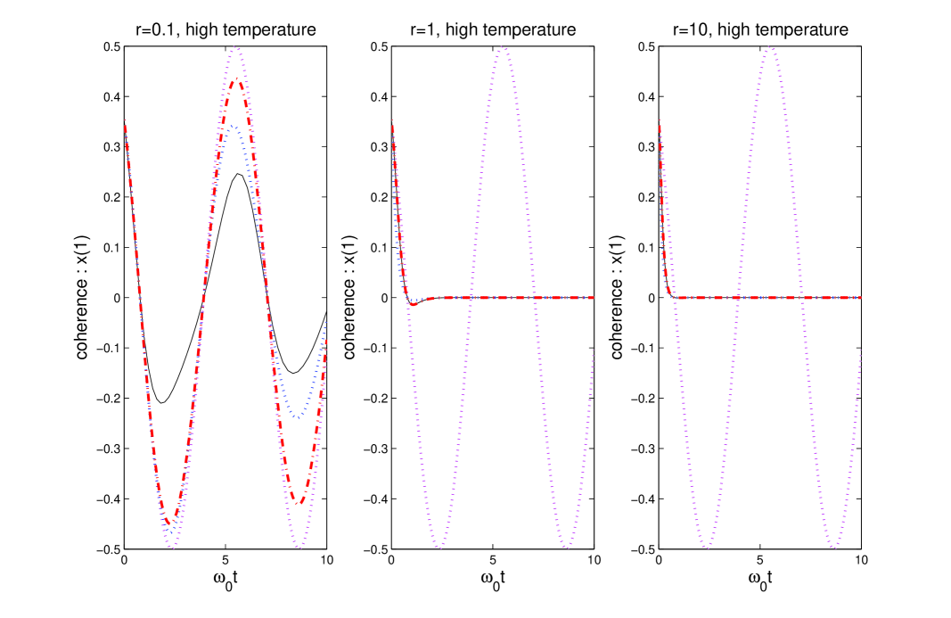
Figure 1: (Color online)Surviving coherence in off-diagonal matrix elements vs time $t$ [Eq.35] under high temperature environment, without control action(black solid line), Markovian optimal control(blue dashed line), non-Markovian optimal control(red dotted line), and target trajectory(crimson dash-dotted line) at $r=0.1$, $r=1$, $r=10$ respectively.

Figure 1 shows optimal control of decoherence for $r\ll 1,~{}~{}r=1$,  and $r\gg 1$ in high temperature reservoir. All of these contain solid line for free evolution, dashed line for Markovian optimal control, dotted line for non-Markovian optimal control, and dash-dotted line for target trajectory. We can see clearly that the decoherence can be controlled perfectly in $r\ll 1$ reservoir. From Figure 2 we can see that the decoherence time $\tau_{D}$ can be delayed for a long time and its amplitude amplified heavily with the non-Markovian control. On the other hand, Figure 3 shows that the non-Markovian control field is changed more rapidly than the Markovian control field and the frequency of non-Markovian is more plenty than the Markovian, which helps to understand that the non-Markovian case is done better than the Markovian case and implies that it is necessary to consider the non-Markovian case.

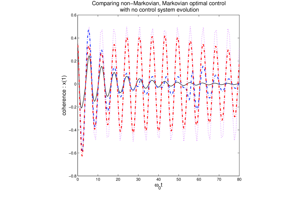
Figure 2: (Color online)Comparing Markovian optimal control, non-Markovian optimal control with no control under high temperature environment, without control action(black solid line), Markovian optimal control(blue dashed line), non-Markovian optimal control(red dotted line), and target trajectory(crimson dash-dotted line) at $r=0.1$.

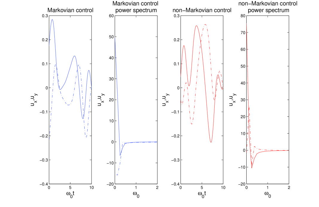
Figure 3: (Color online)Comparing Markovian optimal control with non-Markovian one in r=0.1 high temperture reservoir. Markovian optimal control $u_{x}$(blue solid line) $u_{y}$(blue dash-dotted line) , non-Markovian optimal control $u_{x}$(red solid line) $u_{y}$ (red dash-dotted line).

From Figure 1 we can also see that either Markovian or non-Markovian optimal control cannot do well when $r=1$ or $r=10$. As we discussed before, diffusion is always dominant under the high temperature. In the case $r\ll 1$, $\Delta(t)>0$ is always true Maniscalco2 . However, Maniscalco, et. al. Maniscalco2 showed that if $r>0.27$ the diffusion coefficient $\Delta(t)<0$, and the system becomes non-Lindblad. It implies that the environment induced fluctuations will be large enough. So our control field is negligible when comparing with the high-frequency harmonic oscillators of the reservoir.

IV.2 Lower temperature reservoir

As decreasing temperature, the amplitude of $\Delta(t)$ becomes smaller and smaller and $\gamma(t)$ becomes larger and larger, which is not negligible anymore. There exists a time which relate to both the temperature and the ratio such that after the time the combination of dissipation and diffusion coefficient $\Delta(t)-\gamma(t)<0$, which changes the properties of the control system (35).

Figure 4 shows the non-Markovian optimal control and Figure 5 their power spectrum for intermediate temperature, and Figure 6 and Figure 7 for low temperature. At intermediate temperature the non-Markovian optimal control plays little role especially in Figure 4(b)and Figure 4(c). Note that in Figure 4(a) and 6(a) the free evolution is with little decoherence. We note that the optimal control does well at low temperature in Figure 6. In Figure 6, both Markovian and non-Markovian play an important role in controlling the decoherence in both $r=1$ and $r=10$. They can make the quantum coherence persistence for a long time.

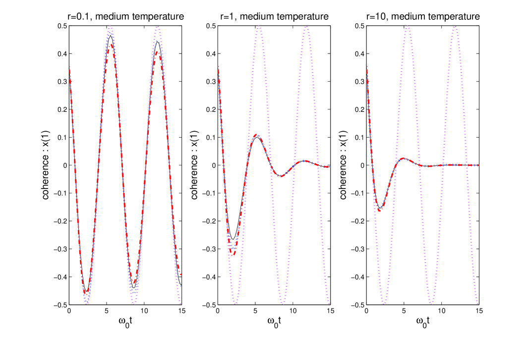
Figure 4: (Color online)Surviving coherence in off-diagonal matrix elements vs time $t$ [Eq.35] under medium temperature environment, without control action(black solid line), Markovian optimal control(blue dashed line), non-Markovian optimal control(red dotted line), and target trajectory(crimson dash-dotted line) at $r=0.1$, $r=1$, $r=10$ respectively.

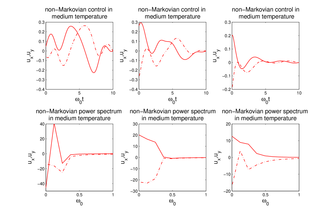
Figure 5: (Color online)non-Markovian optimal controls and their power spectrum in medium temperature reservoir for $r=0.1$, $r=1$, and $r=10$ respectively. Non-Markovian optimal control $u_{x}$(red solid line) $u_{y}$(red dash-dotted line).

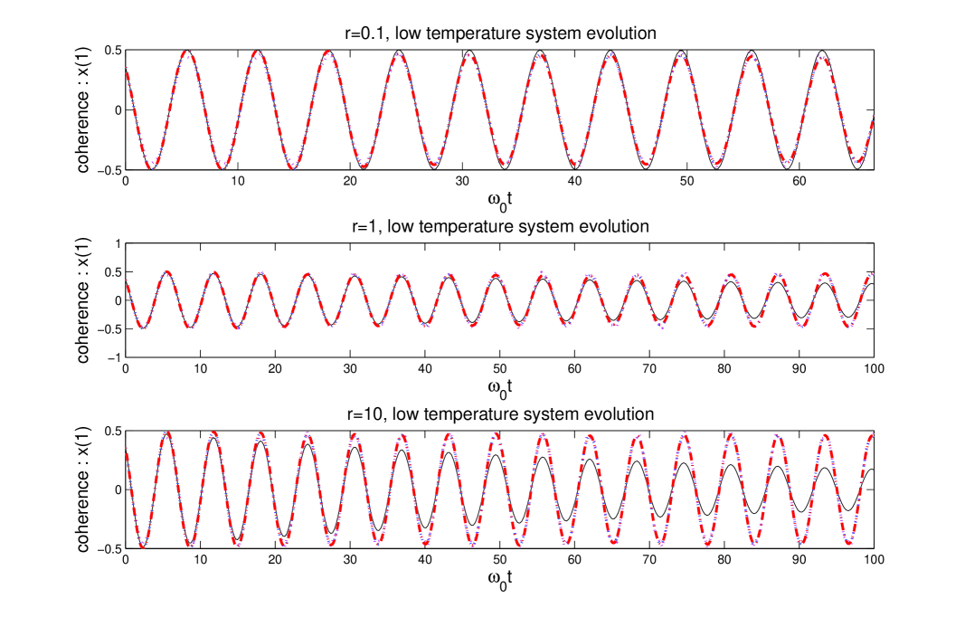
Figure 6: (Color online)Surviving coherence in off-diagonal matrix elements vs time $t$ [Eq.35] under low temperature environment, without control action(black solid line), Markovian optimal control(blue dashed line), non-Markovian optimal control(red dotted line), and target trajectory(crimson dash-dotted line) at $r=0.1$, $r=1$, $r=10$ respectively.

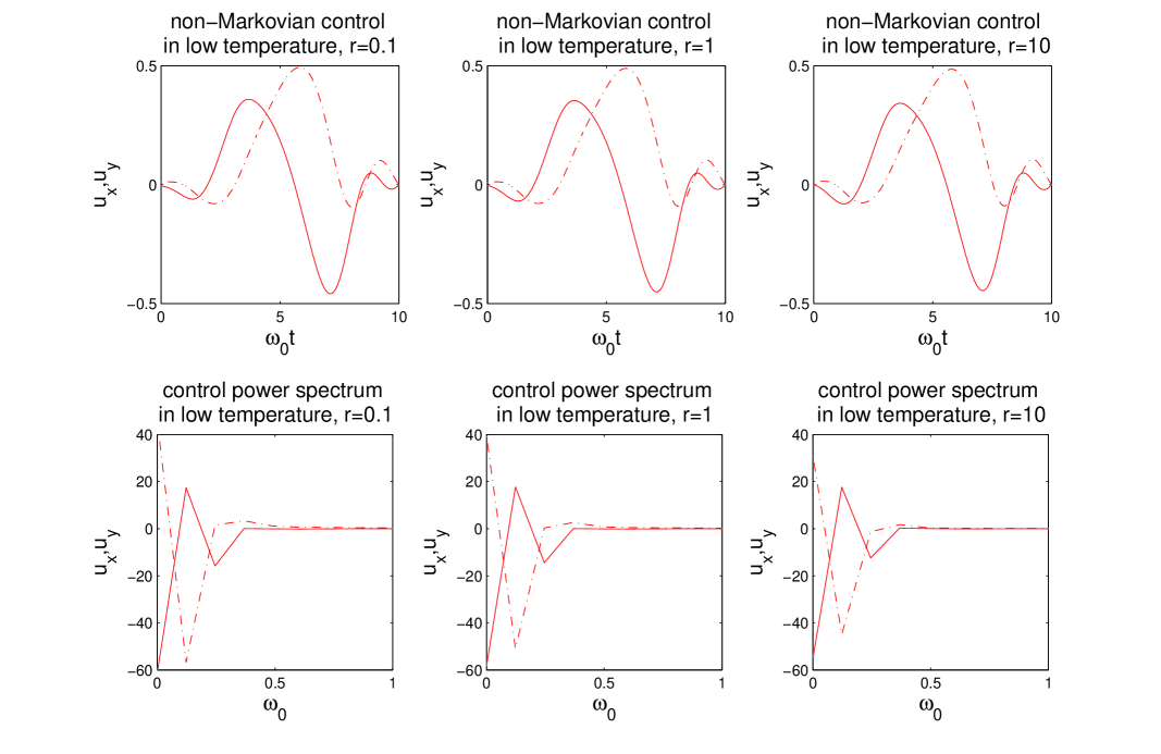
Figure 7: (Color online)non-Markovian optimal controls and their power spectrum in low temperature reservoir for $r=0.1$, $r=1$, and $r=10$ respectively. Non-Markovian optimal control $u_{x}$(red solid line) $u_{y}$(red dash-dotted line).

IV.3 Engineering Reservoirs

During the last two decades, great advances in laser cooling and trapping experimental techniques have made it possible to trap a single ion and cool it down to very low temperature. These cold trapped ions are the favorite candidates for a physical implementation of quantum computers and realization of the quantum cryptography and quantum teleportation. All of these rely on the persistence of quantum coherence. Myatt ; Turchette are the recent experimental procedures for engineering artificial reservoirs. They showed how to couple a properly engineered reservoirs with the trapped atomic ion’s harmonic motion. They measured the decoherence of superpositions of coherent states and two-Fock-state superpositions in the engineering artificial reservoirs. Several type of engineering artificial reservoirs are simulated, e.g., a high-temperature amplitude reservoir, a zero-temperature amplitude reservoir, and a high-temperature phase reservoir.

From above discussions we find that our optimal decoherence control fields do well in the engineering artificial reservoirs.

TABLE I. Controllability

T&r	Low T	Med T	High T
r=0.1	slow decay	slow decay	controllable(non)
r=1	controllable	uncontrollable	uncontrollable
r=10	controllable	uncontrollable	uncontrollable

Table I shows the controllable property of non-Markovian open, dissipative quantum system. When $r\ll 1$ the system free evolution is with little decoherence at low and intermediate temperature and our optimal control plays an important role in controlling the decoherence phenomenon at high temperature. Moreover, when $r\gg 1$ and $r=1$ our optimal control also plays an important role in controlling the decoherence phenomenon at low temperature. They indicate that these engineered reservoirs could be designed that the coupling and state of the environment can be controlled to slow down the decoherence rate and delay decoherence time.

V conclusions

In the present work, we have studied the optimal control of the decoherence for the non-Markovian open quantum system. In the general formalism we proposed the optimal control problem and derived the corresponding Hamilton-Jacobi-Bellman equation. Usually this kind of problem is difficult to be analytically solved. Then we considered this problem in the non-Markovian two-level system. Through transforming its master equation into the Bloch vector representation we obtained the corresponding differential equation with two-sided boundary values.

Finally, we numerically studied the non-Markovian decoherence control for three different conditions, i.e., $\omega_{0}\ll\omega_{c}$, $\omega_{0}\approx\omega_{c}$, $\omega_{0}\gg\omega_{c}$ in the Ohmic environment whose spectral density is with a Lorentz-Drude cuttoff function. Our numerical results indicated that the decoherence dynamics behaves differently for the different environmental condition which leads to significant distinctness in the time dependent behavior of the dissipation function $\gamma(t)$ and $\Delta(t)$. We regarded temperature as a key factor in the decoherence effect and showed that the decoherence can’t be controlled effectively in high temperature for both the Markovian and non-Markovian. Comparing with the Markovian approximation we believed that it is necessary to consider the non-Markovian quantum system. Most of all, we analyzed the short time, moderate time, and long time decoherence control behaviors for $r=0.1$, which implies $\omega_{c}\ll\omega_{0}$. In this case the decoherence can be controlled effectively, which may indicates that the decoherence rate can be slowed down and decoherence time can be delayed through designing some engineered reservoirs proposed by Myatt et. al.

V.1 Comparing the non-Markovian dynamics with the Markovian dynamics

V.1.1 Quantum Markovian Process and Markovian Master Equation

Quantum Markovian process or Markovian approximation is widely used in open quantum system, typically in interaction of radiation with matter (weak coupling); quantum optics and cavity-QED (weak damping); quantum decoherence; quantum Brownian motion (high temperatures); quantum information; quantum error correction; stochastic unravelling (Monte Carlo simulations); laser cooling (Lévy statistics of quantum jumps), and so on. The essence of quantum Markovian process contains three assumptions:

• (i)The initial factorization ansatz (Feynman-Vernon approximation). At time $t=0$ the bath $B$ is in thermal equilibrium and uncorrelated with the system $S$

  $$\begin{split}\rho_{tot}(0)=\rho_{S}(0)\otimes\rho_{B};\end{split}$$ (41)

• (ii)Weak system-bath interaction (Born approximation).

• (iii)Markovian approximation. The relaxation time $\tau_{B}$ of the heat bath is much shorter than the time scale $\tau_{R}$ ($\tau_{B}\ll\tau_{R}$) over which the state of the system varies appreciably.

Then it induced the dynamical map $\Phi_{t}$:

$$\begin{split}\rho_{S}(0)\rightarrow\rho_{S}(t)=\Phi_{t}\rho_{s}(0)=tr_{B}{[U_{t}(\rho_{S}(0)\otimes\rho_{B})U^{{\dagger}}_{t}]}.\end{split}$$ (42)

With some conditions, like completely positive and Hermiticity and trace preservation we get a quantum dynamical semigroup: $\Phi_{t}=exp[\mathcal{L}t],$ which implies the Markovian master equation:

$$\begin{split}\frac{d}{dt}\rho_{s}(t)=\mathcal{L}\rho_{S}(t),\end{split}$$ (43)

where generator of time evolution is in Lindblad form:

$$\begin{split}\mathcal{L}\rho_{S}(t)=-\frac{i}{\hbar}[H_{S},\rho_{S}]+\sum_{i}\gamma_{i}[a_{i}\rho_{S}a_{i}^{{\dagger}}-\frac{1}{2}\{a^{{\dagger}}_{i}a_{i},\rho_{S}\}].\end{split}$$ (44)

V.1.2 Non-Markovian Dynamics and Non-Markovian Master Equation

Non-Markovian dynamics system is not a new research problem, but recently it received considerable consideration H.P.Breuer ; Maniscalco2 ; Breuer1 ; Breuer2 ; Breuer3 . Comparing with the Markovian dynamics it has three properties: (i)Semigroup property violated: slow decay of correlations, strong memory effects; (ii)Initial correlations: classically correlated or entangled initial states; (iii)Strong couplings and low temperatures, with which we can studied the short-time behavior and exact evolution of quantum decoherence. With the help of these three properties we can derive effective equations (Master equations). As far as we known, there are two ways to derive the master equation. One is called the path-integral method by Halliwell et.al Halliwell96 , Hu et. al Hu92 , Ford et. alford01 , and Karrlein et.alkarrlein , the other is the projection operator method by H.P. Breuer H.P.Breuer ; Breuer1 ; Breuer2 ; Breuer3 .

The projection operator method is also called the Nakajima-Zwanzig projection. The basic idea of the technique is to define a map $\mathcal{P}$ as

$$\begin{split}\mathcal{P}{\rho}=tr_{B}\{\rho\}\otimes\rho_{B},\end{split}$$ (45)

where $\rho_{B}$ is a fixed environment state and the map $\mathcal{P}$ is a projection super-operator acting on operators, i.e., $\mathcal{P}^{2}=\mathcal{P}.$ Its complementary projection is

$$\begin{split}\mathcal{Q}=\mathcal{I}-\mathcal{P},\end{split}$$ (46)

where $\mathcal{I}$ is the identity map. Thus the Nakajima-Zwanzig equation can be derived Breuer3 :

$$\begin{split}\frac{d}{dt}\mathcal{P}\rho(t)=\int_{0}^{t}dsK(t,s)\mathcal{P}\rho(s)+\mathcal{I}(t)\mathcal{Q}\rho(0),\end{split}$$ (47)

where $K(t,s)$ is the memory kernel. To second order in the coupling constant the general form of the master equation can be approximated by

$$\begin{split}\frac{d}{dt}\mathcal{P}\rho(t)=\mathcal{K}(t)\mathcal{P}\rho(t)+\mathcal{I}(t)\mathcal{Q}\rho(0).\end{split}$$ (48)

In general, the TCL generator is

$$\begin{split}\mathcal{K}(t)\rho_{S}=-\frac{i}{\hbar}[H_{S}(t),\rho_{S}]+\sum_{i}[C_{i}(t)\rho_{S}D_{i}^{{\dagger}}(t)+D_{i}(t)\rho_{S}C_{i}^{{\dagger}}(t)]-\frac{1}{2}\sum_{i}\{D_{i}^{{\dagger}}(t)C_{i}(t)+C_{i}^{{\dagger}}D_{i}(t),\rho_{S}\},\end{split}$$ (49)

where $C_{i}(t)\neq D_{i}(t)$, which means that it is not in the Lindblad form.

References

- (1) H.P. Breuer, and F. Petruccione, The Theory of Open Quantum Systems, Oxford University Press, Oxford, 2002.
- (2) J. Zhang, C.W. Li, R.B. Wu, T.J. Tarn, and X.S. Liu, J. Phys. A: Math. Gen. 38, 6587(2005).
- (3) S. Lloyd, and J-J. E. Slotine, Phys. Rev. Lett. 80, 4088(1998)
- (4) P. Zanardi, and M. Rasetti, Phys. Rev. Lett. 79, 3306(1997)
- (5) I. L. Chuang, and Y. Yamamoto, Phys. Rev. A. 52, 3489(1995)
- (6) R. Alicki, M. Horodecki, P. Horodecki, and R. Horodecki, Phys. Rev. A, 65, 062101(2002).
- (7) P. Zanardi, Phys. Rev. A 63, 012301(2001).
- (8) J.Von. Neumann, Mathematical Foundations of Quantum Mechanics, Princeton University Press, 1955.
- (9) M.A. Nielsen, and I.L. Chuang, Quantum Computation and Quantum Information, Cambridge University Press, Cambridge, 2000.
- (10) M.B. Mensky, Quantum Menseurements and Decoherence: Models and Phenomenology, Kluwer Academic Publishers, Dordrecht, 2000.
- (11) P.W. Shor, Phys. Rev. A 52, 2493(1995)
- (12) L. Viola, and S. Lloyd, Phys. Rev. A 58, 2733(1998).
- (13) B. Elattari, and S.A. Gurvitz, Phys. Rev. Lett. 84, 2047(2000).
- (14) C. Altafini, J. Math. Phys. 44, 2357 (2003).
- (15) H. Rabitz, R. de ViVie-Riedle, M. Motzkus, and K. Kompa, Science 288, 824(2000).
- (16) R.J. Levis, G.M. Menkir, and H. Rabitz, Science 292, 709(2001).
- (17) H. Rabitz, Science 299, 525(2003).
- (18) V.F. Krotov, Global Methods in Optimal Control Theory, Marcel Dekker INC, New York, (1996).
- (19) H. Jirari, and W. Pötz, Phys. Rev. A 74, 022306(2006).
- (20) D. Sugny, C. Kontz, and H. R. Jauslin, Phys. Rev. A 76, 023419(2007).
- (21) C.W. Gardiner, and P. Zoller, Quantum Noise (2nd Edition), Springer-Verlag, Berlin Heidelberg New York, 2000.
- (22) W.H. Zurek, Rev. Mod. Phys. 75, 715(2003).
- (23) B.M. Garraway, Phys. Rev. A 55, 2290(1997).
- (24) C. J. Myatt, B. E. King, Q. A. Turchette, C. A. Sackett, D. Kielpinski, W. M. Itano, C. Monroe, and D. J. Wineland, Nature(London) 403, 269(2000).
- (25) Q. A. Turchette, C. J. Myatt, B. E. King, C. A. Sackett, D. Kielpinski, W. M. Itano, C. Monroe, and D. J. Wineland, Phys. Rev. A 62, 053807(2000).
- (26) A. Shabani and D. A. Lidar, Phys. Rev. A 71, 020101(2005).
- (27) J.J. Halliwell and T. Yu, Phys. Rev. D 53, 2012 (1996).
- (28) J. Zhang, R.B. Wu, C.W. Li, T.J. Tarn, and J.W. Wu, Phy. Rev. A75, 022324(2007).
- (29) K. Blum, Density Matrix Theory and Applications, Plenum Press, New York, (1981).
- (30) M. Thorwart, L. Hartmann, I. Goychuk, and P. Hänggi, J. Mod. Opt. 47,(2000).
- (31) M. Grifoni, and P. Hänggi, Phys. Rep. 304, (1998).
- (32) J. S. Shao, C. Zerbe, and P. Hänggi, Chem. Phys. 235,(1998).
- (33) I. Goychuk, and P. Hänggi, Chem. Phys. 324, (2006).
- (34) M. Ban, S.Kitajima, and F. Shibata, Phys. Rev. A 76, 022307(2007)
- (35) M. O. Scully, and M. S. Zubairy, Quantum Optics, Cambridge University Press, Cambridge, (1997).
- (36) P. Meystre, Atom Optics, Springer-Verlag, New York, (2001).
- (37) C. Anastopoulos, and B. L. Hu, Phys. Rev. A 62, 033821 (2000).
- (38) S. Shresta, C. Anastopoulos, A. Dragulescu, and B. L. Hu, Phys. Rev. A 71, 022109 (2005).
- (39) B.L. Hu, J.P. Paz, and Y. Zhang, Phys. Rev. D 45, 2843 (1992).
- (40) U. Weiss, Quantum Dissipative System, World Scientific Publishing, Singapore (1993).
- (41) A. J. Leggett, S. Chakravarty, A. T. Dorsey, M. P. A. Fisher, A. Garg, and W. Zwerger, Rev. Mod. Phys. 59, 1(1987).
- (42) J. H. An, W. M. Zhang, Phys. Rev. A 76, 042127 (2007).
- (43) S. Maniscalco, S. Olivares, and M. G. A. Paris, Phys. Rev. A 75, 062119 (2007).
- (44) H.P. Breuer, B.Kappler, and F. Petruccione, Ann. Phys.(N.Y.)291, 36(2001).
- (45) H.P. Breuer, D. Burgarth, and F. Petruccione, Phys. Rev. B70, 045323(2004).
- (46) H.P. Breuer, Phy. Rev. A75, 022103(2007).
- (47) G.W. Ford, and R.F. O’Connel, Phys. Rev. D 64, 105020(2001).
- (48) S. Maniscalco, J.Piilo, F. Petruccione, and A. Messina Phys. Rev. A 70, 032113(2004).
- (49) R. Karrlein and H. Grabert Phys. Rev. E 55, 153(1997).