Gravitational waveforms from unequal-mass binaries with arbitrary spins under leading order spin-orbit coupling

Abstract

The paper generalizes the structure of gravitational waves from orbiting spinning binaries under leading order spin-orbit coupling, as given in the work by Königsdörffer and Gopakumar [PRD 71, 024039 (2005)] for single-spin and equal-mass binaries, to unequal-mass binaries and arbitrary spin configurations. The orbital motion is taken to be quasi-circular and the fractional mass difference is assumed to be small against one. The emitted gravitational waveforms are given in analytic form.

I Introduction

As already stated in many publications before, gravitational waves from inspiralling compact binaries are the most promising sources for ground based planned and already operating gravitational wave (GW) detectors. To guarantee successful search for GWs, one needs to obtain promising search templates incorporating all important physical effects that have an influence on the form of the signal. Ground-based detector networks like LIGO (USA), VIRGO (France/Italy) and GEO 600 (Germany/UK) have the sensitivity to be able to see the last seconds or minutes of the binary’s inspiral, where the corrections, coming from general relativity, to the Newtonian orbital motion get important, depending on their masses. In order to detect GWs from inspiralling compact binaries without spin in quasi-circular orbits, a large library of ready-to-use inspiral templates has been put up DIS . Eccentric inspiral models without spin have also been developed WEX_SCH ; DGI2004 and are well understood. Recently, Yunes and collaborators obtained a formalism for frequency domain GW filters for eccentric binaries Yunes09_ecc_FD . All of them heavily employ the post Newtonian (PN) approximation to general relativity.

It has been shown by several authors, that for a successful detection, effects of spin have to be included and foundations for the detection of spins have been laid down rapid_Kidder_Will ; CutFlan94 ; BCV03 ; BCV05 ; Apost95 . During the inspiral phase, before reaching the last stable orbit, those effects are long-term modulations of the GW signal in a comparison with the time scale of only one orbit. They can lead to substantially different shapes of the signal compared to those ones showing up if the spins are neglected. The foundations for the motion of spins in curved spacetimes are given in PapapetrouI . In harmonic coordinates, the spin dependent EOM were derived up to next-to-leading order in the spin-orbit coupling by Faye et al. BBFI and Blanchet et al. BBFII , where velocities have been used to characterize the orbits. In Arnowitt-Deser-Misner coordinates ADM , higher order Hamiltonians dictating the equations of motion for orbits and spin (from this point on referred to as EOM) have recently been derived by Damour et al. DJS08 and Steinhoff et al. SSH08 ; SHS08 . The spin-independent part of the binary Hamiltonian is known to 3PN order DJS Phys. Lett. B .
The solution to “simple precession” of the leading order spin-orbit interaction, which was the case for single spin or equal mass, was discussed in Apost95 and later in KG05 , where the GW polarizations $h_{\times}$ and $h_{+}$ were derived as a PN accurate analytic solution for eccentric orbits. The latter has heavily inspired this work, which will give an approach to the more general case of unequal masses and arbitrary two-spin configurations.
The paper will be organized as follows. Section II will present the involved Hamiltonians and the associated EOM for the binary in the center-of-mass frame. In section III, the geometry and the coordinates relating the generic reference frame with the orientation of the spins and the angular momentum vector are provided and characterized by rotation matrices. The time derivatives of these rotation matrices will be compared by Poisson brackets in section IV and first order time derivatives of the associated rotation angles will be obtained. A first-order perturbative solution to the EOM for the spins is worked out in section V. The orbital motion will be computed, for quasi-circular orbits (circular orbits in the precessing orbital plane), in section VI. As an application, the resulting GW polarizations, $h_{\times}$ and $h_{+}$ in the quadrupolar restriction, are given in section VII.

II The conservative equations of motion for the spins

In this section the dynamics of spinning compact binaries is investigated where the spin contributions are restricted to the leading order gravitational coupling. The Hamiltonian associated therewith reads

$${\cal H} ={\cal H}_{\rm N}+{\cal H}_{\rm 1PN}+{\cal H}_{\rm 2PN}+{\cal H}_{\rm SO}\,,$$ (1)

with ${\cal H_{\rm N}}$, ${\cal H_{\rm 1PN}}$ and ${\cal H_{\rm 2PN}}$ respectively are the Newtonian, first and second PN order contributions to the conservative point particle dynamics (e.g., Jaran_Schaefer and references therein) and ${\cal H}_{\rm SO}$ is the leading order spin-orbit Hamiltonian Bark_O'ConnI .

In the following computations, use will be made of the following scalings to convert the quantities in calligraphic letters to dimensionless ones on the rhs:

$$\hskip 55.50595pt{\cal H}~{}=~{} {H}\,{\mu c^{2}}\,,$$ (2)

$${\cal R}~{}=~{} \boldsymbol{r}\,\frac{G\,m}{c^{2}}\hrulefill\,,$$ (3)

$${\cal P}~{}=~{} \boldsymbol{p}\,\mu\,c\,,$$ (4)

$${\cal S}_{a}~{}=~{} \boldsymbol{S}_{a}\frac{G\,m_{a}}{c^{2}}\,(m_{a}\,c)\,,$$ (5)

where $m_{a}$ is the mass of the $a^{th}$ object ($a={1,2}$), $m$ is the total mass, $m=m_{1}+m_{2}$, $\mu$ is the reduced mass defined as $m_{1}\,m_{2}/m$ and the symmetric mass ratio is given by $\eta:=m_{1}\,m_{2}/m^{2}$. The variables $\boldsymbol{p}$ and $\boldsymbol{r}$ are the scaled linear canonical momentum and position vectors, respectively, and commute with the spins ${\cal S}_{a}$. Explicitly, the contributions to the scaled version of Eq. (1) read

$${H}(\boldsymbol{r},\boldsymbol{p},\boldsymbol{S}_{1},\boldsymbol{S}_{2}) = {H}_{\rm N}(\boldsymbol{r},\boldsymbol{p})+{H}_{\rm 1PN}(\boldsymbol{r},\boldsymbol{p})+{H}_{\rm 2PN}(\boldsymbol{r},\boldsymbol{p})$$ (6)

$$+~{}{H}_{\rm SO}(\boldsymbol{r},\boldsymbol{p},\boldsymbol{S}_{1},\boldsymbol{S}_{2})\,,$$

with

$${H}_{\rm N}(\boldsymbol{r},\boldsymbol{p}) =\frac{\boldsymbol{p}^{2}}{2}-\frac{1}{r}\,,$$ (7a)

$${H}_{\rm 1PN}(\boldsymbol{r},\boldsymbol{p}) =\frac{1}{c^{2}}\left\{\frac{1}{8}(3\eta-1)\left(\boldsymbol{p}^{2}\right)^{2}-\frac{1}{2}\left[(3+\eta){\boldsymbol{p}}^{2}+\eta(\boldsymbol{n}\cdot\boldsymbol{p})^{2}\right]\frac{1}{r}+\frac{1}{2r^{2}}\right\}\,,$$ (7b)

$${H}_{\rm 2PN}(\boldsymbol{r},\boldsymbol{p}) =\frac{1}{c^{4}}\left\{\frac{1}{16}\left(1-5\eta+5\eta^{2}\right)\left({\boldsymbol{p}}^{2}\right)^{3}+\frac{1}{8}\left[\left(5-20\eta-3\eta^{2}\right)\left({\boldsymbol{p}}^{2}\right)^{2}-2\eta^{2}(\boldsymbol{n}\cdot\boldsymbol{p})^{2}{\boldsymbol{p}}^{2}-3\eta^{2}(\boldsymbol{n}\cdot\boldsymbol{p})^{4}\right]\frac{1}{r}\right.$$

$$\quad\left.+\frac{1}{2}\left[(5+8\eta){\boldsymbol{p}}^{2}+3\eta(\boldsymbol{n}\cdot\boldsymbol{p})^{2}\right]\frac{1}{r^{2}}-\frac{1}{4}(1+3\eta)\frac{1}{r^{3}}\right\}\,,$$ (7c)

$${H}_{\rm SO}(\boldsymbol{r},\boldsymbol{p},\boldsymbol{S}_{1},\boldsymbol{S}_{2}) =\frac{1}{c^{2}r^{3}}(\boldsymbol{r}{\times}\boldsymbol{p})\cdot\boldsymbol{S}_{\text{eff}}\,,$$ (7d)

where $r\equiv|\boldsymbol{r}|$ and $\boldsymbol{S}_{\text{eff}}$ is the so-called effective spin,

$$\boldsymbol{S}_{\text{eff}} \equiv\delta_{1}\boldsymbol{S}_{1}+\delta_{2}\boldsymbol{S}_{2}\hfil\,,$$ (8a)

$$\delta_{1} \equiv\frac{\eta}{2}+\frac{3}{4}\left(1+\sqrt{1-4\eta}\right)\,,$$ (8b)

$$\delta_{2} \equiv\frac{\eta}{2}+\frac{3}{4}\left(1-\sqrt{1-4\eta}\right)\,.$$ (8c)

Considering only the spin-independent part of the Hamiltonian, the orbital angular momentum vector is a conserved quantity. The motion of the reduced mass $\mu$ will, without SO interactions, take place in a plane that is perpendicular to $\boldsymbol{L}$ and that is invariant in time. Adding the spin-orbit term will, in general, lead to a precession of the orbital angular momentum. The EOM for $\boldsymbol{L}$, defined by $\boldsymbol{L}:=\boldsymbol{r}\times\boldsymbol{p}$ and the individual spins $\boldsymbol{S_{1}}$ & $\boldsymbol{S_{2}}$ can be deduced from the equations

$$\frac{d\boldsymbol{L}}{dt} =\{\boldsymbol{L},{H}_{\text{SO}}\}=\frac{1}{c^{2}r^{3}}\boldsymbol{S}_{\text{eff}}\times\boldsymbol{L}\,,$$ (9a)

$$\frac{d\boldsymbol{S}_{1}}{dt} =\{\boldsymbol{S}_{1},{H}_{\text{SO}}\}=\frac{\delta_{1}}{c^{2}r^{3}}\boldsymbol{L}\times\boldsymbol{S}_{1}\,,$$ (9b)

$$\frac{d\boldsymbol{S}_{2}}{dt} =\{\boldsymbol{S}_{2},{H}_{\text{SO}}\}=\frac{\delta_{2}}{c^{2}r^{3}}\boldsymbol{L}\times\boldsymbol{S}_{2}\,.$$ (9c)

Equation (9a) describes the precession of $\boldsymbol{L}$ w.r.t. the total angular momentum vector $\boldsymbol{J}$, defined as $\boldsymbol{J}~{}\equiv~{}\boldsymbol{L}~{}+~{}\boldsymbol{S}_{1}~{}+~{}\boldsymbol{S}_{2}$. The key idea in the next sections is to compute time dependent rotation matrices for $\boldsymbol{L}$, $\boldsymbol{S}_{1}$ and $\boldsymbol{S}_{2}$ for a number of rotation axes and angles that are to be introduced in the next section. Let us state that the magnitudes $L$, $S_{1}$ and $S_{2}$ of the vectors $\boldsymbol{L}$, $\boldsymbol{S}_{1}$ and $\boldsymbol{S}_{2}$ are conserved,

$$\frac{d{L}^{2}}{dt}= ~{}\frac{d}{dt}(\boldsymbol{L}\cdot\boldsymbol{L})=\frac{2}{c^{2}r^{3}}\boldsymbol{L}\cdot(\boldsymbol{S}_{\text{eff}}\times\boldsymbol{L})=0\,,\,$$ (10a)

$$\frac{dS_{1}^{2}}{dt}= ~{}\frac{d}{dt}(\boldsymbol{S}_{1}\cdot\boldsymbol{S}_{1})=\frac{2\delta_{1}}{c^{2}r^{3}}\boldsymbol{S}_{1}\cdot(\boldsymbol{L}\times\boldsymbol{S}_{1})=0\,,~{}\,$$ (10b)

$$\frac{dS_{2}^{2}}{dt}= ~{}\frac{d}{dt}(\boldsymbol{S}_{2}\cdot\boldsymbol{S}_{2})=\frac{2\delta_{2}}{c^{2}r^{3}}\boldsymbol{S}_{2}\cdot(\boldsymbol{L}\times\boldsymbol{S}_{2})=0\,.\,$$ (10c)

Equations (9) show that $\dot{\boldsymbol{L}}=-(\dot{\boldsymbol{S}}_{1}+\dot{\boldsymbol{S}}_{2})$ and, thus, the total angular momentum vector $\boldsymbol{J}$ satisfies

$$\frac{d\boldsymbol{J}}{dt}=0~{}\text{, giving}~{}\frac{d|\boldsymbol{J}|}{dt}=0\,.$$ (11)

The magnitudes of $\boldsymbol{S}$ and $\boldsymbol{S_{\text{eff}}}$ behave as follows,

$$\frac{dS^{2}}{dt} =-\frac{3\sqrt{1-4\eta}}{c^{2}r^{3}}\boldsymbol{L}\cdot(\boldsymbol{S}_{1}\times\boldsymbol{S}_{2})\,,$$ (12a)

$$\frac{dS^{2}_{\text{eff}}}{dt} =-\frac{3\sqrt{1-4\eta}\,(12+\eta)\eta}{4c^{2}r^{3}}\boldsymbol{L}\cdot(\boldsymbol{S}_{1}\times\boldsymbol{S}_{2})\,.$$ (12b)

Notice the conservation of $S^{2}_{\text{eff}}$ in both the test-mass ($\eta=0$) and equal-mass ($\eta=1/4$) cases. Using above equations, we will be able to compute the evolution equations for the rotation angles. The associated geometry is introduced next.

III Geometry of the binary

As done in KG05 , it is very useful to use a fixed orthonormal frame ($\boldsymbol{e_{X}},\boldsymbol{e_{Y}},\boldsymbol{e_{Z}}$) and to set $\boldsymbol{e_{Z}}$ along the fixed vector $\boldsymbol{J}$. The invariable plane perpendicular to $\boldsymbol{J}$ will then be spanned by the vectors ($\boldsymbol{e_{X}},\boldsymbol{e_{Y}}$). The motion of the reduced mass will take place in the orbital plane perpendicular to the unit vector $\boldsymbol{k}:=\boldsymbol{L}/L$. For a clear understanding of the following, please take a look at Fig. 1. First, the vector $\boldsymbol{k}$ is inclined to $\boldsymbol{e_{Z}}$ by the (time-dependent) angle $\Theta$, which was also the constant precession cone of $\boldsymbol{L}$ around $\boldsymbol{J}$ for the single-spin and equal-mass case of KG05 . As before, the orbital plane, itself spanned by the vectors $(\boldsymbol{i},\boldsymbol{j})$, where $\boldsymbol{j}=\boldsymbol{k}\times\boldsymbol{i}$, intersects the invariable plane at the line of nodes $\boldsymbol{i}$, with the longitude $\Upsilon$ measured in the invariable plane from $\boldsymbol{e_{X}}$.

The geometry of the binary will be completed by the spin related coordinate system $(\boldsymbol{i_{s}},\boldsymbol{j_{s}},\boldsymbol{k_{s}})$. This frame is constructed from the system $(\boldsymbol{i},\boldsymbol{j},\boldsymbol{k})$ to be rotated around the axis $\boldsymbol{i}$ to point from the top of $\boldsymbol{L}$ to the top of $\boldsymbol{J}$ with the new direction $\boldsymbol{k_{s}}$. In other words, this spin coordinate system is chosen in such a way that the total spin, $\boldsymbol{S}_{1}+\boldsymbol{S}_{2}$, has only a $\boldsymbol{k_{s}}$ component and $\boldsymbol{i}_{s}\equiv\boldsymbol{i}$ holds. If $\Theta$ is known, the spins are left with an additional freedom to rotate around $\boldsymbol{k_{s}}$ by an angle $\phi_{s}$ (the index “s” is a hint for positions in the spin system). This angle is measured from $\boldsymbol{i_{s}}$ to the projection of $\boldsymbol{S}_{1}$ to the $(\boldsymbol{i_{s}},\boldsymbol{j_{s}})$ plane, similar to $\Upsilon$’s function in the reference frame.

There exist simple geometrical relations that will reduce the freedom to choose rotation angles arbitrarily, as will be shown in the next subsection.

III.1 Geometrical issues

As mentioned already, in this geometry the spins and angular momenta – being fixed in their magnitudes – only have three degrees of freedom: the angles $\Theta$, $\Upsilon$ and $\phi_{s}$. Once $\Theta$ is determined, also $\alpha_{\text{ks}}$ (the angle between $\boldsymbol{L}$ and $\boldsymbol{S}$) is fixed and so is magnitude $S$ of $\boldsymbol{S}=\boldsymbol{S}_{1}+\boldsymbol{S}_{2}$ by triangular relations. Calling $\alpha_{12}$ the angle between the spins $\boldsymbol{S}_{1}$ and $\boldsymbol{S}_{2}$, the following equations list the rotation angles and magnitudes as functions of $\Theta$, where also use is made of the sin relations,

$$S(\Theta)=~{} \sqrt{J^{2}-2JL\cos\Theta+L^{2}}\,,$$ (13a)

$$\alpha_{12}(\Theta)=~{} \cos^{-1}\left(\frac{S(\Theta)^{2}-S_{1}^{2}-S_{2}^{2}}{-2S_{1}S_{2}}\right)\,,$$ (13b)

$$\alpha_{\text{ks}}(\Theta)=~{} \pi-\sin^{-1}\left(\frac{J\sin(\Theta)}{\text{S}(\Theta)}\right)\,,$$ (13c)

$$\tilde{s}(\Theta)=~{} \sin^{-1}\left(\frac{S_{2}\sin\alpha_{12}(\Theta)}{\text{S}(\Theta)}\right)\,.$$ (13d)

These relations will be used extensively to simplify the angles evolution equations. How they are incorporated and applied will be shown next.

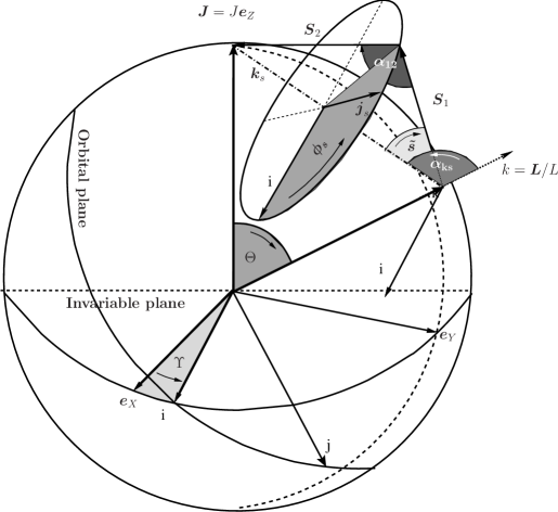
Figure 1: Binary geometry completed by a rotating spin coordinate system. The usual reference frame is ($\boldsymbol{e_{X}},\boldsymbol{e_{Y}},\boldsymbol{e_{Z}}$) having chosen $\boldsymbol{e_{Z}}$ to be aligned with $\boldsymbol{J}$. The vectors $\boldsymbol{L},\boldsymbol{S}_{1},\boldsymbol{S}_{2}$ describe the orbital angular momentum and the individual spins, respectively. The angle $\Theta$ denotes the inclination angle of $\boldsymbol{L}$ w.r.t. $\boldsymbol{J}$, which is – of course – to be taken as a time dependent quantity. The orbital plane, being perpendicular to $\boldsymbol{L}$ by construction, is spanned by the orthonormal vectors $\boldsymbol{j}$ and $\boldsymbol{i}$, where the latter one intersects the invariable plane at the angle $\Upsilon$ measured from $\boldsymbol{e_{X}}$. The spin-coordinate system is constructed out of the orbital dreibein ($\boldsymbol{i},\boldsymbol{j},\boldsymbol{k}$) by a rotation of $\alpha_{\text{ks}}$ around $\boldsymbol{i}$, such that the vector pointing from $\boldsymbol{L}$ to $\boldsymbol{J}$ is the total spin $\boldsymbol{S}_{1}+\boldsymbol{S}_{2}$. The angle $\alpha_{12}$ is measured between $\boldsymbol{S}_{1}$ and $\boldsymbol{S}_{2}$. The spin $\boldsymbol{S}_{1}$, projected into the ($\boldsymbol{j}_{s},\boldsymbol{i}_{s}\equiv\boldsymbol{i}$) plane is rotated by an angle $\phi_{s}$ from $\boldsymbol{i}$, and $\boldsymbol{S}_{1}$ itself is moving on the circle (with variable radius) embedded in the figure.

III.2 Coordinate bases and associated transformation matrixes

This section introduces the coordinate transformations from the reference system to the orbital triad and the spin system. To construct the EOM for the 3 physical angles $\Theta,\Upsilon$ and $\phi_{s}$, the idea is to compare the evolution of these rotation angles - as arguments for rotation matrices - with the Poisson brackets, Eqs. (9a) - (9c). Let us begin with the explicit computation of the transformed coordinate bases.

1. The orbital triad ($\boldsymbol{i},\boldsymbol{j},\boldsymbol{k}$) can be, not surprisingly, constructed by only 2 rotations from the reference system. In terms of rotation matrices, we have

   $$\begin{pmatrix}\boldsymbol{i}\\ \boldsymbol{j}\\ \boldsymbol{k}\end{pmatrix}= \begin{pmatrix}1&0&0\\ 0&\cos\Theta&\sin\Theta\\ 0&-\sin\Theta&\cos\Theta\end{pmatrix}\begin{pmatrix}\cos\Upsilon&\sin\Upsilon&0\\ -\sin\Upsilon&\cos\Upsilon&0\\ 0&0&1\end{pmatrix}$$ (14)

   $$\times\begin{pmatrix}\boldsymbol{e}_{X}\\ \boldsymbol{e}_{Y}\\ \boldsymbol{e}_{Z}\end{pmatrix}\,.$$

2. The spin system is constructed, simply by another rotation of $\alpha_{\text{ks}}$ around the vector $\boldsymbol{i}$, from the orbital triad,

   $$\begin{pmatrix}\boldsymbol{i_{s}}\\ \boldsymbol{j_{s}}\\ \boldsymbol{k_{s}}\end{pmatrix} =\begin{pmatrix}1&0&0\\ 0&\cos\alpha_{\text{ks}}&-\sin\alpha_{\text{ks}}\\ 0&\sin\alpha_{\text{ks}}&~{}\cos\alpha_{\text{ks}}\end{pmatrix}\begin{pmatrix}\boldsymbol{i}\\ \boldsymbol{j}\\ \boldsymbol{k}\end{pmatrix}\,,$$ (15)

   such that $\boldsymbol{i_{s}}\equiv\boldsymbol{i}$ holds. Important note: the angle $\alpha_{\text{ks}}$ has negative sign relative to $\Theta$. That’s because $\boldsymbol{k_{s}}$ has to be moved “backwards” to point to $\boldsymbol{J}$!

Having transformed the unit vectors with these matrices, the coordinates transform by their transposed inverses, which are – in case of rotations – the matrices themselves.

Now, we have everything under control to construct the set of all the physical vectors. I will list all of them below. First, let me define some shorthands for rotation matrices:

$$\left[\Theta\right] \equiv ~{}\begin{pmatrix}1&0&0\\ 0&\cos\Theta&\sin\Theta\\ 0&-\sin\Theta&\cos\Theta\end{pmatrix}\,,$$ (16)

$$\left[\Upsilon\right] \equiv ~{}\begin{pmatrix}\cos\Upsilon&\sin\Upsilon&0\\ -\sin\Upsilon&\cos\Upsilon&0\\ 0&0&1\end{pmatrix}\,,$$ (17)

$$\left[\alpha_{\text{ks}}\right] \equiv ~{}\begin{pmatrix}1&0&0\\ 0&\cos\alpha_{\text{ks}}&-\sin\alpha_{\text{ks}}\\ 0&\sin\alpha_{\text{ks}}&~{}\cos\alpha_{\text{ks}}\end{pmatrix}\,.$$ (18)

The orbital angular momentum $\boldsymbol{L}$ in the reference system (indices labeled inv) arises from two rotations from the orbital triad (ot) where it has only one component:

$$\boldsymbol{L}=\left\{\left[\Theta(t)\right]\,\left[\Upsilon(t)\right]\right\}^{-1}(0,0,L)\,,$$ (19)

or, in components,

$$(\boldsymbol{L})_{i}^{\text{\rm{inv}}}=\biggl{\{}~{}\left[\Theta(t)\right]\left[\Upsilon(t)\right]~{}\biggr{\}}^{-1}_{ij}(\boldsymbol{L})_{j}^{\text{\rm{ot}}}\,.$$ (20)

The spins, in the spin system (s), where the $\boldsymbol{k_{s}}$ is aligned with $\boldsymbol{S}=\boldsymbol{S}_{1}+\boldsymbol{S}_{2}$, have the following form,

$$\boldsymbol{S}_{1}=~{} S_{1}(\cos\phi_{s}\sin\tilde{s}~{}\boldsymbol{i_{s}}+\sin\phi_{s}\sin\tilde{s}\,\boldsymbol{j_{s}}+\cos\tilde{s}\,\boldsymbol{k_{s}})\,,$$ (21a)

$$\boldsymbol{S}_{2}=~{} S\,\boldsymbol{k_{s}}-\boldsymbol{S}_{1}\,,$$ (21b)

$$\boldsymbol{S}=~{} S\,\boldsymbol{k_{s}}\,.$$ (21c)

IV The time derivatives of $\Upsilon$, $\Theta$ and $\phi_{s}$

To obtain an EOM for the angle $\Theta$, one possibility is to use the time derivative of $|S|^{2}=(\boldsymbol{S}\cdot\boldsymbol{S})$, Eq. (12a), to apply this, for example, in the spin system and to compare the result with the time derivative of Eq. (13a) with $\Theta=\Theta(t)$. The result is

$$\dot{\Theta}=-\frac{C_{\text{S}}S_{1}S}{2J}\,\sin\alpha_{\text{ks}}\cos\phi_{s}\sin\tilde{s}\csc\Theta$$ (22)

with

$${C_{\text{S}}=-\frac{3\sqrt{1-4\eta}}{c^{2}r^{3}}}\,.$$ (23)

The same result will be obtained by computing the time derivative of the orbital angular momentum $\boldsymbol{L}$ in the invariable system. Therefore, take Eq. (19), compute its time derivative and finally compare the result with (9a). Because the angular velocities appear in relatively simple relations, it is easy to extract them from the $\boldsymbol{e_{X}}$ and $\boldsymbol{e_{Y}}$ entry. The results are

$$\dot{\Upsilon} = -~{}{C_{L}}\csc\Theta\,\left[S_{1}(\delta_{2}-\delta_{1})\cos\alpha_{\text{ks}}\sin\phi_{s}\sin\tilde{s}+\sin\alpha_{\text{ks}}(S_{1}(\delta_{1}-\delta_{2})\cos\tilde{s}+{S}\delta_{2})\right]\,,$$ (24)

$$\dot{\Theta} = C_{L}\,S_{1}(\delta_{1}-\delta_{2})\cos\phi_{s}\,\sin\tilde{s}\,,$$ (25)

with $C_{L}:=(c^{2}\,r^{3})^{-1}$ . The functional dependencies of $\alpha_{\text{ks}}$, $\tilde{s}$ and $S$ on $\Theta$ are implicated. Inserting the geometrical relations, Eqs. (13), it turns out that Eqs. (22) and (25) are equivalent. Also, the allegedly worrying asymmetric appearance of the quantity $S_{1}$ can be studiously avoided by replacing $\tilde{s}$ by its function of $\Theta$.

Also note that, if the relations $\eta=1/4$ or $S_{i}=0~{}(i=1\text{ or }2)$ are inserted in Eq. (24), one recovers Eq. (4.32) of KG05 .
Now, let us turn to the last quantity to be determined, the angle $\phi_{s}$. The geometry offers various possibilities to calculate the time derivative of this angle. The easy way is to compute $\boldsymbol{S}_{1}$ in the invariable system. In components, we have

$$(\boldsymbol{S}_{1})_{i}^{\text{\rm{inv}}}=\biggl{\{}\left[\alpha_{\text{ks}}(t)\right]\left[\Theta(t)\right]\left[\Upsilon(t)\right]\biggr{\}}^{-1}_{ij}(\boldsymbol{S}_{1})_{j}^{\text{s}}\,.$$ (26)

The time derivative of (26) might be compared with Eq. (9b). The result will be given in terms of the angles already determined: since we already know $\dot{\Theta}$ and $\dot{\Upsilon}$ on the one hand and $\alpha_{\text{ks}}$ as a function of $\Theta$ on the other, we have the expression under full control.

The other way is to take the Leibniz product rule for $\boldsymbol{S}$, namely $\partial_{t}{\boldsymbol{S}}=\partial_{t}{S^{i}}\,\boldsymbol{e}_{i}+S^{i}\,\partial_{t}{\boldsymbol{e}_{i}}$ with $\boldsymbol{e}_{i}=(\boldsymbol{i_{s}},\boldsymbol{j_{s}},\boldsymbol{k_{s}})$. We we already know that $\boldsymbol{i_{s}}\equiv\boldsymbol{i}$, $\boldsymbol{k_{s}}||\boldsymbol{S}$ and $\boldsymbol{j_{s}}\equiv\boldsymbol{i_{s}}\times\boldsymbol{k_{s}}$, whose time derivatives are already known. Both considerations result in

$$\dot{\phi}_{s}~{}= ~{}{C_{\Theta}}\,(\dot{\Theta}~{}-\dot{\alpha}_{\text{ks}})~{}+{C_{\tilde{s}}}\,\dot{\tilde{s}}~{}+\Omega_{0}\,,$$ (27a)

$${C_{\Theta}}~{}= ~{}\tan\phi_{s}\,\cot({\alpha_{\text{ks}}}-\Theta)+\sec\phi\cot\tilde{s}\,,$$ (27b)

$${C_{\tilde{s}}}~{}= ~{}-\sec\phi_{s}\,\cot({\alpha_{\text{ks}}}-\Theta)-\tan\phi\cot\tilde{s}\,,$$ (27c)

$$\Omega_{0}~{}= ~{}-{C_{1}}\,L\,\sin\Theta\,\csc({\alpha_{\text{ks}}}-\Theta)\,.$$ (27d)

For the case of equal masses ($\delta_{1}=\delta_{2}=\delta=7/8$), one obtains for $\dot{\phi}_{s}$, $\dot{\Upsilon}$ and $\dot{\Theta}$ a very simple system of EOM,

$$\dot{\Theta}= ~{}0\,,$$ (28a)

$$\dot{\Upsilon}= ~{}\frac{7J}{8c^{2}r^{3}}\,,$$ (28b)

$$\dot{\phi}_{s}= ~{}-\frac{L\delta\sin\Theta}{c^{2}r^{3}}\,{\csc\left\{\sin^{-1}\left(\frac{J\sin\Theta}{S(\Theta)}\right)+\Theta\right\}}\,,$$ (28c)

which can be integrated immediately, giving

$$\Theta(t)= ~{}\Theta_{0}\,,$$ (29a)

$$\Upsilon(t)= ~{}\Omega_{\Upsilon}\,t+\Upsilon_{0}\,,$$ (29b)

$$\phi_{s}(t)= ~{}\Omega_{\phi}\,t+{\phi_{s}}_{0}\,,$$ (29c)

with the angular velocities

$$\Omega_{\Upsilon}\equiv \frac{7J}{8c^{2}r^{3}}\,,\hrulefill$$ (30a)

$$\Omega_{\phi}\equiv -\frac{L\delta\sin\Theta_{0}}{c^{2}r^{3}}\,{\csc\left\{\sin^{-1}\left[\frac{J\sin\Theta_{0}}{S(\Theta_{0})}\right]+\Theta_{0}\right\}}\,.$$ (30b)

Summarizing the EOM for the coordinate transformation angles, Eqs. (24), (25) and (27), this system of EOM can be written in a compact manner. Calling the vector of constants, ${\boldsymbol{C}}=\left\{E,S_{1},S_{2},L,\boldsymbol{k}\cdot\boldsymbol{S}_{\text{eff}}\right\}$ – where $E$ and $L$ are related in the case of quasi-circular orbits – and the vector of dynamic variables, associated with spins and angular momentum, ${\boldsymbol{X}}=\left\{\Theta,\Upsilon,\phi_{s}\right\}$, we may write

$$\frac{d}{dt}\,{\boldsymbol{X}}=\boldsymbol{Y}_{\boldsymbol{C}}(\boldsymbol{X})\,.$$ (31)

A perturbative solution will be given in the next section.

V First order perturbative solution to the EOM for the non-equal mass case

The EOM for ($\Theta,\Upsilon,\phi_{s}$) can also be solved by a simple reduction scheme. We assume that the deviation from the equal-mass case is small compared to unity,

$$\frac{\delta_{1}-\delta_{2}}{\delta_{1}+\delta_{2}}\ll 1\,.$$ (32)

Then, having the equal-mass case under full analytic control, we can construct a perturbative solution to the non-equal mass case. The proceeding is as follows: Imagine a system of EOM for a number $N$ of dependent variables $\boldsymbol{X}$:

$$\dot{\boldsymbol{X}}=\boldsymbol{Y}(\boldsymbol{X})\,.$$ (33)

The time domain solution to this system is denoted by the superscript “$0$”, viz

$$\boldsymbol{X}(t)=\boldsymbol{X}^{(0)}(t)\,.$$ (34)

Let us assume that the EOM, Eq. (33), are perturbed by some terms of the order $\epsilon$ ($\epsilon$ is a dimensionless ordering parameter),

$$\dot{\boldsymbol{X}}=\boldsymbol{Y}(\boldsymbol{X})+\epsilon\,\boldsymbol{P}(\boldsymbol{X})\,.$$ (35)

The solution at the first order in $\epsilon$ can be obtained by adding a small perturbed quantity to be determined to the solution of the homogeneous equation,

$$X_{i}^{(1)}(t)=X_{i}^{(0)}(t)+\epsilon\,S_{i}(t)\,.$$ (36)

Inserting this into Eq. (35), one obtains

$$\dot{X}_{i}^{(1)} = \dot{X}_{i}^{(0)}+\epsilon\,\dot{S}_{i}$$ (37)

$$= Y_{i}(X_{j}^{(0)}+\epsilon\,S_{j})+\epsilon\,P_{i}(X_{j}^{(0)}+\epsilon\,S_{j})$$

$$= Y_{i}(X_{j}^{(0)})+\epsilon\,\sum_{j=1}^{N}\frac{\partial Y_{i}}{\partial X_{j}}\,S_{j}$$

$$+\epsilon\,P_{i}(X_{j}^{(0)})+{\cal{O}}(\epsilon^{2})$$

Comparing the coefficients of the two orders of $\epsilon$ gives

$$0: \dot{X}_{i}^{(0)}= Y_{i}(X_{j}^{(0)})\,,$$ (38)

$$1: \dot{S}_{i}= \sum_{j=1}^{N}\frac{\partial Y_{i}}{\partial X_{j}}\,S_{j}+P_{i}(X_{j}^{(0)})\,.$$ (39)

The first equation is solved via definition, and what remains is the second, having inserted the unperturbed solution in the perturbing function $P$. For our purposes, $N=3$ with $\boldsymbol{X}=\{\Upsilon,\Theta,\phi_{s}\}$ is a small number of EOMs, but complicated functional dependencies are included. The matrix appearing in Eq. (39) does not mean a problem to us, because fortunately, the only dependency of the sources is on $\Theta$.

For our computation, we need to divide the EOM into a non-perturbative and a perturbative part. In the following, we use the definitions

$$\chi_{1} = \frac{\delta_{1}+\delta_{2}}{2}\,,$$ (40)

$$\chi_{2} = \frac{\delta_{1}-\delta_{2}}{2}\,.$$ (41)

Rewriting the EOM for the angles in terms of $\chi_{1}$ and $\chi_{2}$, labeling all $\chi_{2}$ contributions with the order parameter $\epsilon$ as well as inserting the non-perturbative solution, Eqs. (29) to these terms, one obtains

$$\dot{\Theta}^{(1)}=\epsilon\dot{S}_{\Theta}= ~{}\epsilon\,C_{L}S_{1}2\,\chi_{2}\cos(t\,\Omega_{\phi}+\phi_{0})\sin\tilde{s}(\Theta_{0})\,,$$ (42a)

$$\dot{\Upsilon}^{(0)}+\epsilon\dot{S}_{\Upsilon}= ~{}\underbrace{C_{L}S(\Theta)\chi_{1}\sin\alpha_{\text{ks}}(\Theta)\csc\Theta}_{\equiv C_{L}J\chi_{1}=\text{const.}}+\epsilon\,\bigl{[}C_{L}\chi_{2}\csc\Theta_{0}\ \bigl{(}2S_{1}\cos\alpha_{\text{ks}}\left(\Theta_{0}\right)\sin{\tilde{s}}\left(\Theta_{0}\right)\sin\left(t\Omega_{\phi}+\phi_{0}\right)$$

$$~{}-\sin\alpha_{\text{ks}}\left(\Theta_{0}\right)\left(S(\Theta_{0})-2S_{1}\cos\tilde{s}(\Theta_{0})\right)\bigr{)}\bigr{]}\,,$$ (42b)

$$\dot{\phi}_{s}^{(0)}+\epsilon\dot{S}_{\phi}= ~{}-C_{1}L\sin\Theta\csc\alpha_{\text{ks}}(\Theta)+\epsilon\,\biggl{[}{C_{\tilde{s}}}(\Theta,\phi_{s})\,\,\frac{\partial\tilde{s}}{\partial\Theta}+{C_{\Theta}}(\Theta,\phi_{s})\,\left(1-\frac{\partial\alpha_{\text{ks}}}{\partial\Theta}\right)\biggr{]}~{}\vline~{}_{{}^{\Theta=\Theta_{0}}_{\phi_{s}=t\,\Omega_{\phi}+{\phi_{s}}_{0}}}\,\dot{\Theta}\,,$$ (42c)

$$= ~{}-(\chi_{1}+\epsilon\,\chi_{2})\frac{L}{c^{2}r^{3}}\sin\Theta\csc\alpha_{\text{ks}}(\Theta)+\epsilon\,\biggl{[}{C_{\tilde{s}}}(\Theta,\phi_{s})\,\frac{\partial\tilde{s}}{\partial\Theta}+{C_{\Theta}}(\Theta,\phi_{s})\,\left(1-\frac{\partial\alpha_{\text{ks}}}{\partial\Theta}\right)\biggr{]}~{}\vline~{}_{{}^{\Theta=\Theta_{0}}_{\phi_{s}=t\,\Omega_{\phi}+{\phi_{s}}_{0}}}\,\dot{\Theta}\,.$$ (42d)

The parameter $\epsilon$ simply counts the order of the perturbative contribution and is later set to one. The first term for $\Upsilon$ is constant and thus does not have to be expanded in powers of $\epsilon$, but the associated first term for $\phi_{s}$ does, such that the perturbative solution for $\Theta$ has to be included. Taylor expanding this term, removing all contributions to the unperturbed problem, what remains is a system of EOM for $S_{\Theta},S_{\Upsilon},S_{\phi}$ that can be simply integrated, because as soon as $S_{\Theta}(t)$ is known, all the other contributions are straightforwardly evaluated. Requiring that the perturbing solutions vanish at $t=0$, the solutions are simply given by

$$S_{\Theta}(t) =\int_{0}^{t}\dot{S}_{\Theta}dt\,,$$ (43a)

$$S_{\Upsilon}(t) =\int_{0}^{t}\dot{S}_{\Upsilon}dt\,,$$ (43b)

$$S_{\phi}(t) =\int_{0}^{t}\dot{S}_{\phi}dt\,,$$ (43c)

and explicitly read

$$S_{\Theta}(t)= ~{}-\frac{C_{L}S_{1}S_{2}2\chi_{2}}{S_{(0)}\Omega_{\phi}}\,{\sin\alpha_{12}}_{(0)}\left(\sin{\phi_{s}}_{0}-\sin\left(t\Omega_{\phi}+{\phi_{s}}_{0}\right)\right)\,,$$ (44a)

$$S_{\Upsilon}(t)= ~{}\frac{{C_{L}}{\chi_{2}}\csc\Theta_{0}}{\Omega_{\phi}}\biggl{[}2S_{1}\cos{\alpha_{\text{ks}}}_{(0)}\sin\tilde{s}_{(0)}\left(\cos{\phi_{s}}_{0}-\cos\left(t\Omega_{\phi}+{\phi_{s}}_{0}\right)\right)$$

$$~{}-t\Omega_{\phi}\sin{\alpha_{\text{ks}}}_{(0)}\left(S_{(0)}-2S_{1}\cos\tilde{s}_{(0)}\right)\biggr{]}\,,$$ (44b)

$$S_{\phi}(t)= ~{}C_{\text{stat}}\,t+C_{0}(t)+C_{\tilde{s}}(t)+C_{\Theta}(t)+C_{\alpha}(t)\,,$$ (44c)

with the shorthands

$$C_{\text{stat}}= ~{}\frac{\chi_{2}\Omega_{\phi}}{\chi_{1}}\,,$$ (45a)

$$C_{0}(t)= ~{}\frac{{C_{L}}JS_{1}S_{2}\chi_{2}\sin\Theta_{0}\sin{\alpha_{12}}_{(0)}\left(t\Omega_{\phi}\sin{\phi_{s}}_{0}+\cos\left(t\Omega_{\phi}+{\phi_{s}}_{0}\right)-\cos\phi_{0}\right)\left(-2c^{2}Jr^{3}\Omega^{*}-2\chi_{1}S_{(0)}^{2}\right)}{\chi_{1}S_{(0)}^{3}\Omega_{\phi}\sqrt{S_{(0)}^{2}-J^{2}\sin^{2}\Theta_{0}}}\,,$$ (45b)

$$C_{\tilde{s}}(t)= ~{}\frac{-2{C_{L}}J\chi_{2}\left(S_{(0)}^{2}\cot{\alpha_{12}}_{(0)}-S_{1}S_{2}\sin{\alpha_{12}}_{(0)}\right)}{\chi_{1}S_{(0)}^{2}\Omega_{\phi}\sqrt{S_{(0)}^{2}-S_{2}^{2}\sin^{2}{\alpha_{12}}_{(0)}}}\times$$

$$~{}{\left(c^{2}r^{3}t\Omega_{\phi}\sin\tilde{s}_{(0)}\Omega^{*}+L\chi_{1}\sin\Theta_{0}\cos\tilde{s}_{(0)}\left(\cos{\phi_{s}}_{0}-\cos\left(t\Omega_{\phi}+{\phi_{s}}_{0}\right)\right)\right)}\,,$$ (45c)

$$C_{\Theta}(t)= ~{}\frac{2S_{1}t\chi_{2}\cos\tilde{s}_{(0)}}{c^{2}r^{3}}+\frac{2S_{1}\chi_{2}\Omega^{*}\csc\Theta_{0}\sin\tilde{s}_{(0)}\left(\cos{\phi_{s}}_{0}-\cos\left(t\Omega_{\phi}+{\phi_{s}}_{0}\right)\right)}{L\chi_{1}\Omega_{\phi}}\,,$$

$$C_{\alpha}(t)= ~{}C_{\Theta}(t)\,\frac{J\left(S_{(0)}^{2}\cos\Theta_{0}-JL\sin^{2}\Theta_{0}\right)}{S_{(0)}^{2}\sqrt{S_{(0)}^{2}-J^{2}\sin^{2}\Theta_{0}}}\,,$$ (45d)

the initial values of the functions (13a) - (13d)

$$S_{(0)} \equiv S(\Theta_{0})\,,$$ (46a)

$${\alpha_{\text{ks}}}_{(0)} \equiv\alpha_{\text{ks}}(\Theta_{0})\,,$$ (46b)

$${\alpha_{\text{12}}}_{(0)} \equiv\alpha_{\text{12}}(\Theta_{0})\,,$$ (46c)

$${\tilde{s}}_{(0)} \equiv\tilde{s}(\Theta_{0})\,,$$ (46d)

and the definition

$$\Omega^{*} \equiv\Omega_{\phi}\,\sqrt{1-\frac{L^{2}\chi_{1}^{2}\sin^{2}\Theta_{0}}{c^{4}r^{6}\Omega_{\phi}^{2}}}\,.$$ (46f)

VI The orbital motion

The motion of the spins is only half of the physical content of the spin-orbit dynamics. Once we fully have the motion of all the spin-related angles under control, we might turn to the orbital dynamics, i.e. the motion of the reduced mass in the orbital plane. It will turn out that employing coordinate transformations will be very helpful here, too.

The aim is to solve the orbital EOM to the full Hamiltonian,

$${H}=H_{\text{N}}+H_{\text{1PN}}+H_{\text{2PN}}+H_{\text{SO}}\,.$$ (47)

At this point, we can do a useful simplification. As long as we incorporate only leading order spin dynamics, only Newtonian point particle and spin dependent contributions will mix at the end, higher order PN terms coupling with the spins will be neglected consequently. For the computation of the spin dependent part of the orbital phase, therefore, we only have to take ${H}_{\rm N,SO}=H_{\rm N}+H_{\rm SO}$ and add the 1PN and 2PN (spinless) terms for the point particle afterwards.

$$H = {H}_{\rm N,SO}+H_{\rm 1PN}+H_{\rm 2PN}\,,$$ (48)

$$\dot{\varphi} = \dot{\varphi}_{\rm N,SO}+\dot{\varphi}_{\rm 1PN}+\dot{\varphi}_{\rm 2PN}\,.$$ (49)

The Newtonian and spin orbit part of eq. (47) reads

$${H}_{\rm N,SO}=\frac{\boldsymbol{p}^{2}}{2}-\frac{1}{r}+\frac{1}{c^{2}r^{3}}(\boldsymbol{r}{\times}\boldsymbol{p})\cdot\boldsymbol{S}_{\text{eff}}\,.$$ (50)

and can be handled with the method described in KG05 . The aim there was to introduce advantageous spherical coordinates, $(r,\theta,\phi),$ with their associated ONS $(\boldsymbol{n},\boldsymbol{e_{\theta}},\boldsymbol{e_{\phi}})$ with $\boldsymbol{e_{Z}}\cdot\boldsymbol{n}=\cos{\theta}$, $\boldsymbol{n}\cdot\boldsymbol{e_{X}}=\cos\phi\,\sin\theta$, as can be seen in Fig. (2). First, we define the normalized relative separation vector according to

$$\boldsymbol{n}=\sin\theta\cos\phi\,\boldsymbol{e}_{X}+\sin\theta\sin\phi\,\boldsymbol{e}_{Y}+\cos\theta\boldsymbol{e}_{Z}\,.$$ (51)

The time derivative of $\boldsymbol{r}$, the linear momentum $\boldsymbol{p}$, its decomposition in radial components and the corresponding orthogonal ones can be written as

$$\boldsymbol{r} =r\boldsymbol{n}\,,$$ (52a)

$$\dot{\boldsymbol{r}} =\dot{r}\boldsymbol{n}+r\dot{\theta}\,\boldsymbol{e}_{\theta}+r\sin\theta\dot{\phi}\,\boldsymbol{e}_{\phi}\,,$$ (52b)

$$\boldsymbol{p} =p_{r}\boldsymbol{n}+p_{\theta}\boldsymbol{e}_{\theta}+p_{\phi}\boldsymbol{e}_{\phi}\,,$$ (52c)

$$\boldsymbol{p}^{2} =p_{r}^{2}+p_{\theta}^{2}+p_{\phi}^{2}=(\boldsymbol{n}\cdot\boldsymbol{p})^{2}+(\boldsymbol{n}\times\boldsymbol{p})^{2}$$

$$=p_{r}^{2}+\frac{L^{2}}{r^{2}}\,.$$ (52d)

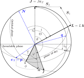
Figure 2: The geometry of the binary, having added the observer related frame $(\boldsymbol{p},\boldsymbol{q},\boldsymbol{N})$ (in dashed and dotted lines) with $\boldsymbol{N}$ as the line–of–sight vector, after removing the angles in the spin frame. The line–of–sight vector is chosen to lie in the $\boldsymbol{e}_{Y}$–$\boldsymbol{e}_{Z}$–plane, and measures an angle $i_{0}$ (associated with the rotation around $\boldsymbol{e_{X}}$) from $\boldsymbol{e_{Z}}$, such that $\boldsymbol{p}=\boldsymbol{e}_{X}$, and this is the point where the orbital plane meets the plane of the sky. Because of this rotation, the angle $i_{0}$ is also found between the vector $\boldsymbol{q}$, itself positioned in $(\boldsymbol{e_{Y}},\boldsymbol{e_{Z}})$, too, and $\boldsymbol{e_{Y}}$. The grey area in the graphics completely lies in the orbital plane, spanned by $(\boldsymbol{i},\boldsymbol{j})$ and $\varphi$ measures the angle between the separation vector $\boldsymbol{r}$ and $\boldsymbol{i}$. The polarization vectors $\boldsymbol{p}$ and $\boldsymbol{q}$ span the plane of the sky. The inclination of this plane with respect to the orbital plane is the orbital inclination $i$. The inclination of the orbital plane with respect to the invariable plane is denoted by $\Theta$. Please note that $\boldsymbol{L}$ does not lie on the unit sphere, only $\boldsymbol{k}$ does!

Inserting $p^{2}$ into Eq. (50), computing $p_{\phi}=\boldsymbol{p}\cdot\boldsymbol{e_{\phi}}$ and using the orthogonality relation of the used triad, one obtains

$$p_{r}^{2} =2E+\frac{2}{r}-\frac{L^{2}}{r^{2}}-\frac{2(\boldsymbol{L}\cdot\boldsymbol{S}_{\text{eff}})}{c^{2}r^{3}}\,,$$ (53a)

$$p_{\phi} =\frac{L_{z}}{r\sin\theta}\,,$$ (53b)

$$p_{\theta}^{2} =\frac{L^{2}}{r^{2}}-p_{\phi}^{2}=\frac{1}{r^{2}}\left(L^{2}-\frac{L_{z}^{2}}{\sin^{2}\theta}\right)\,,$$ (53c)

In KG05 , it was possible to reduce these equations by some algebraic relations and the fact that the angle $\Theta$ was constant in time - here, it is more complicated. It is still allowed to express $L_{z}$, the projection of $\boldsymbol{L}$ onto $\boldsymbol{e_{Z}}$, in Eq. (53b) and (53c) over $\Theta$ with the help of

$$p_{\phi} =\frac{L}{r}\frac{\cos\Theta}{\sin\theta}\,,$$ (54a)

$$p_{\theta}^{2} =\frac{L^{2}}{r^{2}}\left(1-\frac{\cos^{2}\Theta}{\sin^{2}\theta}\right)\,.$$ (54b)

Above equations are, for our purposes, the most simplified versions of the $p$ components and will enter in the dynamics of the angle $\varphi$ in their current form.

Our aim is now to connect the coordinate velocities, namely $\dot{r},\dot{\phi}$ and $\dot{\theta}$, to conserved quantities associated with the Hamiltonian of Eq. (50). Computation of the velocity in spherical coordinates, Eq. (51), gives following formulae using Hamilton’s EOM, $\dot{\boldsymbol{r}}=\partial{H}_{\text{NSO}}/\partial\boldsymbol{p}$, $\boldsymbol{n}\times\boldsymbol{e}_{\theta}=\boldsymbol{e}_{\phi}$ and $\boldsymbol{n}\times\boldsymbol{e}_{\phi}=-\boldsymbol{e}_{\theta}$.

$$\dot{r} =\boldsymbol{n}\cdot\dot{\boldsymbol{r}}=p_{r}\,,$$ (55a)

$$r\dot{\theta} =\boldsymbol{e}_{\theta}\cdot\dot{\boldsymbol{r}}=p_{\theta}+\frac{\boldsymbol{e}_{\phi}\cdot\boldsymbol{S}_{\text{eff}}}{c^{2}r^{2}}\,,$$ (55b)

$$r\sin\theta\dot{\phi} =\boldsymbol{e}_{\phi}\cdot\dot{\boldsymbol{r}}=p_{\phi}-\frac{\boldsymbol{e}_{\theta}\cdot\boldsymbol{S}_{\text{eff}}}{c^{2}r^{2}}\,.$$ (55c)

Of course, in the case of quasi-circular motion, $\dot{r}=0=p_{r}$ holds for all times. Remembering the geometry of Fig. 2, we recall that $\boldsymbol{r}$ is lying in the plane orthogonal to $\boldsymbol{L}$, which itself is spanned by the vectors $\boldsymbol{i}$ and $\boldsymbol{j}$. Calling $\varphi$ (the orbital phase) the measure for the angular distance from $\boldsymbol{i}$, we can write

$$\boldsymbol{r} =r\cos\varphi\,\boldsymbol{i}+r\sin\varphi\,\boldsymbol{j}\,.$$ (56)

The comparison of $\boldsymbol{r}$, given by Eqs. (52a) and (51), with the one in the new angular variables, Eq. (56) with Eqs. (14), implies the transformation

$$(\theta,\phi)\rightarrow(\Upsilon,\varphi):\begin{cases}\cos\theta=\sin\varphi\sin\Theta\\ \sin(\phi-\Upsilon)\sin\theta=\sin\varphi\cos\Theta\\ \cos(\phi-\Upsilon)\sin\theta=\cos\varphi\,.\end{cases}$$ (57)

Time derivation of the first equation will give an expression for $\dot{\theta}$, which can be simplified using the third one. The final expression is

$$\dot{\theta}=-\sin\Delta\,\dot{\Theta}-\sqrt{1-\frac{\cos^{2}\Theta}{\sin^{2}\theta}}\,\dot{\varphi}$$ (58)

with $\Delta\equiv\phi-\Upsilon$. Setting $\Theta$ constant, one naturally recovers Eq. (4.28a) of KG05 . Using this equation to eliminate $\dot{\theta}$ in (55b) and after substition $\pm p_{\theta}$ from (54b), one obtains a solution for $\dot{\varphi}$ and $\dot{\Upsilon}$

$$\dot{\varphi}={\mp}\frac{L}{r^{2}}-\frac{\tilde{S}_{\phi}}{\sqrt{1-\frac{\cos^{2}\Theta}{\sin^{2}\theta}}}\frac{1}{c^{2}\,r^{3}}-\frac{\sin\Delta}{\sqrt{1-\frac{\cos^{2}\Theta}{\sin^{2}\theta}}}\,\dot{\Theta}\,,$$ (59)

where $\tilde{S}_{\phi}$ is a shorthand for $\boldsymbol{S}_{\text{eff}}\cdot\boldsymbol{e_{\phi}}$. The ambiguity of the sign in the first term can be removed if one takes the rotation sense of the reduced mass, or equivalently, the direction of $\boldsymbol{L}$ into account. Having (initially) the vector $\boldsymbol{L}$ in the northern hemisphere, one should choose “$+$” in above equation. This condition then holds anytime as long as $S_{1}+S_{2}<\sqrt{L^{2}+J^{2}}$.

The quantity $L/r^{2}$ represents only the Newtonian point particle contribution. To express $r$ and $L$ in Eq. (59) in terms of $E$, one only needs Newtonian order,

$$r = (-2E)^{-1}\,,$$ (60)

$$L = (-2E)^{-1/2}\,.$$ (61)

Summarizing the evolution for $\dot{\varphi}$, one can separate it into a pure point particle (PP) and the spin orbit part (SO),

$$\dot{\varphi}=\dot{\varphi}_{\text{PP}}+\dot{\varphi}_{\text{SO}}\,.$$ (62)

The full 2PN expression for $\dot{\varphi}_{\text{PP}}$ can be extracted from Eqs.(5.6c), (5.6d) and (5.6k) of KG05 without spin dependent terms,

$$n =(-2E)^{3/2}\bigg{\{}1+\frac{(-2E)}{8c^{2}}\left(-15+\eta\right)+\frac{(-2E)^{2}}{128c^{4}}\biggl{[}555+30\eta+11\eta^{2}-\frac{192}{\sqrt{-2EL^{2}}}(5-2\eta)\biggr{]}\bigg{\}}\,,$$ (63a)

$$k =\frac{3}{c^{2}L^{2}}\biggl{\{}1+\frac{(-2E)}{4c^{2}}\left(-5+2\eta+\frac{35-10\eta}{-2EL^{2}}\right)\biggr{\}}\,,$$ (63b)

setting $e_{t}=0$ in

$$e_{t}^{2}= ~{}1+2EL^{2}+\frac{-2E}{4c^{2}}\bigg{\{}-8+8\eta+(17-7\eta)(-2EL^{2})-8\chi_{\text{so}}\cos\alpha\frac{S}{L}\bigg{\}}$$

$$~{}+\frac{(-2E)^{2}}{8c^{4}}\bigg{\{}8+4\eta+20\eta^{2}-(-2EL^{2})(112-47\eta+16\eta^{2})+24\sqrt{-2EL^{2}}(5-2\eta)$$

$$~{}+\frac{4}{(-2EL^{2})}\left(17-11\eta\right)-\frac{24}{\sqrt{-2EL^{2}}}\left(5-2\eta\right)\bigg{\}}$$ (64)

to eliminate $L$ and using $\dot{\varphi}_{\text{PP}}=n\,(1+k)$ DD85 , giving

$$\dot{\varphi}_{\text{PP}}= ~{}(-2E)^{3/2}\biggl{\{}1+{\frac{1}{8}}\left({9}+\eta\right)\frac{(-2E)}{c^{2}}+\biggl{[}{\frac{891}{128}}-{\frac{201}{64}}\,\eta+{\frac{11}{128}}\,{\eta}^{2}\biggr{]}\frac{{(-2E)}^{2}}{c^{4}}\biggr{\}}\,,$$ (65)

$$\dot{\varphi}_{\text{SO}}= ~{}{-3(\boldsymbol{k}\cdot\boldsymbol{S}_{\text{eff}}){(-2E)}^{3}+\frac{(-2E)^{3}\tilde{S}_{\phi}}{{\sqrt{1-\frac{\cos^{2}\Theta}{\sin^{2}\theta}}}}-\frac{\sin\Delta\dot{\Theta}}{{\sqrt{1-\frac{\cos^{2}\Theta}{\sin^{2}\theta}}}}\,,}$$ (66)

with

$$\tilde{S}_{\phi}\equiv ~{}\boldsymbol{S}_{\text{eff}}\cdot\boldsymbol{e}_{\phi}$$

$$= ~{}\cos(\phi-\Upsilon)[{S_{1}}\sin\phi_{s}\sin s(\delta_{1}-\delta_{2})\cos(\Theta-{\alpha_{\text{ks}}})-\sin(\Theta-{\alpha_{\text{ks}}})({S_{1}}\cos\tilde{s}(\delta_{1}-\delta_{2})+{S(\Theta)}\delta_{2})]$$

$$~{}+\sin(\phi-\Upsilon){S_{1}}\cos\phi_{s}\sin s(\delta_{2}-\delta_{1})\,.$$ (67)

The first term in $\dot{\varphi}_{SO}$, Eq. (66), comes from spin-orbit contributions to the value of $L$, as this is obtained from the energy expression (6), see section IV of KG05 . The angle $\phi$ can be computed with the help of Eq. (57) according to

$$\phi=\Upsilon+\arccos\left(\cos\varphi/\sqrt{1-\sin^{2}\varphi\sin^{2}\Theta}\right)\,.$$ (68)

Inserting the solutions $\Theta(t),\Upsilon(t)$ and $\phi_{s}(t)$ from sections IV and V to Eqs. (65) and (66), $\varphi$ can be obtained by numerical integration,

$$\varphi(t)=\int_{0}^{t}\dot{\varphi}\,\mbox{d}t+\varphi_{0}=\dot{\varphi}_{\text{PP}}\,t+\int_{0}^{t}\dot{\varphi}_{\text{SO}}(t)\,\mbox{d}t+\varphi_{0}\,.$$ (69)

The radial separation at 2PN accuracy, after eliminating L, reads

$$r= ~{}\frac{1}{(-2E)}\biggl{\{}1+\frac{(-2E)}{4c^{2}}\biggl{[}\eta-7+4\,{(\boldsymbol{k}\cdot\boldsymbol{S}_{\text{eff}})}\sqrt{(-2E)}\biggr{]}+\frac{(-2E)^{2}}{16c^{4}}\biggl{[}-67+\eta(54+\eta)\biggr{]}\biggr{\}}\,.$$ (70)

VII Gravitational waveforms

The gravitational wave polarization states, $h_{+}$ and $h_{\times}$, are usually given by

$$h_{+} =\frac{1}{2}\left(p_{i}p_{j}-q_{i}q_{j}\right)h_{ij}^{\text{TT}}\,,$$ (71a)

$$h_{\times} =\frac{1}{2}\left(p_{i}q_{j}+p_{j}q_{i}\right)h_{ij}^{\text{TT}}\,,$$ (71b)

where $p_{i}$ and $q_{i}$ are the components of the vectors $\boldsymbol{p}$ and $\boldsymbol{q}$ orthogonal to the observer’s direction, respectively, and $h_{ij}^{\text{TT}}$ is the transverse and traceless part of the radiation field $h_{ij}$. The leading order contribution, $h^{TT}_{ij}|_{Q}$, where the subscript $Q$ denotes quadrupolar approximation, reads WillWise96

$$h_{km}^{\text{TT}}\big{|}_{\text{Q}} =\frac{4G\mu}{c^{4}R^{\prime}}{\cal P}_{kmij}(\boldsymbol{N})\left(v_{ij}-\frac{GM}{r}n_{ij}\right)\,,$$ (72)

with ${\cal P}_{kmij}(\boldsymbol{N})$ as the usual transverse-traceless projection orthogonal to the line-of-sight vector $\boldsymbol{N}$, $R^{\prime}$ as the radial distance to the binary, the shorthands $v_{ij}\equiv v_{i}\,v_{j}$ and $n_{ij}\equiv n_{i}\,n_{j}$, using $\boldsymbol{v}\equiv d\boldsymbol{r}/dt$ as the velocity vector and $\boldsymbol{n}\equiv\boldsymbol{r}/r$ as the normalized relative separation, respectively.

Using Eq. (72), one may express both amplitudes of $h_{\times}$ and $h_{+}$ as

$$h_{+}\big{|}_{\text{Q}} =\frac{2G\mu}{c^{4}R^{\prime}}\left[\left(p_{i}p_{j}-q_{i}q_{j}\right)\left(v_{ij}-\frac{GM}{r}n_{ij}\right)\right]$$

$$=\frac{2G\mu}{c^{4}R^{\prime}}\bigg{\{}(\boldsymbol{p}\cdot\boldsymbol{v})^{2}-(\boldsymbol{q}\cdot\boldsymbol{v})^{2}$$

$$\quad-\frac{GM}{r}\left[(\boldsymbol{p}\cdot\boldsymbol{n})^{2}-(\boldsymbol{q}\cdot\boldsymbol{n})^{2}\right]\bigg{\}}\,,$$ (73a)

$$h_{\times}\big{|}_{\text{Q}} =\frac{2G\mu}{c^{4}R^{\prime}}\biggl{[}\left(p_{i}q_{j}+p_{j}q_{i}\right)\left(v_{ij}-\frac{GM}{r}n_{ij}\right)\biggr{]}$$

$$=\frac{4G\mu}{c^{4}R^{\prime}}\biggl{\{}(\boldsymbol{p}\cdot\boldsymbol{v})(\boldsymbol{q}\cdot\boldsymbol{v})-\frac{GM}{r}(\boldsymbol{p}\cdot\boldsymbol{n})(\boldsymbol{q}\cdot\boldsymbol{n})\biggr{\}}\,.$$ (73b)

To compute the two gravitational wave polarizations, one requires an expression for the radial separation vector $\boldsymbol{r}$ and its first time derivative. It is efficient to give $\boldsymbol{r}$ expanded in the observer’s triad $(\boldsymbol{p},\boldsymbol{q},\boldsymbol{N})$. In KG05 , this was done by expressing $\boldsymbol{r}$ in $(\boldsymbol{e_{X}},\boldsymbol{e_{Y}},\boldsymbol{e_{Z}})$ first, and secondly to compute this base from $(\boldsymbol{p},\boldsymbol{q},\boldsymbol{N})$ as rotated around $\boldsymbol{p}$ with the (constant) angle $i_{0}$. The result reads

$$\boldsymbol{r} =r\,\bigl{[}\left\{\cos\Upsilon\cos\varphi-C_{\Theta}\sin\Upsilon\sin\varphi\right\}\boldsymbol{p}$$

$$\quad+\left\{C_{i_{0}}\sin\Upsilon\cos\varphi-\left(S_{i_{0}}S_{\Theta}-C_{i_{0}}C_{\Theta}\cos\Upsilon\right)\sin\varphi\right\}\boldsymbol{q}$$

$$\quad+\left\{S_{i_{0}}\sin\Upsilon\cos\varphi+\left(C_{i_{0}}S_{\Theta}+S_{i_{0}}C_{\Theta}\cos\Upsilon\right)\sin\varphi\right\}\boldsymbol{N}\bigr{]}\,,$$ (74)

where $C_{i_{0}}$ and $S_{i_{0}}$ are shorthands for $\cos i_{0}$ and $\sin i_{0}$, respectively. The velocity vector $\boldsymbol{v}=d\boldsymbol{r}/dt$ is given by

$$\boldsymbol{v} = r\,\bigl{[}\bigl{\{}\dot{\Theta}\sin\Theta\sin\Upsilon\sin\varphi-\dot{\Upsilon}(\cos\Theta\cos\Upsilon\sin\varphi+\sin\Upsilon\cos\varphi)$$ (75)

$$-\dot{\varphi}(\cos\Theta\sin\Upsilon\cos\varphi+\cos\Upsilon\sin\varphi)\bigr{\}}\,\boldsymbol{p}$$

$$+\bigl{\{}\dot{\Theta}\sin\varphi(-(C_{i_{0}}\sin\Theta\cos\Upsilon+S_{i_{0}}\cos\Theta))+C_{i_{0}}\dot{\Upsilon}(\cos\Upsilon\cos\varphi-\cos\Theta\sin\Upsilon\sin\varphi)$$

$$+\dot{\varphi}(\cos\varphi(C_{i_{0}}\cos\Theta\cos\Upsilon-S_{i_{0}}\sin\Theta)-C_{i_{0}}\sin\Upsilon\sin\varphi)\bigr{\}}\,\boldsymbol{q}$$

$$+\bigl{\{}\dot{\Theta}\sin\varphi(C_{i_{0}}\cos\Theta-S_{i_{0}}\sin\Theta\cos\Upsilon)+S_{i_{0}}\dot{\Upsilon}(\cos\Upsilon\cos\varphi-\cos\Theta\sin\Upsilon\sin\varphi)$$

$$+\dot{\varphi}(\cos\varphi(S_{i_{0}}\cos\Theta\cos\Upsilon+C_{i_{0}}\sin\Theta)-S_{i_{0}}\sin\Upsilon\sin\varphi)\bigr{\}}\,\boldsymbol{N}\bigr{]}\,.$$

Having inserted above equations into (73), the final expressions for $h_{\times}$ and $h_{+}$ with time dependent $\Theta$ and the case of quasi-circular orbits are given by

$$h_{\times}|_{\text{Q}}^{[\dot{r}\equiv 0]}= \frac{2G\mu}{c^{4}R}\Bigl{\{}-\frac{Gm}{r}\bigl{[}(\cos\Upsilon\cos\varphi-\cos\Theta\sin\Upsilon\sin\varphi)(C_{i_{0}}(\cos\Theta\cos\Upsilon\sin\varphi+\sin\Upsilon\cos\varphi)$$ (76)

$$-S_{i_{0}}\sin\Theta\sin\varphi)\bigr{]}$$

$$+r^{2}\bigl{[}-\bigl{(}{\dot{\Theta}}\sin\Theta\sin\Upsilon\sin\varphi-{\dot{\Upsilon}}(\cos\Theta\cos\Upsilon\sin\varphi+\sin\Upsilon\cos\varphi)-{\dot{\varphi}}(\cos\Theta\sin\Upsilon\cos\varphi$$

$$+\cos\Upsilon\sin\varphi)\bigr{)}\bigr{]}\bigl{(}{\dot{\Theta}}\sin\varphi(C_{i_{0}}\sin(\Theta)\cos\Upsilon+S_{i_{0}}\cos\Theta)+C_{i_{0}}{\dot{\Upsilon}}(\cos\Theta\sin\Upsilon\sin\varphi$$

$$-\cos\Upsilon\cos\varphi)+{\dot{\varphi}}(-C_{i_{0}}\cos\Theta\cos\Upsilon\cos(\varphi)+S_{i_{0}}\sin\Theta\cos\varphi$$

$$+C_{i_{0}}\sin\Upsilon\sin\varphi)\bigr{)}\Bigr{\}}\,,$$

$${h_{+}}|_{\text{Q}}^{[\dot{r}\equiv 0]}= \frac{2G\mu}{c^{4}R}\biggl{\{}\frac{-Gm}{r}\bigl{[}(\cos\Upsilon\cos\varphi-\cos\Theta\sin\Upsilon\sin\varphi)^{2}-(\sin i_{0}\sin\Theta\sin\varphi$$ (77)

$$-C_{i_{0}}(\cos\Theta\cos\Upsilon\sin\varphi+\sin\Upsilon\cos\varphi))^{2}\bigr{]}$$

$$-r^{2}\bigl{[}{\dot{\Theta}}\sin\varphi(C_{i_{0}}\sin\Theta\cos\Upsilon+S_{i_{0}}\cos\Theta)+C_{i_{0}}{\dot{\Upsilon}}(\cos\Theta\sin\Upsilon\sin(\varphi)-\cos\Upsilon\cos\varphi)$$

$$+{\dot{\varphi}}(-C_{i_{0}}\cos\Theta\cos\Upsilon\cos\varphi+\sin i_{0}\sin\Theta\cos\varphi+C_{i_{0}}\sin\Upsilon\sin\varphi)\bigr{]}^{2}$$

$$+r^{2}\bigl{[}{\dot{\Theta}}(-\sin\Theta)\sin\Upsilon\sin\varphi+{\dot{\Upsilon}}(\cos\Theta\cos\Upsilon\sin\varphi+\sin\Upsilon\cos\varphi)$$

$$+{\dot{\varphi}}(\cos\Theta\sin\Upsilon\cos\varphi+\cos\Upsilon\sin\varphi)\bigr{]}^{2}\biggr{\}}\,.$$

VIII Conclusions and outlook

In this paper, the EOM of the spins and the orbital phase for the conservative 2PN accurate point particle were solved for the case of quasi-circular orbits, including the leading order spin-orbit interaction. The associated gravitational waveforms, $h_{+}$ and $h_{\times}$, in the quadrupolar restriction are given in analytic form. The spins are characterized by their constant magnitudes and 3 essential dynamic configuration angles, whose first order time derivatives were computed with the aid of Poisson brackets, and appear to decouple from the orbital phase. Although these equations are quite complicated and have to be integrated numerically in general, they reduce to quite simple ones in the case of equal masses and are then able to be solved exactly.

For small deviations from equal masses, a simple perturbative reduction scheme for the EOM can be employed. The associated first order corrections to the unperturbed equal-mass solution have been derived. The reliability of this solution naturally depends on the precision of measurement. The corrections are of the same PN order as the unperturbed solutions, multiplied by a factor of $F=(\delta_{1}-\delta_{2})/(\delta_{1}+\delta_{2})$. If we set $m_{2}~{}=~{}m_{1}\,(1~{}+~{}\alpha)$, we obtain following representative pairs $(\alpha,F(\alpha))$: (0.1, 0.04), (0.2, 0.08), (0.5, 0.17), (1.0, 0.29), to give an estimate of the magnitude of the perturbation. For the case of $\alpha<0.2$, this is below 10 $\%$, in other cases second-order perturbations may be required.

For a more complete representation, it will be highly demanded to include eccentricity (in progress) as well as higher-order spin dynamics, which have been found recently by Steinhoff et al. SSH08 ; SHS08 . Another important fact is that the radiation reaction (RR) has been neglected for this analysis. It will be a task to include the energy and angular momentum loss due to RR, which is under investigation.

IX Acknowledgments

I am grateful to thank Gerhard Schäfer for encouragement and carefully reading of the manuscript and Jan Steinhoff and Steven Hergt for helpful discussions. Special thanks are for Johannes Hartung for his crosschecks. This work was funded in part by the Deutsche Forschungsgemeinschaft (DFG) through SFB/TR7 “Gravitationswellenastronomie” and the DLR (Deutsches Zentrum für Luft- und Raumfahrt) through “LISA Germany”.

Appendix A solution of the full EOM by Lie series

For a consistency check, let us solve the problem perturbatively using the Lie series formalism GrLe_LIE and compare the results with the computation in the previous section. The idea is to associate a linear differential operator $\cal D$ to a system of differential equations and to apply this operator in an exponential series to the initial values. Successive computing of the addends will give the perturbed special solution to the required order. Let us suppose $\cal D$ to have the explicit form

$${\cal D}=\alpha_{1}(\boldsymbol{x})\frac{\partial}{\partial x_{1}}+...+\alpha_{n}(\boldsymbol{x})\frac{\partial}{\partial x_{n}}\,,$$ (78)

where $n$ is the number of independent variables and $\boldsymbol{x}=\{x_{i}\}$ with $i=(1,...,n)$. The $\alpha_{i}$ are functions of these variables. Then the operator ${\cal D}$, applied to the variable $x_{i}$, will give

$${\cal D}x_{i}=\alpha_{i}(\boldsymbol{x})\,.$$ (79)

Under certain assumptions (holomorphy of the $\alpha_{i}$), the series

$$e^{t\,{\cal D}}f(\boldsymbol{x})\equiv\sum_{\nu=0}^{\infty}\frac{t^{\nu}{\cal D}^{\nu}}{\nu!}f(\boldsymbol{x})=f(\boldsymbol{x})+t{\cal D}f(\boldsymbol{x})+\frac{t^{2}}{2!}{\cal D}^{2}f(\boldsymbol{x})...$$ (80)

converges absolutely and uniformly for some $|t|<T$. Defining $\boldsymbol{X}$ to be, in components,

$$X_{i}\equiv(e^{t\,{\cal D}}{x_{i}})\text{~{}with~{}}X_{i}|_{t=0}=x_{i}\,,$$ (81)

the following “exchange relation”

$$F(\boldsymbol{X})\equiv F(e^{t\,{\cal D}}\boldsymbol{x})=e^{t\,{\cal D}}F(\boldsymbol{x})$$ (82)

holds for the region of convergence. Computing the time derivative of the elements $X_{i}$, one can use the latter relation for the operator $\partial_{t}$ as the function $F$ and obtains

$$\frac{dX_{i}}{dt}=e^{t{\cal D}}[{\cal D}x_{i}]=e^{t{\cal D}}[\alpha_{i}(\boldsymbol{x})]=\alpha_{i}(\boldsymbol{X})\,.$$ (83)

This shows that the $X_{i}$ are solutions to Eq.. (83) in the region of convergence for the time $t$.

The next step is to split the operator ${\cal D}$ into one part ${\cal D}_{1}$, of which the solutions are exactly known, and another part ${\cal D}_{2}$ perturbing this system of differential equations, both supposed to be holomorpic functions in the same surrounding of the point $\boldsymbol{x}=\{x_{1},...x_{n}\}$. Let us define the solution to the operators ${\cal D}_{1}$ and ${\cal D}_{2}$ as

$$\boldsymbol{X}^{(0)}(t,\boldsymbol{x}) \equiv e^{t\,{\cal D}_{1}}\boldsymbol{x}\,,$$ (84)

$$\boldsymbol{X}(t,\boldsymbol{x}) \equiv e^{t\,{\cal D}}\boldsymbol{x}=e^{t\,({\cal D}_{1}+{\cal D}_{2})}\boldsymbol{x}\,.$$ (85)

Inside the region of convergence, the series for $\boldsymbol{X}$ can be resummed arbitrarily and cast into another more useful form

$$\boldsymbol{X}(t,\boldsymbol{x})= \boldsymbol{X^{(0)}}(t,\boldsymbol{x})$$

$$+\sum_{\nu=0}^{\infty}\int_{0}^{t}d\tau\frac{(t-\tau)^{\nu}}{\nu!}({\cal D}_{2}{\cal D}^{\nu}\boldsymbol{x})|_{\boldsymbol{x}=\boldsymbol{X^{(0)}}}\,.$$ (86)

The series runs over the label $\nu$ and the operator ${\cal D}_{2}{\cal D}^{\nu}$ has to be applied to $\boldsymbol{x}$ first, the unperturbed solution $\boldsymbol{g}(t,\boldsymbol{x})$ to be inserted afterwards, see GrLe_LIE for further information. The operator ${\cal D}_{2}$ can be shifted before the summation, which itself can also be exchanged with the integration, and what remains is

$$\boldsymbol{X}(t,\boldsymbol{x})=\boldsymbol{X}^{(0)}(t,\boldsymbol{x})+\int_{0}^{t}d\tau{\cal D}_{2}\boldsymbol{X}(t-\tau,\boldsymbol{x})|_{\boldsymbol{x}=\boldsymbol{X}^{(0)}(\tau,x)}\,.$$ (87)

This is an integral relation which can be solved iteratively. To any order, for example, the solution reads

$$\boldsymbol{X}^{(1)}(t,\boldsymbol{x})= ~{}\boldsymbol{X}^{(0)}(t,\boldsymbol{x})$$

$$~{}+\int_{0}^{t}[{{\cal D}_{2}}\boldsymbol{X}^{(0)}(t-\tau,\boldsymbol{x})]_{\boldsymbol{x}=\boldsymbol{X}^{(0)}(\tau,\boldsymbol{x})}]d\tau\,,~{}$$

$$\vdots$$

$$\boldsymbol{X}^{(\nu+1)}(t,\boldsymbol{x})= ~{}\boldsymbol{X}^{(0)}(t,\boldsymbol{x})$$

$$~{}+\int_{0}^{t}[{{\cal D}_{2}}\boldsymbol{X}^{(\nu)}(t-\tau,\boldsymbol{x})]_{\boldsymbol{x}=\boldsymbol{X}^{(0)}(\tau,\boldsymbol{x})}]d\tau\,.\hrulefill$$ (88)

For convergence issues, we note that this expression converges at least where the double series, Eq. (85), converges absolutely GR_LIE_appl . For a satisfying application of this algorithm, the operator ${\cal D}_{2}$ hast to be small; that means that the functions $\alpha_{i}^{(2)}(\boldsymbol{x})$ (the superscript 2 stands for the association to the second operator) are smaller in their magnitude in comparison to the coefficients $\alpha_{i}^{(1)}(\boldsymbol{x})$.

This algorithm applies excellently to the problem of a binary of arbitrarily configurated spins with unequal mass distribution, slightly deviating from the exact equal-mass case. The latter is already solved in KG05 , and what remains is to include perturbations. We will, for the time being, resort to the first order of the approximation scheme (A) to give a representative computation. Of course, the results will not sufficiently reflect the physics of the system after a long elapsed time and has to be expanded for further investigations.

To first-order in spin-orbit interactions, the motion of the spinning binary can be split into the equal mass spin-orbit evolution completed by the remainder built from the difference in the masses. Let us choose $\boldsymbol{X}=\{\Theta,\Upsilon,\phi_{s}\}$ as the functions to be evolved, then the EOM for $\boldsymbol{X}$, after the split, symbolically read

$$\dot{\Theta} =\chi_{1}\,{\cal T}_{1}(\Theta,\phi_{s})+\chi_{2}\,{\cal T}_{2}(\Theta,\phi_{s})\,,$$ (89a)

$$\dot{\Upsilon} =\chi_{1}\,{\cal U}_{1}(\Theta,\phi_{s})+\chi_{2}\,{\cal U}_{2}(\Theta,\phi_{s})\,,$$ (89b)

$$\dot{\phi}_{s} =\chi_{1}\,{\cal P}_{1}(\Theta,\phi_{s})+\chi_{2}\,{\cal P}_{2}(\Theta,\phi_{s})\,.$$ (89c)

The operators ${\cal D}_{1}$ and ${\cal D}_{2}$, therefore, read

$${\cal D}_{1} \equiv\chi_{1}\,\left({\cal T}_{1}\partial_{\Theta}+{\cal U}_{1}\partial_{\Upsilon}+{\cal P}_{1}\partial_{\phi_{s}}\right)\,,$$ (90)

$${\cal D}_{2} \equiv\chi_{2}\,\left({\cal T}_{2}\partial_{\Theta}+{\cal U}_{2}\partial_{\Upsilon}+{\cal P}_{2}\partial_{\phi_{s}}\right)\,.$$ (91)

For the full motion, Eqs. (89), then $\boldsymbol{X}(t)$ is given by the Lie series

$$\boldsymbol{X}(t)=e^{t\,({\cal D}_{1}+{\cal D}_{2})}\boldsymbol{X}(t=0)=e^{t\,({\cal D}_{1}+{\cal D}_{2})}\boldsymbol{x}\,.$$ (92)

The relation for the perturbative functions can be computed using the unperturbed one, associated with the equal-mass case. The generic angles therein, $\boldsymbol{X^{(0)}}~{}=~{}\{\Theta^{(0)},\Upsilon^{(0)},\phi_{s}^{(0)}\}$, read

$$\Upsilon^{(0)}(t) = \Omega_{\Upsilon}\,t\,+\Upsilon_{0}\,,$$ (93)

$$\phi_{s}^{(0)}(t) = \Omega_{\phi_{s}}\,t\,+{\phi_{s}}_{0}\,,$$ (94)

$$\Theta^{(0)}(t) = \Theta_{0}\,,$$ (95)

with constant angular velocities, given by Eqs. (30). The first order solutions formally read

$${\Theta}^{(1)}(t)-{\Theta^{(0)}}(t) =\int_{0}^{t}\left\{{\cal D}_{2}\,{\Theta^{(0)}}(t-\tau,\boldsymbol{x})\right\}_{\boldsymbol{x}=\boldsymbol{X}^{(0)}(\tau,\boldsymbol{x})}d\tau\,,$$ (96a)

$${\Upsilon}^{(1)}(t)-{\Upsilon^{(0)}}(t) =\int_{0}^{t}\left\{{\cal D}_{2}\,{\Upsilon^{(0)}}(t-\tau,\boldsymbol{x})\right\}_{\boldsymbol{x}=\boldsymbol{X}^{(0)}(\tau,\boldsymbol{x})}d\tau\,,$$ (96b)

$${\phi_{s}}^{(1)}(t)-{\phi_{s}^{(0)}}(t) =\int_{0}^{t}\left\{{\cal D}_{2}\,{\phi_{s}^{(0)}}(t-\tau,\boldsymbol{x})\right\}_{\boldsymbol{x}=\boldsymbol{X}^{(0)}(\tau,\boldsymbol{x})}d\tau\,.~{}~{}~{}~{}~{}~{}~{}~{}~{}$$ (96c)

All perturbing functions, computed by Eqs. (96), are in complete agreement with the ones in section V.

References

(1)
T. Damour, B. R. Iyer, and B.S. Sathyaprakash, Phys. Rev. D 63, 044023 (2001)
(2)
G. Schäfer and N. Wex,
Phys. Lett. A 174, 196 (1993).
Erratum: Phys. Lett. A 177, 461 (1993)
(3)
T. Damour, A. Gopakumar, and B. R. Iyer,
Phys. Rev. D 70, 064028 (2004)
(4)
N. Yunes, K. Arun, E. Berti, and C. Will,
Post-Circular Expansion of Eccentric Binary Inspirals: Fourier-Domain Waveforms in the Stationary Phase Approximation,
arXiv:gr-qc/0906.0313v1
(5)
L. E. Kidder, C. M. Will, and A. G. Wiseman,
Phys. Rev. D 47, R4183 (1993)
(6)
C. Cutler and E. E. Flanagan
Phys. Rev. D 49, 2658 (1994)
(7)
A. Buonanno, Y. Chen, and M. Vallisneri,
Phys. Rev. D, 67, 104025 (2003)
(8)
A. Buonanno, Y. Chen, Y. Pan, H. Tagoshi, and M. Vallisneri,
Phys. Rev. D 72, 084027 (2005)
(9)
T. A. Apostolatos,
Phys. Rev. D 52, 605 (1995)
(10)
A. Papapetrou,
Proc. R. Soc. Lond. A, 209, 248 (1951)
(11)
G. Faye, L. Blanchet, and A. Buonanno
Phys. Rev. D 74, 104033 (2006)
(12)
L. Blanchet, A. Buonanno, and G. Faye,
Phys. Rev. D 74, 104034 (2006)
(13)
R. Arnowitt, S. Deser, and C. W. Misner, in Gravitation: An Introduction to Current Research,
edited by L. Witten (Wiley, New York 1962), p. 227, arXiv:gr-qc/0405109
(14)
T. Damour, P. Jaranowski, and G. Schäfer,
Phys. Rev. D 77, 064032 (2008)
(15)
J. Steinhoff, G. Schäfer, and S. Hergt,
Phys. Rev. D 77, 104018 (2008)
(16)
J. Steinhoff, S. Hergt, and G. Schäfer,
Phys. Rev. D 78, 101503(R) (2008)
(17)
T. Damour, P. Jaranowski, and G. Schäfer,
Phys. Lett. B 513, 147 (2001)
(18)
C. Königsdörffer and A. Gopakumar,
Phys. Rev. D 71, 024039 (2005)
(19)
P. Jaranowski and G. Schäfer,
Ann. Phys. 9, 378 (2000)
(20)
B. M. Barker and R. F. O’Connell, Phys. Rev D 2, 1428 (1970)
(21)
T. Damour and G. Schäfer,
Nuovo Cimento, 101B, 127 (1988)
(22)
T. Damour and N. Deruelle, Ann. Inst. Henri Poincaré Phys. Theor. 43, 107 (1985)
(23)
C. M. Will and A. G. Wiseman,
Phys. Rev. D 54, 4813 (1996)
(24)
W. Gröbner and P. Lesky, Mathematische Methoden der Physik II (Bibliographisches Institut AG,
Mannheim, 1965)
(25)
W. Gröbner, Die Lie-Reihen und ihre Anwendungen (VEB Deutscher Verlag der Wissenschaft,
Berlin, 1960)
(26)
R. M. Memmesheimer, A. Gopakumar, and G. Schäfer, Phys. Rev. D 70, 104011 (2004)
(27)
T. Damour, P. Jaranowski, and G. Schäfer,
Phys. Rev. D, 78, 024009 (2008)
(28)
T. Damour, P. Jaranowski, and G. Schäfer,
Phys. Rev. D 62, 021501(R) (2000)