Coupling Conditions for the $3\times 3$ Euler System

Abstract

This paper is devoted to the extension to the full $3\times 3$ Euler system of the basic analytical properties of the equations governing a fluid flowing in a duct with varying section. First, we consider the Cauchy problem for a pipeline consisting of 2 ducts joined at a junction. Then, this result is extended to more complex pipes. A key assumption in these theorems is the boundedness of the total variation of the pipe’s section. We provide explicit examples to show that this bound is necessary.

Keywords: Conservation Laws at Junctions, Coupling Conditions at Junctions.

2000 MSC: 35L65, 76N10

1 Introduction

We consider Euler equations for the evolution of a fluid flowing in a pipe with varying section $a=a(x)$, see [17, Section 8.1] or [12, 15]:

$$\left\{\begin{array}[]{ll}\displaystyle\partial_{t}(a\rho)+\partial_{x}(aq)=0\\ \displaystyle\partial_{t}(aq)+\partial_{x}\left[aP\left(\rho,q,E\right)\right]=p\left(\rho,e\right)\,\partial_{x}a\\ \displaystyle\partial_{t}(aE)+\partial_{x}\left[aF\left(\rho,q,E\right)\right]=0\end{array}\right.$$ (1.1)

where, as usual, $\rho$ is the fluid density, $q$ is the linear momentum density and $E$ is the total energy density. Moreover

$$\!\!\!E(\rho,q,E)=\frac{1}{2}\frac{q^{2}}{\rho}+\rho e,\quad P(\rho,q,E)=\frac{q^{2}}{\rho}+p,\quad F(\rho,q,E)=\frac{q}{\rho}(E+p)\,,$$ (1.2)

with $e$ being the internal energy density, $P$ the flow of the linear momentum density and $F$ the flow of the energy density. The above equations express the conservation laws for the mass, momentum, and total energy of the fluid through the pipe. Below, we will often refer to the standard case of the ideal gas, characterized by the relations

$$p=(\gamma-1)\rho e,\qquad S=\ln e-(\gamma-1)\ln\rho\,,$$ (1.3)

for a suitable $\gamma>1$. Note however, that this particular equation of state is necessary only in case (p) of Proposition 3.1 and has been used in the examples in Section 4. In the rest of this work, the usual hypothesis [16, formula (18.8)], that is $p>0$, $\partial_{\tau}p(\tau,S)<0$ and $\partial^{2}_{\tau\tau}p(\tau,S)>0$, are sufficient.

The case of a sharp discontinuous change in the pipe’s section due to a junction sited at, say, $x=0$, corresponds to $a(x)=a^{-}$ for $x<0$ and $a(x)=a^{+}$ for $x>0$. Then, the motion of the fluid can be described by

$$\left\{\begin{array}[]{ll}\displaystyle\partial_{t}\rho+\partial_{x}q=0\\ \displaystyle\partial_{t}q+\partial_{x}P(\rho,q,E)=0\\ \displaystyle\partial_{t}E+\partial_{x}F(\rho,q,E)=0,\end{array}\right.$$ (1.4)

for $x\neq 0$, together with a coupling condition at the junction of the form:

$$\Psi\left(a^{-},(\rho,q,E)(t,0-);a^{+},(\rho,q,E)(t,0+)\right)=0.$$ (1.5)

Above, we require the existence of the traces at $x=0$ of $(\rho,q,E)$. Various choices of the function $\Psi$ are present in the literature, see for instance [1, 5, 8, 9] in the case of the $p$-system and [10] for the full $3\times 3$ system (1.4). Here, we consider the case of a general coupling condition which comprises all the cases found in the literature. Within this setting, we prove the well posedness of the Cauchy problem for (1.4)–(1.5). Once this result is obtained, the extension to pipes with several junctions and to pipes with a $\mathbf{W^{1,1}}$ section is achieved by the standard methods considered in the literature. For the analytical techniques to cope with networks having more complex geometry, we refer to [11].

The above statements are global in time and local in the space of the thermodynamic variables $(\rho,q,E)$. Indeed, for any fixed (subsonic) state $(\bar{\rho},\bar{q},\bar{E})$, there exists a bound on the total variation $\mathrm{TV}(a)$ of the pipe’s section, such that all sections below this bound give rise to Cauchy problems for (1.4)–(1.5) that are well posed in $\mathbf{L^{1}}$. We show the necessity of this bound in the conditions found in the current literature. Indeed, we provide explicit examples showing that a wave can be arbitrarily amplified through consecutive interactions with the pipe walls, see Figure 1.

The paper is organized as follows. The next section is divided into three parts, the former one deals with a single junction and two pipes, then we consider $n$ junctions and $n+1$ pipes, the latter part presents the case of a $\mathbf{W^{1,1}}$ section. Section 3 is devoted to different specific choices of coupling conditions (1.5). In Section 4, an explicit example shows the necessity of the bound on the total variation of the pipe’s section. All proofs are gathered in Section 5.

2 Basic Well Posedness Results

Throughout, we let $u=(\rho,q,E)$. We denote by ${\mathbb{R}}^{+}$ the real halfline $\left[0,+\infty\right[$, while $\mathaccent 23{{\mathbb{R}}}^{+}=\left]0,+\infty\right[$. Following various results in the literature, such as [1, 2, 5, 8, 9, 10, 13], we limit the analysis in this paper to the subsonic region given by $\lambda_{1}(u)<0<\lambda_{3}(u)$ and $\lambda_{2}(u)\neq 0$, where $\lambda_{i}$ is the $i-$th eigenvalue of (1.4), see (5.1). Without any loss of generality, we further restrict to

$$A_{0}=\left\{u\in\mathaccent 23{{\mathbb{R}}}^{+}\times{\mathbb{R}}^{+}\times\mathaccent 23{{\mathbb{R}}}^{+}\colon\lambda_{1}(u)<0<\lambda_{2}(u)\right\}\,.$$ (2.6)

Note that we fix a priori the sign of the fluid speed $v$, since $\lambda_{2}(u)=q/\rho=v>0$.

2.1 A Junction and two Pipes

We now give the definition of weak $\Psi-$solution to the Cauchy Problem for (1.4) equipped with the condition (1.5), extending [5, Definition 2.1] and [9, Definition 2.2] to the $3\times 3$ case (1.4) and comprising the particular case covered in [10, Definition 2.4].

Definition 2.1

Let $\Psi\colon(\mathaccent 23{{\mathbb{R}}}^{+}\times A_{0})^{2}\to{\mathbb{R}}^{3}$, $u_{o}\in\mathbf{BV}({\mathbb{R}};A_{0})$ and two positive sections $a^{-}$, $a^{+}$ be given. A $\Psi$-solution to (1.4) with initial datum $u_{o}$ is a map

$$\begin{array}[]{rcl}u&\in&\mathbf{C^{0}}\left({\mathbb{R}}^{+};\mathbf{L^{1}_{loc}}({\mathbb{R}}^{+};A_{0})\right)\\ u(t)&\in&\mathbf{BV}({\mathbb{R}};A_{0})\quad\mbox{ for a.e. }t\in{\mathbb{R}}^{+}\end{array}$$ (2.7)

such that

1.

for $x\neq 0$, $u$ is a weak entropy solution to (1.4);

2.

for a.e. $x\in{\mathbb{R}}$, $u(0,x)=u_{o}(x)$;

3.

for a.e. $t\in{\mathbb{R}}^{+}$, the coupling condition (1.5) at the junction is met.

Below, extending the $2\times 2$ case of the $p$-system, see [1, 4, 5, 8, 9], we consider some properties of the coupling condition (1.5), which we rewrite here as

$$\Psi(a^{-},u^{-};a^{+},u^{+})=0\,.$$ (2.8)

($\mathbf{\Psi}$0)

Regularity: $\Psi\in\mathbf{C^{1}}\left((\mathaccent 23{{\mathbb{R}}}^{+}\times A_{0})^{2};{\mathbb{R}}^{3}\right)$.

($\mathbf{\Psi}$1)

No-junction case: for all $a>0$ and all $u^{-},u^{+}\in A_{0}$, then

$$\Psi(a,u^{-};a,u^{+})=0\Longleftrightarrow u^{-}=u^{+}\,.$$

($\mathbf{\Psi}$2)

Consistency: for all positive $a^{-},a^{0},a^{+}$ and all $u^{-},u^{0},u^{+}\in A_{0}$,

$$\begin{array}[]{l}\Psi(a^{-},u^{-};a^{0},u^{0})=0\\ \Psi(a^{0},u^{0};a^{+},u^{+})=0\end{array}\Longrightarrow\Psi(a^{-},u^{-};a^{+},u^{+})=0\,.$$

Moreover, by an immediate extension of [9, Lemma 2.1], ($\mathbf{\Psi 0}$) ensures that (2.8) implicitly defines a map

$$u^{+}=T(a^{-},a^{+};u^{-})$$ (2.9)

in a neighborhood of any pair of subsonic states $u^{-}$, $u^{+}$ and sections $a^{-},a^{+}$ that satisfy $\Psi(a^{-},u^{-};a^{+},u^{+})=0$.

The technique in [6] allows to prove the following well posedness result.

Theorem 2.2

Assume that $\Psi$ satisfies conditions ($\mathbf{\Psi}$0)-($\mathbf{\Psi}$2). For every $\bar{a}>0$ and $\bar{u}\in A_{0}$ such that

$$\det\left[D_{u^{-}}\Psi\cdot r_{1}(\bar{u})\quad D_{u^{+}}\Psi\cdot r_{2}(\bar{u})\quad D_{u^{+}}\Psi\cdot r_{3}(\bar{u})\right]\neq 0$$ (2.10)

there exist positive $\delta$, $L$ such that for all $a^{-},a^{+}$ with ${\left|a^{+}-\bar{a}\right|}+{\left|a^{-}-\bar{a}\right|}<\delta$ there exists a semigroup $S\colon{\mathbb{R}}^{+}\times\mathcal{D}\to\mathcal{D}$ with the following properties:

1. $\mathcal{D}\supseteq\left\{u\in\bar{u}+\mathbf{L^{1}}({\mathbb{R}};A_{0})\colon\mathrm{TV}(u)<\delta\right\}$.

2. For all $u\in\mathcal{D}$, $S_{0}u=u$ and for all $t,s\geq 0$, $S_{t}S_{s}u=S_{s+t}u$.

3. For all $u,u^{\prime}\in\mathcal{D}$ and for all $t,t^{\prime}\geq 0$,

   $${\left\|S_{t}u-S_{t^{\prime}}u^{\prime}\right\|}_{\mathbf{L^{1}}}\leq L\cdot\left({\left\|u-u^{\prime}\right\|}_{\mathbf{L^{1}}}+{\left|t-t^{\prime}\right|}\right)$$

4. If $u\in\mathcal{D}$ is piecewise constant, then for $t$ small, $S_{t}u$ is the gluing of solutions to Riemann problems at the points of jump in $u$ and at the junction at $x=0$.

5. For all $u_{o}\in\mathcal{D}$, the orbit $t\to S_{t}u_{o}$ is a $\Psi$-solution to (1.4) with initial datum $u_{o}$.

The proof is postponed to Section 5. Above $r_{i}(u)$, with $i=1,2,3$, are the right eigenvectors of $Df(u)$, see (5.1). Moreover, by solution to the Riemann Problems at the points of jump we mean the usual Lax solution, see [3, Chapter 5], whereas for the definition of solution to the Riemann Problems at the junction we refer to [8, Definition 2.1].

2.2 $n$ Junctions and $n+1$ Pipes

The same procedure used in [9, Paragraph 2.2] allows now to construct the semigroup generated by (1.4) in the case of a pipe with piecewise constant section

$$a=a_{0}\,\chi_{]-\infty,x_{1}]}+\sum_{j=1}^{n-1}a_{j}\,\chi_{[x_{j},x_{j+1}[}+a_{n}\,\chi_{[x_{n},+\infty[}$$

with $n\in{\mathbb{N}}$. In each segment $\left]x_{j},x_{j+1}\right[$, the fluid is modeled by (1.4). At each junction $x_{j}$, we require condition (1.5), namely

$$\Psi(a_{j-1},u_{j}^{-};a_{j},u_{j}^{+})=0\quad\begin{array}[]{l}\mbox{ for all }j=1,\ldots,n\mbox{, where}\\ \displaystyle u_{j}^{\pm}=\lim_{x\to x_{j}\pm}u_{j}(x)\,.\end{array}$$ (2.11)

We omit the formal definition of $\Psi$-solution to (1.4)–(1.5) in the present case, since it is an obvious iteration of Definition 2.1. The natural extension of Theorem 2.2 to the case of (1.4)–(2.11) is the following result.

Theorem 2.3

Assume that $\Psi$ satisfies conditions ($\mathbf{\Psi}$0)-($\mathbf{\Psi}$2). For any $\bar{a}>0$ and any $\bar{u}\in A_{0}$, there exist positive $M,\Delta,\delta,L,\mathcal{M}$ such that for any pipe’s profile satisfying

$$a\in\mathbf{PC}\left({\mathbb{R}};\left]\bar{a}-\Delta,\bar{a}+\Delta\right[\right)\mbox{ with }\mathrm{TV}(a)<M$$ (2.12)

there exists a piecewise constant stationary solution

$$\hat{u}=\hat{u}_{0}\chi_{\left]-\infty,x_{1}\right[}+\sum_{j=1}^{n-1}\hat{u}_{j}\chi_{\left]x_{j},x_{j+1}\right[}+\hat{u}_{n}\chi_{\left]x_{n},+\infty\right[}$$

to (1.4)–(2.11) satisfying

$$\hat{u}_{j}\in A_{0}\mbox{ with }{\left|\hat{u}_{j}-\bar{u}\right|}<\delta\mbox{ for }j=0,\ldots n$$

$$\Psi\left(a_{j-1},\hat{u}_{j-1};a_{j},\hat{u}_{j}\right)=0\mbox{ for }j=1,\ldots,n$$

$$\mathrm{TV}(\hat{u})\leq\mathcal{M}\,\mathrm{TV}(a)$$ (2.13)

and a semigroup $S^{a}\colon{\mathbb{R}}^{+}\times\mathcal{D}^{a}\to\mathcal{D}^{a}$ such that

1. $\mathcal{D}^{a}\supseteq\left\{u\in\hat{u}+\mathbf{L^{1}}({\mathbb{R}};A_{0})\colon\mathrm{TV}(u-\hat{u})<\delta\right\}$.

2. $S^{a}_{0}$ is the identity and for all $t,s\geq 0$, $S^{a}_{t}S^{a}_{s}=S^{a}_{s+t}$.

3. For all $u,u^{\prime}\in\mathcal{D}^{a}$ and for all $t,t^{\prime}\geq 0$,

   $${\left\|S^{a}_{t}u-S^{a}_{t^{\prime}}u^{\prime}\right\|}_{\mathbf{L^{1}}}\leq L\cdot\left({\left\|(u)-u^{\prime}\right\|}_{\mathbf{L^{1}}}+{\left|t-t^{\prime}\right|}\right).$$

4. If $u\in\mathcal{D}^{a}$ is piecewise constant, then for $t$ small, $S_{t}u$ is the gluing of solutions to Riemann problems at the points of jump in $u$ and at each junction $x_{j}$.

5. For all $u\in\mathcal{D}^{a}$, the orbit $t\to S^{a}_{t}u$ is a weak $\Psi$-solution to (1.4)–(2.11).

We omit the proof, since it is based on the natural extension to the present $3\times 3$ case of [9, Theorem 2.4]. Remark that, as in that case, $\delta$ and $L$ depend on $a$ only through $\bar{a}$ and $\mathrm{TV}(a)$. In particular, all the construction above is independent from the number of points of jump in $a$.

2.3 A Pipe with a $\mathbf{W^{1,1}}$ Section

In this paragraph, the pipe’s section $a$ is assumed to satisfy

$$\left\{\begin{array}[]{l}a\in\mathbf{W^{1,1}}\left({\mathbb{R}};\left]\bar{a}-\Delta,\bar{a}+\Delta\right[\right)\mbox{ for suitable }\Delta>0,\ \bar{a}>\Delta\\ \mathrm{TV}(a)<M\mbox{ for a suitable }M>0\\ a^{\prime}(x)=0\mbox{ for a.e. }x\in{\mathbb{R}}\setminus[-X,X]\mbox{ for a suitable }X>0\,.\end{array}\right.\!\!$$ (2.14)

The same procedure used in [9, Theorem 2.8] allows to construct the semigroup generated by (1.1) in the case of a pipe which satisfies (2.14). Indeed, thanks to Theorem 2.3, we approximate $a$ with a piecewise constant function $a_{n}$. The corresponding problems to (1.4)–(2.11) generate semigroups $S_{n}$ defined on domains characterized by uniform bounds on the total variation and that are uniformly Lipschitz in time. Here, uniform means also independent from the number of junctions. Therefore, we prove the pointwise convergence of the $S_{n}$ to a limit semigroup $S$, along the same lines in [9, Theorem 2.8].

3 Coupling Conditions

This section is devoted to different specific choices of (2.8).

(S)-Solutions

We consider first the coupling condition inherited from the smooth case. For smooth solutions and pipes’ sections, system (1.1) is equivalent to the $3\times 3$ balance law

$$\left\{\begin{array}[]{ll}\displaystyle\partial_{t}\rho+\partial_{x}q=-\frac{q}{a}\,\partial_{x}a\\ \displaystyle\partial_{t}q+\partial_{x}P(\rho,q,E)=-\frac{q^{2}}{a\rho}\,\partial_{x}a\\ \displaystyle\partial_{t}E+\partial_{x}F(\rho,q,E)=-\frac{F}{a}\,\partial_{x}a.\end{array}\right.$$ (3.1)

The stationary solutions to (1.1) are characterized as solutions to

$$\!\!\!\left\{\!\!\!\!\begin{array}[]{ll}\partial_{x}(a(x)\,q)=0\\ \partial_{x}\!\left(a(x)\,P(\rho,q,E)\right)=p(\rho,e)\,\partial_{x}a\\ \partial_{x}\!\left(a(x)\,F(\rho,q,E)\right)=0\end{array}\right.\mbox{ or }\left\{\!\!\!\!\begin{array}[]{ll}\partial_{x}q=-\frac{q}{a}\,\partial_{x}a\\ \partial_{x}P\left(\rho,q,E\right)=-\frac{q^{2}}{a\rho}\,\partial_{x}a\\ \partial_{x}F\left(\rho,q,E\right)=-\frac{F}{a}\,\partial_{x}a\,.\end{array}\right.\!\!\!$$ (3.2)

As in the $2\times 2$ case of the $p$-system, the smoothness of the sections induces a unique choice for condition (2.8), see [9, (2.3) and (2.19)], which reads

$$\mbox{{(S)}}\quad\Psi=\left[\!\!\!\begin{array}[]{l}a^{+}q^{+}-a^{-}q^{-}\\ \displaystyle a^{+}P(u^{+})-a^{-}P(u^{-})+\int_{-X}^{X}p\left(\mathcal{R}^{a}(x),\mathcal{E}^{a}(x)\right)a^{\prime}(x)\mathrm{d}x\!\\ a^{+}F(u^{+})-a^{-}F(u^{-})\end{array}\!\right]$$ (3.3)

where $a=a(x)$ is a smooth monotone function satisfying $a(-X)=a^{-}$ and $a(X)=a^{+}$, for a suitable $X>0$. $\mathcal{R}^{a},\mathcal{E}^{a}$ are the $\rho$ and $e$ component in the solution to (3.2) with initial datum $u^{-}$ assigned at $-X$. Note that, by the particular form of (3.3), the function $\Psi$ is independent both from the choice of $X$ and from that of the map $a$, see [9, 2. in Proposition 2.7].

(P)-Solutions

The particular choice of the coupling condition in [10, Section 3] can be recovered in the present setting. Indeed, conditions (M), (E) and (P) therein amount to the choice

$$\mbox{{(P)}}\qquad\Psi(a^{-},u^{-},a^{+},u^{+})=\left[\begin{array}[]{c}a^{+}q^{+}-a^{-}q^{-}\\ P(u^{+})-P(u^{-})\\ a^{+}F(u^{+})-a^{-}F(u^{-})\end{array}\right],$$ (3.4)

where $a^{+}$ and $a^{-}$ are the pipe’s sections. Consider fluid flowing in a horizontal pipe with an elbow or kink, see [14]. Then, it is natural to assume the conservation of the total linear momentum along directions dependent upon the geometry of the elbow. As the angle of the elbow vanishes, one obtains the condition above, see [10, Proposition 2.6].

(L)-Solutions

We can extend the construction in [1, 2, 4] to the $3\times 3$ case (1.4). Indeed, the conservation of the mass and linear momentum in [4] with the conservation of the total energy for the third component lead to the choice

$$\mbox{{(L)}}\qquad\Psi(a^{-},u^{-},a^{+},u^{+})=\left[\begin{array}[]{c}a^{+}q^{+}-a^{-}q^{-}\\ a^{+}P(u^{+})-a^{-}P(u^{-})\\ a^{+}F(u^{+})-a^{-}F(u^{-})\end{array}\right],$$ (3.5)

where $a^{+}$ and $a^{-}$ are the pipe’s sections. The above is the most immediate extension of the standard definition of Lax solution to the case of the Riemann problem at a junction.

(p)-Solutions

Following [1, 2], motivated by the what happens at the hydrostatic equilibrium, we consider a coupling condition with the conservation of the pressure $p(\rho)$ in the second component of $\Psi$. Thus

$$\mbox{{(p)}}\qquad\Psi(a^{-},u^{-},a^{+},u^{+})=\left[\begin{array}[]{c}a^{+}\,q^{+}-a^{-}\,q^{-}\\ p(\rho^{+},e^{+})-p(\rho^{-},e^{-})\\ a^{+}F(u^{+})-a^{-}F(u^{-})\end{array}\right],$$ (3.6)

where $a^{+}$ and $a^{-}$ are the pipe’s sections.

Proposition 3.1

For every $\bar{a}>0$ and $\bar{u}\in A_{0}$, each of the coupling conditions $\Psi$ in (3.3), (3.4), (3.5), (3.6) satisfies the requirements ($\mathbf{\Psi}$0)-($\mathbf{\Psi}$2) and (2.10). In the case of (3.6), we also require that the fluid is perfect, i.e. that (1.3) holds.

The proof is postponed to Section 5. Thus, Theorem 2.2 applies, yielding the well posedness of (1.4)–(1.5) with each of the particular choices of $\Psi$ in (3.3), (3.4), (3.5), (3.6).

4 Blow-Up of the Total Variation

In the previous results a key role is played by the bound on the total variation $\mathrm{TV}(a)$ of the pipe’s section. This requirement is intrinsic to problem (1.4)–(1.5) and not due to the technique adopted above. Indeed, we show below that in each of the cases (3.3), (3.4), (3.5), (3.6), it is possible to choose an initial datum and a section $a\in\mathbf{BV}({\mathbb{R}};[a^{-},a^{+}])$ with $a^{+}-a^{-}$ arbitrarily small, such that the total variation of the corresponding solution to (1.4)–(1.5) becomes arbitrarily large.

Consider the case in Figure 1.

\psfrag{a}{$x$}\psfrag{e}{$\Delta a$}\psfrag{b}{$a$}\psfrag{c}{$x$}\psfrag{f}{$\sigma_{3}^{-}$}\psfrag{g}{$\sigma_{3}^{+}$}\psfrag{h}{$\sigma_{3}^{++}$}\psfrag{d}{$t$}\psfrag{l}{$u^{+}$}\psfrag{i}{$u$}\psfrag{n}{$2l$}\psfrag{m}{$l$}\includegraphics[width=170.71652pt]{f.eps}

Figure 1: A wave $\sigma_{3}^{-}$ hits a junction where the pipe’s section increases by $\Delta a$. From this interaction, the wave $\sigma_{3}^{+}$ arises, which hits a second junction, where the pipe section decreases by $\Delta a$.

A wave $\sigma_{3}^{-}$ hits a junction where the pipe’s section increases by, say, $\Delta a>0$. The fastest wave arising from this interaction is $\sigma_{3}^{+}$, which hits the second junction where the section diminishes by $\Delta a$.

Solving the Riemann problem at the first interaction amounts to solve the system

$$L_{3}\left(L_{2}\left(T\left(L_{1}(u;\sigma_{1}^{+})\right);\sigma_{2}^{+}\right);\sigma_{3}^{+}\right)=T\left(L_{3}(u;\sigma_{3}^{-})\right),$$ (4.1)

where $u\in A_{0}$, see Figure 2 for the definitions of the waves’ strengths $\sigma_{i}^{+}$ and $\sigma_{3}^{-}$. Above, $T$ is the map defined in (2.9), which in turn depends from the specific condition (2.8) chosen. In the expansions below, we use the $(\rho,q,e)$ variables, thus setting $u=(\rho,q,e)$ throughout this section.

\psfrag{s3m}{$\!\!\!\!\sigma_{3}^{-}$}\psfrag{s1p}{$\sigma_{1}^{+}$}\psfrag{s2p}{$\sigma_{2}^{+}$}\psfrag{s3p}{$\sigma_{3}^{+}$}\psfrag{1}{$u$}\psfrag{2}{}\psfrag{3}{}\psfrag{4}{$u^{+}$}\psfrag{5}{}\psfrag{6}{}\includegraphics[width=113.81102pt]{NotInter.eps}

Figure 2: Notation used in (4.1) and (4.4).

Differently from the case of the $2\times 2$ $p$-system in [9], here we need to consider the second order expansion in $\Delta a=a^{+}-a^{-}$ of the map $T$; that is

$$T(a,a+\Delta a;u)=u+H(u)\frac{\Delta a}{a}+G(u)\left(\frac{\Delta a}{a}\right)^{2}+o\left(\frac{\Delta a}{a}\right)^{2}$$ (4.2)

The explicit expressions of $H$ and $G$ in (4.2), for each of the coupling conditions (3.3), (3.4), (3.5), (3.6), are in Section 5.2.

Inserting (4.2) in the first order expansions in the wave’s sizes of (4.1), with $\tilde{r}_{i}$ for $i=1,2,3$ as in (5.26), we get a linear system in $\sigma_{1}^{+},\sigma_{2}^{+},\sigma_{3}^{+}$. Now, introduce the fluid speed $v=q/\rho$ and the adimensional parameter

$$\vartheta=\left(\frac{v}{c}\right)^{2}=\frac{v^{2}}{\gamma(\gamma-1)e}\,,$$

a sort of “Mach number”. Obviously, $\vartheta\in[0,1]$ for $u\in A_{0}$. We thus obtain an expression for $\sigma_{3}^{+}$ of the form

$$\sigma_{3}^{+}=\left(1+f_{1}(\vartheta)\,\frac{\Delta a}{a}+f_{2}(\vartheta)\,\left(\frac{\Delta a}{a}\right)^{2}\right)\sigma_{3}^{-}\,.$$ (4.3)

The explicit expressions of $f_{1}$ and $f_{2}$ in (4.3) are in Section 5.2.

Remark that the present situation is different from that of the $2\times 2$ $p$-system considered in [9]. Indeed, for the $p$-system $f_{2}(\vartheta)=f_{2}(\vartheta^{+})=0$, while here it is necessary to compute the second order term in $(\Delta a)/a$.

Concerning the second junction, similarly, we introduce the parameter $\vartheta^{+}=(v^{+}/c^{+})^{2}$ which corresponds to the state $u^{+}$. Recall that $u^{+}$ is defined by $u^{+}=L_{3}^{-}\left(T\left(L_{3}(u;\sigma_{3}^{-});\sigma_{3}^{+}\right)\right)$, see Figure 2 and Section 5.2 for the explicit expressions of $\vartheta^{+}$. We thus obtain the estimate

$$\sigma_{3}^{++}=\left(1-f_{1}(\vartheta^{+})\,\frac{\Delta a}{a}+f_{2}(\vartheta^{+})\,\left(\frac{\Delta a}{a}\right)^{2}\right)\sigma_{3}^{+},$$ (4.4)

where $\vartheta^{+}=\vartheta^{+}\left(\vartheta,\sigma_{3}^{-},(\Delta a)/a\right)$. Now, at the second order in $(\Delta a)/a$ and at the first order in $\sigma_{3}^{-}$, (4.3) and (4.4) give

$$\sigma_{3}^{++} = \left(1-f_{1}(\vartheta^{+})\,\frac{\Delta a}{a}+f_{2}(\vartheta^{+})\,\left(\frac{\Delta a}{a}\right)^{2}\right)$$ (4.5)

$$\qquad\times\left(1+f_{1}(\vartheta)\,\frac{\Delta a}{a}+f_{2}(\vartheta)\,\left(\frac{\Delta a}{a}\right)^{2}\right)\sigma_{3}^{-}$$

$$= \left(1+\chi(\vartheta)\left(\frac{\Delta a}{a}\right)^{2}\right)\sigma_{3}^{-}\,.$$

Indeed, computations show that $f_{1}\left(\vartheta\right)-f_{1}\left(\vartheta^{+}\right)$ vanishes at the first order in $(\Delta a)/a$, as in the case of the $p$-system. The explicit expressions of $\chi$ are in Section 5.2.

It is now sufficient to compute the sign of $\chi$. If it is positive, then repeating the interaction in Figure 1 a sufficient number of times leads to an arbitrarily high value of the refracted wave $\sigma_{3}$ and, hence, of the total variation of the solution $u$.

Below, Section 5 is devoted to the computations of $\chi$ in the different cases (3.3), (3.4), (3.5) and (3.6). To reduce the formal complexities of the explicit computations below, we consider the standard case of an ideal gas characterized by (1.3) with $\gamma=5/3$.

The results of these computations are in Figure 3. They show that in all the conditions (1.5) considered, there exists a state $u\in A_{0}$ such that $\chi(\vartheta)>0$, showing the necessity of condition (2.12). However, in case (L), it turns out that $\chi$ is negative on an non trivial interval of values of $\vartheta$.

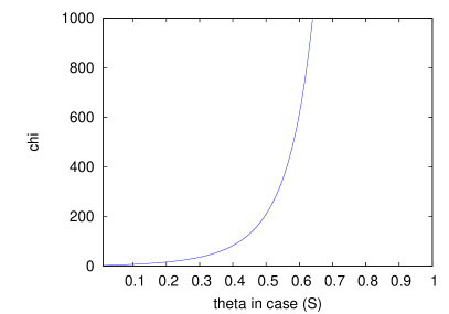
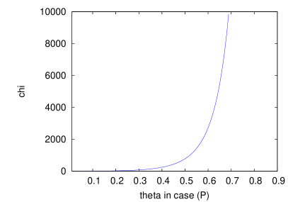
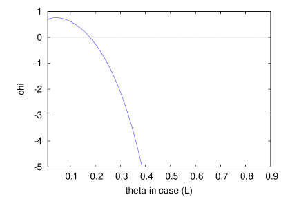
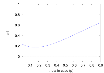
Figure 3: Plots of $\chi$ as a function of $\vartheta$. Top, left, case (S); right, case (P); bottom, left, case (L); right, case (p). Note that in all four cases, $\chi$ attains strictly positive values, showing the necessity of the requirement (2.12).

If $\bar{u}$ is chosen in this interval, the wave $\sigma_{3}$ in the construction above is not magnified by the consecutive interactions. The computations leading to the diagrams in Figure 3 are deferred to Section 5.2.

5 Technical Details

We recall here basic properties of the Euler equations (1.1), (1.4). The characteristic speeds and the right eigenvectors have the expressions

$$\begin{array}[]{l@{\quad}l@{\quad}l}\lambda_{1}=\frac{q}{\rho}-c&\lambda_{2}=\frac{q}{\rho}&\lambda_{3}=\frac{q}{\rho}+c\\[5.0pt] r_{1}=\left[\!\!\!\begin{array}[]{c}-\rho\\ \rho c-q\\ qc-E-p\end{array}\!\!\!\right]&r_{2}=\left[\!\!\!\begin{array}[]{c}\rho\\ q\\ E+p-\frac{\rho^{2}c^{2}}{\partial_{e}p}\end{array}\!\!\!\right]&r_{3}=\left[\!\!\!\begin{array}[]{c}\rho\\ q+\rho c\\ E+p+qc\end{array}\!\!\!\right]\end{array}$$ (5.1)

whose directions are chosen so that $\nabla\lambda_{i}\cdot r_{i}>0$ for $i=1,2,3$. In the case of an ideal gas, the sound speed $c=\sqrt{\partial_{\rho}p+\rho^{-2}\,p\,\partial_{e}p}$ becomes

$$c=\sqrt{\gamma(\gamma-1)e}\,.$$ (5.2)

The shock and rarefaction curves curves of the first and third family are:

$$S_{1}(u_{o},\sigma) = \left\{\begin{array}[]{l}\rho=-\sigma+\rho_{o}\\ v=v_{o}-\sqrt{-\left(p-p_{o}\right)\,\left(\frac{1}{\rho}-\frac{1}{\rho_{o}}\right)}\\ e=e_{o}-\frac{1}{2}\left(p+p_{o}\right)\,\left(\frac{1}{\rho}-\frac{1}{\rho_{o}}\right)\end{array}\right.\mbox{ for }\begin{array}[]{rcl}\sigma&\leq&0\\ \rho&\geq&\rho_{o}\\ v&\leq&v_{o}\\ S&\geq&S_{o}\end{array}$$

$$S_{3}(u_{o},\sigma) = \left\{\begin{array}[]{l}\rho=\sigma+\rho_{o}\\ v=v_{o}-\sqrt{-\left(p-p_{o}\right)\,\left(\frac{1}{\rho}-\frac{1}{\rho_{o}}\right)}\\ e=e_{o}-\frac{1}{2}\left(p+p_{o}\right)\,\left(\frac{1}{\rho}-\frac{1}{\rho_{o}}\right)\end{array}\right.\mbox{ for }\begin{array}[]{rcl}\sigma&\leq&0\\ \rho&\leq&\rho_{o}\\ v&\leq&v_{o}\\ S&\leq&S_{o}\end{array}$$

$$R_{1}(u_{o},\sigma) = \left\{\begin{array}[]{l}\rho=-\sigma+\rho_{o}\\ v=v_{o}-\displaystyle{\int_{p_{o}}^{p}[(\rho\,c)(p,S_{o})]^{-1}\,dp}\\ S(\rho,e)=S(\rho_{o},e_{o})\end{array}\right.\mbox{ for }\begin{array}[]{rcl}\sigma&\geq&0\\ \rho&\leq&\rho_{o}\\ v&\geq&v_{o}\\ e&\leq&e_{o}\end{array}$$

$$R_{3}(u_{o},\sigma) = \left\{\begin{array}[]{l}\rho=\sigma+\rho_{o}\\ v=v_{o}+\displaystyle{\int_{p_{o}}^{p}[(\rho\,c)(p,S_{o})]^{-1}\,dp}\\ S(\rho,e)=S(\rho_{o},e_{o})\end{array}\right.\mbox{ for }\begin{array}[]{rcl}\sigma&\geq&0\\ \rho&\geq&\rho_{o}\\ v&\geq&v_{o}\\ e&\geq&e_{o}\end{array}$$

The 1,2,3-Lax curves have the expressions

$$L_{1}(\sigma;\rho_{o},q_{o},E_{o}) = \left\{\begin{array}[]{lr}S_{1}(\sigma;\rho_{o},q_{o},E_{o}),&\sigma<0\\ R_{1}(\sigma;\rho_{o},q_{o},E_{o}),&\sigma\geq 0\end{array}\right.$$

$$L_{2}(\sigma;\rho_{o},q_{o},E_{o}) = \left\{\begin{array}[]{l}\rho=\sigma+\rho_{o}\\ v=v_{o}\\ p(\rho,e)=p(\rho_{o},e_{o})\end{array}\right.$$

$$L_{3}(\sigma;\rho_{o},q_{o},E_{o}) = \left\{\begin{array}[]{lr}S_{3}(\rho;\rho_{l},q_{l},E_{l}),&\sigma<0\\ R_{3}(\sigma;\rho_{o},q_{o},E_{o}),&\sigma\geq 0\end{array}\right.$$

Their reversed counterparts are

$$S_{1}^{-}(u_{o},\sigma) = \left\{\begin{array}[]{l}\rho=\sigma+\rho_{o}\\ v=v_{o}+\sqrt{-\left(p-p_{o}\right)\,\left(\frac{1}{\rho}-\frac{1}{\rho_{o}}\right)}\\ e=e_{o}-\frac{1}{2}\left(p+p_{o}\right)\,\left(\frac{1}{\rho}-\frac{1}{\rho_{o}}\right)\end{array}\right.\mbox{ for }\begin{array}[]{rcl}\sigma&\leq&0\\ \rho&\leq&\rho_{o}\\ v&\geq&v_{o}\\ S&\leq&S_{o}\end{array}$$

$$S_{3}^{-}(u_{o},\sigma) = \left\{\begin{array}[]{l}\rho=-\sigma+\rho_{o}\\ v=v_{o}+\sqrt{-\left(p-p_{o}\right)\,\left(\frac{1}{\rho}-\frac{1}{\rho_{o}}\right)}\\ e=e_{o}-\frac{1}{2}\left(p+p_{o}\right)\,\left(\frac{1}{\rho}-\frac{1}{\rho_{o}}\right)\end{array}\right.\mbox{ for }\begin{array}[]{rcl}\sigma&\leq&0\\ \rho&\geq&\rho_{o}\\ v&\geq&v_{o}\\ S&\geq&S_{o}\end{array}$$

$$R_{1}^{-}(u_{o},\sigma) = \left\{\begin{array}[]{l}\rho=\sigma+\rho_{o}\\ v=v_{o}-\displaystyle{\int_{p_{o}}^{p}[(\rho\,c)(p,S_{o})]^{-1}\,dp}\\ S(\rho,e)=S(\rho_{o},e_{o})\end{array}\right.\mbox{ for }\begin{array}[]{rcl}\sigma&\geq&0\\ \rho&\geq&\rho_{o}\\ v&\leq&v_{o}\\ e&\geq&e_{o}\end{array}$$

$$R_{3}^{-}(u_{o},\sigma) = \left\{\begin{array}[]{l}\rho=-\sigma+\rho_{o}\\ v=v_{o}+\displaystyle{\int_{p_{o}}^{p}[(\rho\,c)(p,S_{o})]^{-1}\,dp}\\ S(\rho,e)=S(\rho_{o},e_{o})\end{array}\right.\mbox{ for }\begin{array}[]{rcl}\sigma&\geq&0\\ \rho&\leq&\rho_{o}\\ v&\leq&v_{o}\\ e&\leq&e_{o}\end{array}$$

and

$$L_{1}^{-}(\sigma;\rho_{o},q_{o},E_{o}) = \left\{\begin{array}[]{lr}S_{1}^{-}(\sigma;\rho_{o},q_{o},E_{o}),&\sigma<0\\ R_{1}^{-}(\sigma;\rho_{o},q_{o},E_{o}),&\sigma\geq 0\end{array}\right.$$

$$L_{2}^{-}(\sigma;\rho_{o},q_{o},E_{o}) = \left\{\begin{array}[]{l}\rho=-\sigma+\rho_{o}\\ v=v_{o}\\ p(\rho,e)=p(\rho_{o},e_{o})\end{array}\right.$$

$$L_{3}^{-}(\sigma;\rho_{o},q_{o},E_{o}) = \left\{\begin{array}[]{ll}S_{3}^{-}(\sigma;\rho_{o},q_{o},E_{o}),&\sigma<0\\ R_{3}^{-}(\sigma;\rho_{o},q_{o},E_{o}),&\sigma\geq 0\,.\end{array}\right.$$

In the $(\rho,q,e)$ space, for a perfect ideal gas, the tangent vectors to the Lax curves are:

$$\tilde{r}_{1}=\left[\!\!\begin{array}[]{c}-1\\ -\frac{q}{\rho}-\sqrt{\gamma(\gamma-1)e}\\ -(\gamma-1)\frac{e}{\rho}\end{array}\!\!\right]\,,\ \tilde{r}_{2}=\left[\!\!\begin{array}[]{c}1\\ \frac{q}{\rho}\\ -\frac{e}{\rho}\end{array}\!\!\right]\,,\ \tilde{r}_{3}=\left[\!\!\begin{array}[]{c}1\\ \frac{q}{\rho}-\sqrt{\gamma(\gamma-1)e}\\ (\gamma-1)\frac{e}{\rho}\end{array}\!\!\right].\;$$ (5.26)

5.1 Proofs of Section 2

The following result will be of use in the proof of Proposition 2.2.

Proposition 5.1

Let $\sigma_{i}\mapsto L_{i}(u_{0},\sigma_{i})$ be the $i$-th Lax curve and $\sigma_{i}\mapsto L_{i}^{-}(u_{0},\sigma_{i})$ be the reversed $i$-th Lax curve through $u_{0}$, for $i=1,2,3$. The following equalities hold:

$$\frac{\partial L_{1}}{\partial\sigma_{1}}_{|\sigma_{1}=0}=\left(\begin{array}[]{c}1\\ \lambda_{1}(u_{o})\\ \displaystyle{\frac{E_{o}+p_{o}}{\rho_{o}}-\frac{q_{o}}{\rho_{o}}\,c_{o}}\end{array}\right),\ \frac{\partial L_{2}}{\partial\sigma_{2}}_{|\sigma_{2}=0}=\left(\begin{array}[]{c}1\\ \lambda_{2}(u_{o})\\ \displaystyle{\frac{E_{o}+p_{o}}{\rho_{o}}-\frac{\rho_{o}\,c_{o}^{2}}{\partial_{e}p_{o}}}\end{array}\right),$$

$$\frac{\partial L_{3}}{\partial\sigma_{3}}_{|\sigma_{3}=0}=\left(\begin{array}[]{c}1\\ \lambda_{3}(u_{o})\\ \displaystyle{\frac{E_{o}+p_{o}}{\rho_{o}}+\frac{q_{o}}{\rho_{o}}\,c_{o}}\end{array}\right),$$

$$\mbox{ for }i=1,2,3\qquad\frac{\partial L_{i}^{-}}{\partial\sigma_{i}}_{|\sigma_{i}=0}=-\frac{\partial L_{i}}{\partial\sigma_{i}}_{|\sigma_{i}=0},$$

$$\frac{\partial L_{i}}{\partial\rho_{o}}_{|\sigma_{i}=0}=\left(\begin{array}[]{c}1\\ 0\\ 0\end{array}\right),\quad\frac{\partial L_{i}}{\partial q_{o}}_{|\sigma_{i}=0}=\left(\begin{array}[]{c}0\\ 1\\ 0\end{array}\right),\quad\frac{\partial L_{i}}{\partial E_{o}}_{|\sigma_{i}=0}=\left(\begin{array}[]{c}0\\ 0\\ 1\end{array}\right),$$

$$+\frac{\partial L_{i}^{-}}{\partial\rho_{o}}_{|\sigma_{i}=0}=\frac{\partial L_{i}}{\partial\rho_{o}}_{|\sigma_{i}=0},\quad\frac{\partial L_{i}^{-}}{\partial q_{o}}_{|\sigma_{i}=0}=\frac{\partial L_{i}}{\partial q_{o}}_{|\sigma_{i}=0},\quad\frac{\partial L_{i}^{-}}{\partial E_{o}}_{|\sigma_{i}=0}=\frac{\partial L_{i}}{\partial E_{o}}_{|\sigma_{i}=0}.$$

The proof is immediate and, hence, omitted.

Proof of Theorem 2.2.  Following [7, Proposition 4.2], the $3\times 3$ system (1.4) defined for $x\in{\mathbb{R}}$ can be rewritten as the following $6\times 6$ system defined for $x\in{\mathbb{R}}^{+}$:

$$\left\{\begin{array}[]{l@{\qquad} rcl}\partial_{t}U+\partial_{x}\mathcal{F}(U)=0&(t,x)&\in&{\mathbb{R}}^{+}\times{\mathbb{R}}^{+}\\ b\left(U(t,0+)\right)=0&t&\in&{\mathbb{R}}^{+}\end{array}\right.$$ (5.27)

the relations between $U$ and $u=(\rho,q,E)$, between $\mathcal{F}$ and the flow in (1.4) being

$$U(t,x)=\left[\begin{array}[]{c}\rho(t,-x)\\ q(t,-x)\\ E(t,-x)\\ \rho(t,x)\\ q(t,x)\\ E(t,x)\end{array}\right]\quad\mbox{ and }\quad\mathcal{F}(U)=\left[\begin{array}[]{c}U_{2}\\ P(U_{1},U_{2},U_{3})\\ F(U_{1},U_{2},U_{3})\\ U_{5}\\ P(U_{4},U_{5},U_{6})\\ F(U_{4},U_{5},U_{6})\end{array}\right]$$

with $x\in{\mathbb{R}}^{+}$ and $E,P,F$ defined in (1.2); whereas the boundary condition in (5.27) is related to (1.5) by

$$b(U)=\Psi\left(a^{-},(U_{1},U_{2},U;_{3});a^{+},(U_{4},U_{5},U_{6})\right)$$

for fixed sections $a^{-}$ and $a^{+}$.

The thesis now follows from [6, Theorem 2.2]. Indeed, the assumptions ($\mathbf{\gamma}$), (b) and (f) therein are here satisfied. More precisely, condition ($\mathbf{\gamma}$) follows from the choice (2.6) of the subsonic region $A_{0}$. Simple computations show that condition (b) reduces to

$$\begin{array}[]{l}\det\left[D_{u^{-}}\Psi\cdot\frac{\partial L_{1}}{\partial\sigma_{1}}_{|\sigma_{1}=0}\quad D_{u^{+}}\Psi\cdot\frac{\partial L_{2}^{-}}{\partial\sigma_{2}}_{|\sigma_{2}=0}\quad D_{u^{+}}\Psi\cdot\frac{\partial L_{2}^{-}}{\partial u^{+}}_{|\sigma_{2}=0}\cdot\frac{\partial L_{3}^{-}}{\partial\sigma_{3}}_{|\sigma_{3}=0}\right]\\ =\det\left[D_{u^{-}}\Psi\cdot r_{1}(\bar{u})\quad-D_{u^{+}}\Psi\cdot r_{2}(\bar{u})\quad-D_{u^{+}}\Psi\cdot r_{3}(\bar{u})\right]\\ =\det\left[D_{u^{-}}\Psi\cdot r_{1}(\bar{u})\quad D_{u^{+}}\Psi\cdot r_{2}(\bar{u})\quad D_{u^{+}}\Psi\cdot r_{3}(\bar{u})\right],\end{array}$$

which is non zero for assumption if $\bar{u}\in A_{0}$ and $\bar{a}>0$. Condition (f) needs more care. Indeed, system (5.27) is not hyperbolic, for it is obtained gluing two copies of the Euler equations (1.4). Nevertheless, the two systems are coupled only through the boundary condition, hence the whole wave front tracking procedure in the proof of [6, Theorem 2.2] applies, see also [7, Proposition 4.5].   $\square$

Proof of Proposition 3.1.  It is immediate to check that each of the coupling conditions (3.3), (3.4), (3.5), (3.6) satisfies the requirements ($\mathbf{\Psi}$0) and ($\mathbf{\Psi}$1).

To prove that ($\mathbf{\Psi}$2) is satisfied, we use an ad hoc argument for condition (S). In all the other cases, note that the function $\Psi$ admits the representation $\Psi(a^{-},u^{-};a^{+},u^{+})=\psi(a^{-},u^{-})-\psi(a^{+},u^{+})$. Therefore, ($\mathbf{\Psi}$2) trivially holds.

We prove below (2.10) in each case separately. Note however that for any of the considered choices of $\Psi$,

$$D_{u^{+}}\Psi(a^{-},u^{-},a^{+},u^{+})_{|u=\bar{u},\,a=\bar{a}}=-D_{u^{-}}\Psi(a^{-},u^{-},a^{+},u^{+})_{|u=\bar{u},\,a=\bar{a}}$$ (5.28)

so that (2.10) reduces to

$$\det\left[D_{u^{-}}\Psi\cdot r_{1}(\bar{u})\quad D_{u^{+}}\Psi\cdot r_{2}(\bar{u})\quad D_{u^{+}}\Psi\cdot r_{3}(\bar{u})\right]$$

$$= -\det D_{u^{+}}\Psi\cdot\det\left[r_{1}(\bar{u})\quad r_{2}(\bar{u})\quad r_{3}(\bar{u})\right]\,.$$

Thus, it is sufficient to prove that $\det D_{u^{+}}\Psi(a^{-},u^{-},a^{+},u^{+})_{|u=\bar{u},\,a=\bar{a}}\neq 0$.

(S)-solutions

To prove that the coupling condition (3.3) satisfies ($\mathbf{\Psi}$2), simply use the additivity of the integral and the uniqueness of the solution to the Cauchy problem for the ordinary differential equation (3.2).

Next, we have

$$D_{u}\left(\int_{-X}^{X}p\left(\mathcal{R}^{a}(x),\mathcal{E}^{a}(x)\right)\,a^{\prime}(x)\,\mathrm{d}x\right)_{|u=\bar{u},\,a=\bar{a}}=0\,,$$

since $a^{\prime}(x)=0$ for all $x$, because $a^{-}=a^{+}=\bar{a}$. Thus, $\Psi$ in (3.3) satisfies

$$\begin{array}[]{l}D_{u^{+}}\Psi(a^{-},u^{-},a^{+},u^{+})_{|u=\bar{u},\,a=\bar{a}}\\ =\bar{a}^{3}\det\left[\!\!\begin{array}[]{ccc}0&1&0\\ -\frac{\bar{q}^{2}}{\bar{\rho}^{2}}+{\partial_{\rho}\bar{p}}+\frac{{\partial_{e}\bar{p}}}{\bar{\rho}}\left(\frac{\bar{q}^{2}}{\bar{\rho}^{2}}-\frac{\bar{E}}{\bar{\rho}}\right)&\frac{\bar{q}}{\bar{\rho}}\left(2-\frac{{\partial_{e}\bar{p}}}{\bar{\rho}}\right)&\frac{{\partial_{e}\bar{p}}}{\bar{\rho}}\\ -\frac{\bar{q}}{\bar{\rho}}\left({\partial_{\rho}\bar{p}}+\frac{{\partial_{e}\bar{p}}}{\bar{\rho}}\left(\frac{\bar{q}^{2}}{\bar{\rho}^{2}}-\frac{\bar{E}}{\bar{\rho}}\right)-\frac{\bar{E}+\bar{p}}{\bar{\rho}}\right)&\frac{\bar{E}+\bar{p}}{\bar{\rho}}-\frac{{\partial_{e}\bar{p}}}{\bar{\rho}}\frac{\bar{q}^{2}}{\bar{\rho}^{2}}&-\frac{\bar{q}}{\bar{\rho}}\left(\frac{{\partial_{e}\bar{p}}}{\bar{\rho}}+1\right)\end{array}\!\!\right]\!\!\\ =-\bar{a}^{3}\,\lambda_{1}(\bar{u})\,\lambda_{2}(\bar{u})\,\lambda_{3}(\bar{u}),\end{array}$$

which is non zero if $\bar{u}\in A_{0}$.

(P)-solutions

Concerning condition (3.4), we have

$$\begin{array}[]{l}D_{u^{+}}\Psi(a^{-},u^{-},a^{+},u^{+})_{|u=\bar{u},\,a=\bar{a}}\\ =\det\left[\!\!\begin{array}[]{ccc}0&\bar{a}&0\\ -\frac{\bar{q}^{2}}{\bar{\rho}^{2}}+{\partial_{\rho}\bar{p}}+\frac{{\partial_{e}\bar{p}}}{\bar{\rho}}\left(\frac{\bar{q}^{2}}{\bar{\rho}^{2}}-\frac{\bar{E}}{\bar{\rho}}\right)&\frac{\bar{q}}{\bar{\rho}}\left(2-\frac{{\partial_{e}\bar{p}}}{\bar{\rho}}\right)&\frac{{\partial_{e}\bar{p}}}{\bar{\rho}}\\ -\bar{a}\frac{\bar{q}}{\bar{\rho}}\left({\partial_{\rho}\bar{p}}+\frac{{\partial_{e}\bar{p}}}{\bar{\rho}}\left(\frac{\bar{q}^{2}}{\bar{\rho}^{2}}-\frac{\bar{E}}{\bar{\rho}}\right)-\frac{\bar{E}+\bar{p}}{\bar{\rho}}\right)&\bar{a}\frac{\bar{E}+\bar{p}}{\bar{\rho}}-\bar{a}\frac{{\partial_{e}\bar{p}}}{\bar{\rho}}\frac{\bar{q}^{2}}{\bar{\rho}^{2}}&-\bar{a}\frac{\bar{q}}{\bar{\rho}}\left(\frac{{\partial_{e}\bar{p}}}{\bar{\rho}}+1\right)\end{array}\!\!\right]\!\!\\ =-\bar{a}^{2}\lambda_{1}(\bar{u})\lambda_{2}(\bar{u})\lambda_{3}(\bar{u}),\end{array}$$

which is non zero if $\bar{u}\in A_{0}$.

(L)-solution

For condition (3.5) the computations very similar to the above case:

$$D_{u^{+}}\Psi(a^{-},u^{-},a^{+},u^{+})_{|u=\bar{u},\,a=\bar{a}}=-\bar{a}^{3}\lambda_{1}(\bar{u})\lambda_{2}(\bar{u})\lambda_{3}(\bar{u}),$$

which is non zero if $\bar{u}\in A_{0}$.

(p)-solution

Finally, concerning condition (3.6),

$$\begin{array}[]{l}D_{u^{+}}\Psi(a^{-},u^{-},a^{+},u^{+})_{|u=\bar{u},\,a=\bar{a}}\\ =\det\left[\!\!\begin{array}[]{ccc}0&\bar{a}&0\\ {\partial_{\rho}\bar{p}}+\frac{{\partial_{e}\bar{p}}}{\bar{\rho}}\left(\frac{\bar{q}^{2}}{\bar{\rho}^{2}}-\frac{\bar{E}}{\bar{\rho}}\right)&-\frac{\bar{q}}{\bar{\rho}^{2}}{\partial_{e}\bar{p}}&\frac{{\partial_{e}\bar{p}}}{\bar{\rho}}\\ -\bar{a}\frac{\bar{q}}{\bar{\rho}}\left({\partial_{\rho}\bar{p}}+\frac{{\partial_{e}\bar{p}}}{\bar{\rho}}\left(\frac{\bar{q}^{2}}{\bar{\rho}^{2}}-\frac{\bar{E}}{\bar{\rho}}\right)-\frac{\bar{E}+\bar{p}}{\bar{\rho}}\right)&\bar{a}\frac{\bar{E}+\bar{p}}{\bar{\rho}}-\bar{a}\frac{{\partial_{e}\bar{p}}}{\bar{\rho}}\frac{\bar{q}^{2}}{\bar{\rho}^{2}}&-\bar{a}\frac{\bar{q}}{\bar{\rho}}\left(\frac{{\partial_{e}\bar{p}}}{\bar{\rho}}+1\right)\end{array}\!\!\right]\!\!\\ =\bar{a}^{2}\lambda_{2}(\bar{u})\left(c^{2}+\lambda_{2}^{2}(\bar{u})\frac{{\partial_{e}\bar{p}}}{\bar{\rho}}\right),\end{array}$$

which is non zero if $\bar{u}\in A_{0}$ and if the fluid is perfect, i.e. (1.3) holds.   $\square$

5.2 Computation of $\chi$ in (4.5)

The Case of Condition (S)

Let $\Psi$ be defined in (3.3) and set

$$\Sigma(a^{-},a^{+},u)=\int_{-X}^{X}p\left(\mathcal{R}^{a}(x),\mathcal{E}^{a}(x)\right)\,a^{\prime}(x)dx$$

where the functions $\mathcal{R}^{a},\mathcal{E}^{a}$ have the same meaning as in (3.3). A perturbative method allows to compute the solution to (3.2) with a second order accuracy in $(\Delta a)/a$. Then, long elementary computations allow to get explicitly the terms $H$ and $G$ in (4.2) of the second order expansion of $T$:

$$H(\rho,q,e) = \left[\begin{array}[]{l}\displaystyle-{{\,\vartheta^{3}-4\,\vartheta^{2}+5\,\vartheta-2}\over{\,\vartheta^{3}-3\,\vartheta^{2}+3\,\vartheta-1}}\;\rho\\ \displaystyle-q\\ \displaystyle-{{2\left(-\vartheta^{3}+2\,\vartheta^{2}-\vartheta\right)}\over{3\left(\vartheta^{3}-3\,\vartheta^{2}+3\,\vartheta-1\right)}}\;e\end{array}\right]$$

$$G(\rho,q,e) = \left[\begin{array}[]{l}\displaystyle-{{4\left(\vartheta^{3}-2\,\vartheta^{2}\right)}\over{3\left(\vartheta^{3}-3\,\vartheta^{2}+3\,\vartheta-1\right)}}\;\rho\\ q\\ \displaystyle-{{70\,\vartheta^{4}-257\,\vartheta^{3}+342\,\vartheta^{2}-207\,\vartheta+36}\over{18\left(\vartheta^{3}-3\,\vartheta^{2}+3\,\vartheta-1\right)}}\;e\end{array}\right]\,.$$

Moreover, the coefficients $f_{1}$, $f_{2}$ in (4.3) read

$$f_{1}(\vartheta) = -{{-3\,\vartheta+\left(\vartheta-3\right)\,\sqrt{\vartheta}-3}\over{6\,\sqrt{\vartheta}\,\left(\vartheta-1\right)-6\left(\vartheta-1\right)}}$$

$$f_{2}(\vartheta) = {{\sqrt{\vartheta}\,\left(126\,\vartheta^{4}-505\,\vartheta^{3}+758\,\vartheta^{2}-489\,\vartheta+270\right)\over{72\left(\sqrt{\vartheta}\,\left(\vartheta^{3}-3\,\vartheta^{2}+3\,\vartheta-1\right)-\vartheta^{3}+3\,\vartheta^{2}-3\,\vartheta+1\right)}}}$$

$$+{{42\,\vartheta^{4}-183\,\vartheta^{3}+278\,\vartheta^{2}+33\,\vartheta+54}\over{72\left(\sqrt{\vartheta}\,\left(\vartheta^{3}-3\,\vartheta^{2}+3\,\vartheta-1\right)-\vartheta^{3}+3\,\vartheta^{2}-3\,\vartheta+1\right)}}\,.$$

Next, $\chi$ is given by

$$\chi={{\sqrt{\vartheta}\,\left(126\,\vartheta^{4}-506\,\vartheta^{3}+773\,\vartheta^{2}-480\,\vartheta+279\right)+42\,\vartheta^{4}-174\,\vartheta^{3}+311\,\vartheta^{2}+96\,\vartheta+45}\over{36\left(\sqrt{\vartheta}\,\left(\vartheta^{3}-3\,\vartheta^{2}+3\,\vartheta-1\right)-\vartheta^{3}+3\,\vartheta^{2}-3\,\vartheta+1\right)}}\,.$$

The Case of Condition (P)

Let $\Psi$ be defined in (3.4). With reference to (4.2), we show below explicitly the terms $H$ and $G$ in (4.2) of the second order expansion of $T$,

$$H(\rho,q,e) = \left[\begin{array}[]{l}\displaystyle{{8\left(-\vartheta^{3}+2\,\vartheta^{2}-\vartheta\right)}\over{3\left(\vartheta^{3}-3\,\vartheta^{2}+3\,\vartheta-1\right)}}\;\rho\\ \displaystyle-q\\ \displaystyle-{{2\left(5\,\vartheta^{4}-7\,\vartheta^{3}-\vartheta^{2}+3\,\vartheta\right)}\over{9\left(\vartheta^{3}-3\,\vartheta^{2}+3\,\vartheta-1\right)}}\;e\end{array}\right]$$

$$G(\rho,q,e) = \left[\begin{array}[]{l}\displaystyle{{64\left(\vartheta^{3}+3\,\vartheta^{2}\right)}\over{27\left(\vartheta^{3}-3\,\vartheta^{2}+3\,\vartheta-1\right)}}\;\rho\\ q\\ \displaystyle-{{565\,\vartheta^{4}-1599\,\vartheta^{3}+927\,\vartheta^{2}-405\,\vartheta}\over{81\left(\vartheta^{3}-3\,\vartheta^{2}+3\,\vartheta-1\right)}}\;e\end{array}\right]\,.$$

Moreover, the coefficients $f_{1}$, $f_{2}$ in (4.3) read

$$f_{1}(\vartheta) = {{\sqrt{\vartheta}\,\left(9\,\vartheta^{2}+2\,\vartheta-27\right)+3\,\vartheta^{2}-42\,\vartheta-9}\over{18\sqrt{\vartheta}\,\left(\vartheta-1\right)-18\left(\vartheta-1\right)}}$$

$$f_{2}(\vartheta) = {{\sqrt{\vartheta}\,\left(154\,\vartheta^{5}+931\,\vartheta^{4}-4416\,\vartheta^{3}+6570\,\vartheta^{2}+990\,\vartheta+891\right)}\over{324\left(\sqrt{\vartheta}\,\left(\vartheta^{3}-3\,\vartheta^{2}+3\,\vartheta-1\right)-\vartheta^{3}+3\,\vartheta^{2}-3\,\vartheta+1\right)}}$$

$$+{{86\,\vartheta^{5}-311\,\vartheta^{4}-752\,\vartheta^{3}+7038\,\vartheta^{2}+1026\,\vartheta+81}\over{324\left(\sqrt{\vartheta}\,\left(\vartheta^{3}-3\,\vartheta^{2}+3\,\vartheta-1\right)-\vartheta^{3}+3\,\vartheta^{2}-3\,\vartheta+1\right)}}.$$

Next, $\chi$ is given by

$$\chi = {{\sqrt{\vartheta}\,\left(407\,\vartheta^{5}+1931\,\vartheta^{4}-7858\,\vartheta^{3}+14766\,\vartheta^{2}+1179\,\vartheta+1863\right)}\over{324\left(\sqrt{\vartheta}\,\left(\vartheta^{3}-3\,\vartheta^{2}+3\,\vartheta-1\right)-\vartheta^{3}+3\,\vartheta^{2}-3\,\vartheta+1\right)}}$$

$$+{{-23\,\vartheta^{5}+141\,\vartheta^{4}+2002\,\vartheta^{3}+15714\,\vartheta^{2}+2565\,\vartheta+81}\over{324\left(\sqrt{\vartheta}\,\left(\vartheta^{3}-3\,\vartheta^{2}+3\,\vartheta-1\right)-\vartheta^{3}+3\,\vartheta^{2}-3\,\vartheta+1\right)}}\,.$$

The Case of Condition (L)

Let $\Psi$ be defined in (3.5). Then,

$$H(\rho,q,e)=\left[\begin{array}[]{l}-\rho\\ -q\\ 0\end{array}\right]\qquad\mbox{ and }\qquad G(\rho,q,e)=\left[\begin{array}[]{l}\displaystyle-{{4\,\vartheta}\over{3\left(\vartheta-1\right)}}\;\rho\\ q\\ \displaystyle-{{35\,\vartheta^{2}-9\left(4\,\vartheta-1\right)}\over{9\left(\vartheta-1\right)}}\;e\end{array}\right].$$

The coefficients $f_{1}$, $f_{2}$ in (4.3) read

$$f_{1}(\vartheta) = 0$$

$$f_{2}(\vartheta) = {{\sqrt{\vartheta}\,\left(63\,\vartheta^{2}-106\,\vartheta+27\right)+21\,\vartheta^{2}-78\,\vartheta+9}\over{36\left(\sqrt{\vartheta}\,\left(\vartheta-1\right)-\vartheta+1\right)}},$$

so that $\chi$ is

$$\chi={{\sqrt{\vartheta}\,\left(63\,\vartheta^{2}-106\,\vartheta+27\right)+21\,\vartheta^{2}-78\,\vartheta+9}\over{18\left(\sqrt{\vartheta}\,\left(\vartheta-1\right)-\vartheta+1\right)}}\,.$$

The Case of Condition (p)

Let $\Psi$ be defined in (3.6). With reference to (4.2),

$$H(\rho,q,e) = \left[\begin{array}[]{l}\displaystyle-{{2\left(4\,\vartheta^{3}+12\,\vartheta^{2}+9\,\vartheta\right)}\over{4\left(2\,\vartheta^{3}+9\,\vartheta^{2}\right)+27\left(2\,\vartheta+1\right)}}\;\rho\\ -q\\ \displaystyle{{2\left(4\,\vartheta^{3}+12\,\vartheta^{2}+9\,\vartheta\right)}\over{4\left(2\,\vartheta^{3}+9\,\vartheta^{2}\right)+27\left(2\,\vartheta+1\right)}}\;e\end{array}\right]$$

$$G(\rho,q,e) = \left[\begin{array}[]{l}\displaystyle-{{4\left(\vartheta^{3}+3\,\vartheta^{2}\right)}\over{4\left(2\,\vartheta^{3}+9\,\vartheta^{2}\right)+27\left(2\,\vartheta+1\right)}}\;\rho\\ q\\ \displaystyle{{12\left(\vartheta^{3}+2\,\vartheta^{2}\right)}\over{4\left(2\,\vartheta^{3}+9\,\vartheta^{2}\right)+27\left(2\,\vartheta+1\right)}}\;e\end{array}\right],$$

with $f_{1}$ and $f_{2}$ given by

$$f_{1}(\vartheta) = {{-2\,\vartheta^{2}+4\,\vartheta^{{{3}\over{2}}}+3\,\vartheta-9}\over{2\left(4\,\vartheta^{2}+12\,\vartheta+9\right)}}$$

$$f_{2}(\vartheta) = {{32\,\vartheta^{4}+8\,\sqrt{\vartheta}\,\left(4\,\vartheta^{3}+9\,\vartheta^{2}-9\,\vartheta\right)+316\,\vartheta^{3}+558\,\vartheta^{2}+216\,\vartheta+81}\over{6\left(16\,\vartheta^{4}+96\,\vartheta^{3}+216\,\vartheta^{2}+216\,\vartheta+81\right)}}\,,$$

so that

$$\chi={{60\,\vartheta^{4}+96\,\sqrt{\vartheta}\,\left(\vartheta^{3}+\vartheta^{2}-3\,\vartheta\right)+700\,\vartheta^{3}+1107\,\vartheta^{2}-54\,\vartheta+81}\over{6\left(16\,\vartheta^{4}+96\,\vartheta^{3}+216\,\vartheta^{2}+216\,\vartheta+81\right)}}.$$

$$\vartheta^{+} = \vartheta-{{\sqrt{\vartheta}\,\left(\left(\sigma_{3}^{-}+6\right)\,\vartheta^{2}+18\,\vartheta-9\,\sigma_{3}^{-}\right)+2\left(3-2\,\sigma_{3}^{-}\right)\,\vartheta^{2}+6\left(2\,\sigma_{3}^{-}+3\right)\,\vartheta}\over{9\sqrt{\vartheta}\,\left(\vartheta-1\right)+9\left(\vartheta-1\right)}}\frac{\Delta a}{a}$$

$$- {{\sqrt{\vartheta}\,\left(14\left(11\,\sigma_{3}^{-}-30\right)\,\vartheta^{5}+\left(990-301\,\sigma_{3}^{-}\right)\,\vartheta^{4}+3\left(25\,\sigma_{3}^{-}-236\right)\,\vartheta^{3}+\left(111\,\sigma_{3}^{-}-18\right)\,\vartheta^{2}+45\left(12-\,\sigma_{3}^{-}\right)\,\vartheta-378\,\sigma_{3}^{-}\right)}\over{108\left(\sqrt{\vartheta}\,\left(\vartheta^{3}-3\,\vartheta^{2}+3\,\vartheta-1\right)+\vartheta^{3}-3\,\vartheta^{2}+3\,\vartheta-1\right)}}\left(\frac{\Delta a}{a}\right)^{2}$$

$$-{{4\left(217\,\sigma_{3}^{-}-105\right)\,\vartheta^{5}+2\left(495-1489\,\sigma_{3}^{-}\right)\,\vartheta^{4}+4\left(928\,\sigma_{3}^{-}-177\right)\,\vartheta^{3}-2\left(1077\,\sigma_{3}^{-}-9\right)\,\vartheta^{2}+24\left(26\,\sigma_{3}^{-}+15\right)\,\vartheta}\over{108\left(\sqrt{\vartheta}\,\left(\vartheta^{3}-3\,\vartheta^{2}+3\,\vartheta-1\right)+\vartheta^{3}-3\,\vartheta^{2}+3\,\vartheta-1\right)}}\left(\frac{\Delta a}{a}\right)^{2}$$

$$\vartheta^{+} = \vartheta-{{\sqrt{\vartheta}\,\left(\left(11\,\sigma_{3}^{-}-30\right)\,\vartheta^{3}+\left(-19\,\sigma_{3}^{-}-108\right)\,\vartheta^{2}+9\left(5\,\sigma_{3}^{-}-6\right)\,\vartheta+27\,\sigma_{3}^{-}\right)+2\left(31\,\sigma_{3}^{-}-15\right)\,\vartheta^{3}-36\left(\sigma_{3}^{-}+3\right)\,\vartheta^{2}-18\left(5\,\sigma_{3}^{-}+3\right)\,\vartheta}\over{27\sqrt{\vartheta}\,\left(\vartheta-1\right)+27\left(\vartheta-1\right)}}\frac{\Delta a}{a}$$

$$- {{\sqrt{\vartheta}\,\left(2\left(233\,\sigma_{3}^{-}-300\right)\,\vartheta^{6}+\left(1279\,\sigma_{3}^{-}-5310\right)\,\vartheta^{5}+\left(5400-2543\,\sigma_{3}^{-}\right)\,\vartheta^{4}+6\left(677\,\sigma_{3}^{-}+1242\right)\,\vartheta^{3}+36\left(109-297\,\sigma_{3}^{-}\right)\,\vartheta^{2}+729\left(2-5\,\sigma_{3}^{-}\right)\,\vartheta-1215\,\sigma_{3}^{-}\right)}\over{486\left(\sqrt{\vartheta}\,\left(\vartheta^{3}-3\,\vartheta^{2}+3\,\vartheta-1\right)+\vartheta^{3}-3\,\vartheta^{2}+3\,\vartheta-1\right)}}\left(\frac{\Delta a}{a}\right)^{2}$$

$$-{{4\left(601\,\sigma_{3}^{-}-150\right)\,\vartheta^{6}+2\left(3521\,\sigma_{3}^{-}-2655\right)\,\vartheta^{5}+8\left(225-3814\,\sigma_{3}^{-}\right)\,\vartheta^{4}+36\left(655\,\sigma_{3}^{-}+207\right)\,\vartheta^{3}+108\left(53\,\sigma_{3}^{-}+36\right)\,\vartheta^{2}+162\left(9\,\sigma_{3}^{-}+25\right)\,\vartheta}\over{486\left(\sqrt{\vartheta}\,\left(\vartheta^{3}-3\,\vartheta^{2}+3\,\vartheta-1\right)+\vartheta^{3}-3\,\vartheta^{2}+3\,\vartheta-1\right)}}\left(\frac{\Delta a}{a}\right)^{2}$$

$$\vartheta^{+} = \vartheta-{{\sqrt{\vartheta}\,\left(\left(77\,\sigma_{3}^{-}-210\right)\,\vartheta^{3}+\left(-13\,\sigma_{3}^{-}-36\right)\,\vartheta^{2}+27\left(\sigma_{3}^{-}+2\right)\,\vartheta-27\,\sigma_{3}^{-}\right)2+\left(217\,\sigma_{3}^{-}-105\right)\,\vartheta^{3}-4\left(147\,\sigma_{3}^{-}+9\right)\,\vartheta^{2}+18\left(5\,\sigma_{3}^{-}+3\right)\,\vartheta}\over{54\sqrt{\vartheta}\,\left(\vartheta-1\right)+54\left(\vartheta-1\right)}}\left(\frac{\Delta a}{a}\right)^{2}$$

$$\vartheta^{+} = \vartheta+{{-2\left({\sigma_{3}^{-}}+6\right)\,\vartheta^{3}+\sqrt{\vartheta}\,\left(10\,{\sigma_{3}^{-}}\,\vartheta^{2}+27\,{\sigma_{3}^{-}}\,\vartheta+27\,{\sigma_{3}^{-}}\right)+3\left({\sigma_{3}^{-}}-18\right)\,\vartheta^{2}-9\left({\sigma_{3}^{-}}+6\right)\,\vartheta}\over{3\left(4\,\vartheta^{2}+12\,\vartheta+9\right)}}\frac{\Delta a}{a}$$

$$- {{-48\left({\sigma_{3}^{-}}+5\right)\,\vartheta^{5}+\sqrt{\vartheta}\,\left(144\,{\sigma_{3}^{-}}\,\vartheta^{4}+780\,{\sigma_{3}^{-}}\,\vartheta^{3}+2214\,{\sigma_{3}^{-}}\,\vartheta^{2}+1944\,{\sigma_{3}^{-}}\,\vartheta+1215\,{\sigma_{3}^{-}}\right)}\over{48\left(2\,\vartheta^{4}+12\,\vartheta^{3}+27\,\vartheta^{2}+27\,\vartheta+12\right)}}\left(\frac{\Delta a}{a}\right)^{2}$$

$$- {{-4\left(91\,{\sigma_{3}^{-}}+342\right)\,\vartheta^{4}-54\left(11\,{\sigma_{3}^{-}}+56\right)\,\vartheta^{3}-216\left(2\,{\sigma_{3}^{-}}+15\right)\,\vartheta^{2}-81\left(5\,{\sigma_{3}^{-}}+18\right)\,\vartheta}\over{48\left(2\,\vartheta^{4}+12\,\vartheta^{3}+27\,\vartheta^{2}+27\,\vartheta+12\right)}}\left(\frac{\Delta a}{a}\right)^{2}$$

Above are the values of $\vartheta^{+}$ in the cases (S), (P), (L) and (p).

References

[1]
M. K. Banda, M. Herty, and A. Klar.
Coupling conditions for gas networks governed by the isothermal
Euler equations.
Netw. Heterog. Media, 1(2):295–314 (electronic), 2006.
[2]
M. K. Banda, M. Herty, and A. Klar.
Gas flow in pipeline networks.
Netw. Heterog. Media, 1(1):41–56 (electronic), 2006.
[3]
A. Bressan.
Hyperbolic systems of conservation laws, volume 20 of Oxford Lecture Series in Mathematics and its Applications.
Oxford University Press, Oxford, 2000.
The one-dimensional Cauchy problem.
[4]
R. M. Colombo and M. Garavello.
On the -system at a junction.
In Control methods in PDE-dynamical systems, volume 426 of Contemp. Math., pages 193–217. Amer. Math. Soc., Providence, RI, 2007.
[5]
R. M. Colombo and M. Garavello.
On the 1D modeling of fluid flowing through a junction.
Preprint, 2009.
[6]
R. M. Colombo and G. Guerra.
On general balance laws with boundary.
Preprint, http://arxiv.org/abs/0810.5246, 2008.
[7]
R. M. Colombo, G. Guerra, M. Herty, and V. Sachers.
Modeling and optimal control of networks of pipes and canals.
SIAM J. Math. Anal., 48(3):2032–2050, 2009.
[8]
R. M. Colombo, M. Herty, and V. Sachers.
On conservation laws at a junction.
SIAM J. Math. Anal., 40(2):605–622, 2008.
[9]
R. M. Colombo and F. Marcellini.
Smooth and discontinuous junctions in the p-system.
J. Math. Anal. Appl., pages 440–456, 2010.
[10]
R. M. Colombo and C. Mauri.
Euler system at a junction.
Journal of Hyperbolic Differential Equations, 5(3):547–568,
2007.
[11]
M. Garavello and B. Piccoli.
Traffic flow on networks, volume 1 of AIMS Series on
Applied Mathematics.
American Institute of Mathematical Sciences (AIMS), Springfield, MO,
2006.
Conservation laws models.
[12]
P. Goatin and P. G. LeFloch.
The Riemann problem for a class of resonant hyperbolic systems of
balance laws.
Ann. Inst. H. Poincaré Anal. Non Linéaire, 21(6):881–902,
2004.
[13]
G. Guerra, F. Marcellini, and V. Schleper.
Balance laws with integrable unbounded source.
SIAM J. Math. Anal., 41(3), 2009.
[14]
H. Holden and N. H. Risebro.
Riemann problems with a kink.
SIAM J. Math. Anal., 30(3):497–515 (electronic), 1999.
[15]
T. P. Liu.
Nonlinear stability and instability of transonic flows through a
nozzle.
Comm. Math. Phys., 83(2):243–260, 1982.
[16]
J. Smoller.
Shock waves and reaction-diffusion equations.
Springer-Verlag, New York, second edition, 1994.
[17]
G. B. Whitham.
Linear and nonlinear waves.
John Wiley & Sons Inc., New York, 1999.
Reprint of the 1974 original, A Wiley-Interscience Publication.