Quantum bright soliton in a disorder potential

Abstract

At very low temperature, a quasi-one-dimensional ensemble of atoms with attractive interactions tend to form a bright soliton. When exposed to a sufficiently weak external potential, the shape of the soliton is not modified, but its external motion is affected. We develop in detail the Bogoliubov approach for the problem, treating, in a non-perturbative way, the motion of the center of mass of the soliton. Quantization of this motion allows us to discuss its long time properties. In particular, in the presence of a disordered potential, the quantum motion of the center of mass of a bright soliton may exhibit Anderson localization, on a localization length which may be much larger than the soliton size and could be observed experimentally.

I Introduction

Anderson localization is a localization effect predicted to take place for a wave propagating in a disordered potential anderson1958 . It is due to multiply scattered waves from random defects and yields exponentially localized density profiles, resulting in a complete suppression of the usual diffusive transport associated with incoherent wave scattering lee1985 . While in the three dimensional world, one may observe a transition between extended and localized states, in a one-dimensional (1D) world, Anderson localization is a typical feature of the motion in a disordered potential vantiggelen1999 .

Cold atoms form a wonderful toolbox for controlling parameters of the system under study jaksch . It comes out as no surprise that attempts have been made for a direct observation of the Anderson localization in cold atoms settings. Already the first attempts bodzio ; inguscio ; fort ; aspect ; wir ; wir2 have revealed that the presence of atomic interactions may deeply affect the physics of the problem and make the observation of the localization non trivial. Further theoretical studies LSP2007 ; Lugan2007 ; skipetrov2008 were followed by successful observations of the phenomenon made possible by going to the regime of very weakly interacting particles Billy2008 . While in that work a random speckle potential was used, in another attempt ingu2008 a quasi-periodic version of the potential using superposition of laser beams was created resulting in the observation of Aubry-André AA localization for noninteracting atoms.

Anderson localization is a one-body phenomenon, and it is important to understand how it is modified when interactions between particles – in our case, cold atoms – are taken into account. In the absence of any external potential, at zero temperature, 1D particles interacting attractively tend to cluster together, forming a bright soliton. Explicit solutions of the many-body problem can be found for a contact interaction McGuire64 . Altogether, a bright soliton appears as a composite particle, whose position is given by the center of mass of the constituting atoms and a mass equal to the sum of the mass of the atoms (see next section). Using external potentials, it has been experimentally shown how to put solitons in motion brightexp . The purpose of this contribution is to discuss what happens to a bright soliton exposed to a weak and smooth disordered potential kivshar ; others . Of course, if that potential was sufficiently strong, it could probably destroy the soliton altogether, break it into pieces etc. We are, however, interested in the other limit when the external potential is sufficiently weak and smooth not to perturb the soliton shape. It is then quite reasonable to expect that, if this weak potential is of random nature (disorder) that the soliton as a composite particle, undergoes multiple scattering, diffusive motion and eventually Anderson localization. In a recent short contribution ours we have shown that this is indeed the case by considering the effective quantum motion of the soliton. The present work brings a detailed derivation of the effective Hamiltonian applied before, and shows examples of the corresponding localized eigenstates. It provides thus a complementary material to our previous work ours .

II Mean field description

II.1 Equations of motion for a bright soliton in a disorder potential

Consider an ensemble of cold atoms (bosons) with attractive interactions at zero temperature. We assume a strong harmonic transverse confinement so a one-dimensional approximation can be used. In the mean field approach, a $c$-number function $\phi$ takes the place of the bosonic field operator $\hat{\psi}$. $\phi$ is a solution of the Gross-Pitaevskii equation

$$i\partial_{t}\phi=-\frac{1}{2}\partial_{z}^{2}\phi-|\phi|^{2}\phi,$$ (1)

where we have adopted the following natural units for energy, length and time, respectively

$$E_{0} = 4m\omega_{\perp}^{2}a^{2},$$ (2)

$$l_{0} = \frac{\hbar}{2|a|m\omega_{\perp}},$$ (3)

$$t_{0} = \frac{\hbar}{4a^{2}m\omega_{\perp}^{2}}.$$ (4)

The transverse harmonic confinement frequency is denoted by $\omega_{\perp}$, $a$ is the atomic $s$-wave scattering length, and $m$ the mass of an atom. We normalize $\phi$ to the total number of particles $N$. Eq.(1) admits a stationary bright soliton solution $e^{-i\mu t}\phi_{0}$ zakharov , where

$$\phi_{0}(z-q)=\sqrt{\frac{N}{2\xi}}\frac{e^{-i\theta}}{\cosh[(z-q)/\xi]},$$ (5)

the chemical potential $\mu=-N^{2}/8$ and the soliton width $\xi=2/N$. This bright solitonic solution minimizes the energy functional

$$E=\int dz\left[\frac{1}{2}|\partial_{z}\phi|^{2}-\frac{1}{2}|\phi|^{4}-\mu|\phi|^{2}\right].$$ (6)

Observe that eq. (5) allows for an arbitrary center-of-mass (CM) position $q$ and an arbitrary global phase $\theta$.

Suppose the soliton is placed in a weak and smooth disorder potential, $V(z)$, with variance $V_{0}^{2}$ and correlation length $\sigma_{0}$. We will concentrate on the case when $\sigma_{0}<\xi$ but the approach we present is general. Linearization of the Gross-Pitaevskii equation allows us to describe the perturbation of the soliton due to the presence of a weak potential castin . Indeed, the substitution

$$e^{-i\mu t}[\phi_{0}+\delta\phi],$$ (7)

into (1) supplemented with the potential $V(z)$ leads to the following inhomogeneous time-dependent Bogoliubov equations

$$i\partial_{t}\left(\begin{array}[]{c}\delta\phi\\ \delta\phi^{*}\end{array}\right)={\cal L}\left(\begin{array}[]{c}\delta\phi\\ \delta\phi^{*}\end{array}\right)+\left(\begin{array}[]{c}S\\ -S^{*}\end{array}\right),$$ (8)

where

$${\cal L}=\left(\begin{array}[]{cc}-\frac{1}{2}\partial^{2}_{z}-2|\phi_{0}|^{2}-\mu&-\phi_{0}^{2}\\ \phi_{0}^{*2}&\frac{1}{2}\partial^{2}_{z}+2|\phi_{0}|^{2}+\mu\end{array}\right),$$ (11)

and

$$S=V(z)\;\phi_{0}(z-q).$$ (12)

In Eq. (8) we have neglected terms of order higher than ${\cal O}(\delta\phi,V)$. Solution of (8) can be expanded in right eigenvectors and corresponding adjoint modes of the non-hermitian operator ${\cal L}$. However, this operator is not diagonalizable castin ; lewenstein ; dziarmaga04 . For all eigenvectors $(u_{n},v_{n})$ corresponding to non-zero eigenvalues $E_{n}$, the adjoint modes are left eigenvectors of the $\cal L$. That is no longer true for the zero-eigenvalue modes. There are two zero modes in our system

$$\left(\begin{array}[]{c}u_{\theta}\\ v_{\theta}\end{array}\right)=i\partial_{\theta}\left(\begin{array}[]{c}\phi_{0}\\ \phi_{0}^{*}\end{array}\right),\quad\left(\begin{array}[]{c}u_{q}\\ v_{q}\end{array}\right)=i\partial_{q}\left(\begin{array}[]{c}\phi_{0}\\ \phi_{0}^{*}\end{array}\right),$$ (13)

which are related to a small modification of the global phase of the solution (5) and to a small shift of the CM, respectively dziarmaga04 ; ours . As both modifications cost no energy they appear as zero modes of the ${\cal L}$ operator. Indeed, it is consistent with quadratic expansion of the energy functional,

$$E={\rm const}+\frac{1}{2}\int dz\;(\delta\phi^{*},-\delta\phi)\;{\cal L}\;\left(\begin{array}[]{c}\delta\phi\\ \delta\phi^{*}\end{array}\right),$$ (14)

where we see that contributions to soliton perturbation from zero modes do not change $E$. The modes adjoint to the zero modes are

$$\left(\begin{array}[]{c}u_{\theta}^{\rm ad}\\ v_{\theta}^{\rm ad}\end{array}\right)=\partial_{N}\left(\begin{array}[]{c}\phi_{0}\\ \phi_{0}^{*}\end{array}\right),\quad\left(\begin{array}[]{c}u_{q}^{\rm ad}\\ v_{q}^{\rm ad}\end{array}\right)=i\frac{z-q}{N}\left(\begin{array}[]{c}\phi_{0}\\ -\phi_{0}^{*}\end{array}\right),$$ (15)

which has been found by solving

$${\cal L}\left(\begin{array}[]{c}u_{\theta,q}^{\text{ad}}\\ v_{\theta,q}^{\text{ad}}\end{array}\right)=\frac{1}{M_{\theta,q}}\left(\begin{array}[]{c}u_{\theta,q}\\ v_{\theta,q}\end{array}\right),$$ (16)

where $M_{\theta}$ and $M_{q}$ are determined by the requirements $\langle u_{\theta}^{\text{ad}}|u_{\theta}\rangle-\langle v_{\theta}^{\text{ad}}|v_{\theta}\rangle=1$ and $\langle u_{q}^{\text{ad}}|u_{q}\rangle-\langle v_{q}^{\text{ad}}|v_{q}\rangle=1$ castin ; lewenstein ; dziarmaga04 ; ours . It turns out that

$$M_{\theta}=-\frac{4}{N},\quad M_{q}=N.$$ (17)

The latter is equal to the total mass of the system. Equation (16) ensures that $(u_{\theta,q}^{\text{ad}},v_{\theta,q}^{\text{ad}})$ are orthogonal to all eigenvectors of $\cal L$ with $E_{n}\neq 0$.

Perturbation of the soliton can be expanded in the complete basis vectors

$$\left(\begin{array}[]{c}\delta\phi\\ \delta\phi^{*}\end{array}\right) = \frac{\theta^{\prime}-\theta}{i}\left(\begin{array}[]{c}u_{\theta}\\ v_{\theta}\end{array}\right)+P_{\theta}\left(\begin{array}[]{c}u_{\theta}^{\rm ad}\\ v_{\theta}^{\rm ad}\end{array}\right)$$ (34)

$$+\frac{q^{\prime}-q}{i}\left(\begin{array}[]{c}u_{q}\\ v_{q}\end{array}\right)+P_{q}\left(\begin{array}[]{c}u_{q}^{\rm ad}\\ v_{q}^{\rm ad}\end{array}\right)$$

$$+\sum_{n,E_{n}>0}\left[b_{n}\left(\begin{array}[]{c}u_{n}\\ v_{n}\end{array}\right)+b_{n}^{*}\left(\begin{array}[]{c}v_{n}^{*}\\ u_{n}^{*}\end{array}\right)\right],$$

where real $q^{\prime}$ and $\theta^{\prime}$ describe translation of the soliton and shift of its global phase, respectively, while $P_{q}$ and $P_{\theta}$ (also real) are momentum of the CM of the soliton and momentum conjugate to the global phase, respectively. The momentum $P_{\theta}=N^{\prime}-N$ represents deviation from the average total number of particles $N$. Deformation of the soliton shape is described by complex variables $b_{n}$. Substituting (34) into (8) and projecting on the basis vectors results in a set of equations

$$\partial_{t}\theta^{\prime} = \frac{P_{\theta}}{M_{\theta}}+2\langle\partial_{N}\phi_{0}|V\phi_{0}\rangle,$$ (35)

$$\partial_{t}P_{\theta} = 0,$$ (36)

$$\partial_{t}q^{\prime} = \frac{P_{q}}{M_{q}},$$ (37)

$$\partial_{t}P_{q} = -\int dz\;|\phi_{0}(z-q)|^{2}\;\partial_{z}V(z),$$ (38)

$$i\partial_{t}b_{n} = E_{n}\;b_{n}+s_{n},$$ (39)

where real-valued

$$s_{n}=\langle u_{n}|S\rangle+\langle v_{n}|S^{*}\rangle.$$ (40)

Equation (35) describes linear evolution of the global phase and it is possible to obtain $\theta^{\prime}(t)=\theta={\rm const}$ by a proper choice of $P_{\theta}$. The latter is a constant of motion, see (36). We consider a weak disorder potential when $\sigma_{0}<\xi$. Therefore the force acting on the CM, which is the force acting on a single particle convoluted with the soliton profile (38), is small and it oscillates around zero as a function of $q$. Thus, Eqs. (37)-(38) imply that, if we choose $P_{q}(0)=0$ and such a $q$ that $\int dz|\phi_{0}(z-q)|^{2}\partial_{z}V=0$, then $q^{\prime}(t)=q={\rm const}$.

II.2 Deformation of the soliton shape

We have seen that in a disorder potential the CM of the soliton can be fixed and its global phase can be constant. Let us now concentrate on the set of Eqs. (39) which describe changes in the soliton shape due to the presence of a disorder potential. Solving Eqs. (39) with an assumption that initially the bright soliton is unperturbed, i.e. $b_{n}(0)=0$, we obtain

$$\delta\phi = \sum_{n,E_{n}>0}\frac{s_{n}}{E_{n}}\left[\left(e^{-iE_{n}t}-1\right)\;u_{n}(z-q)\right.$$ (42)

$$\left.+\left(e^{iE_{n}t}-1\right)\;v_{n}^{*}(z-q)\right].$$

The lowest energy of the Bogoliubov modes in the case of the bright soliton is $E_{1}=|\mu|=N^{2}/8$ ueda . Thus a large gap in energy separates the soliton from the Bogoliubov modes. These modes are delocalized and describe radiation of the soliton. The energy spectrum can be well approximated by a shifted free particle dispersion relation

$$E_{n}\approx\frac{2\pi^{2}}{L^{2}}n^{2}+|\mu|,$$ (43)

where $n$ is integer and $L$ stands for the size of a box in which we consider our system. Moreover, due to the radiation character of the modes

$$|u_{n}+v^{*}_{n}| \leq \frac{1}{\sqrt{L}},$$ (44)

$$|s_{n}| \leq |V_{0}|\sqrt{\frac{N\xi}{2L}}.$$ (45)

The latter inequality is obtained taking a rectangular profile of size $\xi$ for the bright soliton. Finally, with $\sin^{2}(E_{n}t/2)\leq 1$ and $\sum_{n}1/E_{n}\approx\int dn/E_{n}$, for deformation of the soliton shape,

$$|\phi_{0}+\delta\phi|^{2}\approx|\phi_{0}|^{2}+\phi_{0}\;\delta\phi^{*}+\phi_{0}^{*}\;\delta\phi,$$ (46)

we obtain the following estimate

$$|\phi_{0}\;\delta\phi^{*}+\phi_{0}^{*}\;\delta\phi|\leq 4|V_{0}|,$$ (47)

and if it is much smaller than $|\phi_{0}|^{2}\leq 2|\mu|$, the shape of the soliton is negligibly changed. Hence, if we want the shape of the bright soliton to be unaffected by the presence of a disorder potential a sufficient condition is

$$|V_{0}|\ll|\mu|.$$ (48)

Note that the upper bound on $V_{0}$ requires the potential to be sufficiently smooth, in particular the case of a $\delta$-correlated disorder potential is excluded by this condition kivshar .

II.3 Dziarmaga approach

In Sec. II.1, equations of motion for a bright soliton in the presence of a weak disorder potential have been obtained using the perturbative expansion (34). Consequently the long time evolution of the CM of the soliton for $P_{q}(0)\neq 0$ cannot be described by these equations. Indeed, after a finite time $|q^{\prime}(t)-q|>\xi$ and the perturbative approach breaks down. Similar problem may occur in the case of the $\theta^{\prime}$ variable.

We will be interested in a quantum description of the bright soliton where states corresponding to superposition of the CM position over a distance much larger than $\xi$ will be considered. Therefore we need a method that allows us to describe non-perturbative displacement of the soliton. To this end we adopt Dziarmaga approach introduced in a problem of quantum diffusion of a dark soliton dziarmaga04 . Following Ref. dziarmaga04 we do not perform a linear expansion of a perturbed soliton wave-function around fixed $q$ and $\theta$ like in (34) but we treat $q$ and $\theta$ themselves as dynamical variables

$$\left(\begin{array}[]{c}\phi\\ \phi^{*}\end{array}\right) = \left(\begin{array}[]{c}\phi_{0}\\ \phi_{0}^{*}\end{array}\right)+P_{\theta}\left(\begin{array}[]{c}u_{\theta}^{\rm ad}\\ v_{\theta}^{\rm ad}\end{array}\right)+P_{q}\left(\begin{array}[]{c}u_{q}^{\rm ad}\\ v_{q}^{\rm ad}\end{array}\right)$$ (62)

$$+\sum_{n,E_{n}>0}\left[b_{n}\left(\begin{array}[]{c}u_{n}\\ v_{n}\end{array}\right)+b_{n}^{*}\left(\begin{array}[]{c}v_{n}^{*}\\ u_{n}^{*}\end{array}\right)\right].$$

Note that now if $q(t)$ and $\theta(t)$ are changing in time all modes also evolve because they depend on $q$ and $\theta$, e.g. $u^{\rm ad}_{\theta}=u^{\rm ad}_{\theta}(z-q(t))$. Substituting (62) into energy functional (6) supplemented with the $\int dzV|\phi|^{2}$ term and keeping terms of order ${\cal O}(P^{2},b^{2},PV,bV)$ only, we obtain the effective Hamiltonian

$$H = \frac{P_{q}^{2}}{2M_{q}}+\int dz\;V(z)\;|\phi_{0}(z-q)|^{2}$$ (65)

$$+\frac{P_{\theta}^{2}}{2M_{\theta}}+2P_{\theta}\langle\partial_{N}\phi_{0}|V\phi_{0}\rangle$$

$$+\sum_{n,E_{n}>0}\left(E_{n}b_{n}^{*}b_{n}+(b_{n}+b_{n}^{*})s_{n}\right),$$

which generates the following equations motion

$$\partial_{t}\theta = \frac{\partial H}{\partial P_{\theta}}=\frac{P_{\theta}}{M_{\theta}}+2\langle\partial_{N}\phi_{0}|V\phi_{0}\rangle,$$ (66)

$$\partial_{t}P_{\theta} = -\frac{\partial H}{\partial\theta}=0,$$ (67)

$$\partial_{t}q = \frac{\partial H}{\partial P_{q}}=\frac{P_{q}}{M_{q}},$$ (68)

$$\partial_{t}P_{q} = -\frac{\partial H}{\partial q}\approx-\int dz\;|\phi_{0}(z-q)|^{2}\;\partial_{z}V(z),$$ (69)

$$i\partial_{t}b_{n} = \frac{\partial H}{\partial b_{n}^{*}}=E_{n}\;b_{n}+s_{n}.$$ (70)

In (69) we have neglected terms $P_{\theta}\partial_{q}\langle\partial_{N}\phi_{0}|V\phi_{0}\rangle$ and $(b_{n}+b_{n}^{*})\partial_{q}s_{n}$ because they are of order of ${\cal O}(PV,bV)$ while in the equations we keep the linear terms only. Strictly speaking in order to show that the pairs of variables in (66)-(70) are canonically conjugate one should switch to Lagrangian formalism of the problem, however, as the result is obvious, we have skipped it, see dziarmaga04 .

Equations (66)-(70) possess a form identical to (35)-(39). However, $q$ and $\theta$ present in $\phi_{0}$ and $s_{n}$ on the right hand side of the current equations are not fixed and evolve in time. It introduces couplings between $q$ and $\theta$ and $b_{n}$ degrees of freedom which were absent in (35)-(39). Inserting solutions of (66)-(70) into (62) we can obtain long distance propagation of a bright soliton including possible changes of its shape, something not possible with the expansion (34).

The Hamiltonian (65) cannot be used for extremely large momentum of the CM. That is, it is valid provided $P_{q}\xi/N\ll 1$, compare (62) and (15). For the case of large $P_{q}$ see kivshar . Note also, that due to the fact $M_{\theta}$ is negative, see (17), the bright soliton (5) is a saddle point of the energy functional (6). It has, however, no consequences since $P_{\theta}=N^{\prime}-N$ is a constant of motion.

III Quantum description

From the point of view of quantum mechanics the classical ground state solution (5) breaks $U(1)$ gauge and translation symmetries of the quantum many Hamiltonian dziarmaga04 . That is, the quantum Hamiltonian commutes with $\hat{U}=e^{i\hat{N}\theta}$ and, in the absence of a disorder potential, also with the translation operator. In the Bogoliubov description; the $\theta$ and $q$ degrees of freedom appear as zero energy modes and, thanks to the Dziarmaga approach, we know how to properly describe arbitrarily large changes in $\theta$ and $q$.

The quantum mechanical version of (65) reads

$$\hat{H} = \frac{\hat{P}_{q}^{2}}{2M_{q}}+\int dz\;V(z)\;|\phi_{0}(z-\hat{q})|^{2}$$ (73)

$$+\frac{\hat{P}_{\theta}^{2}}{2M_{\theta}}+2\hat{P}_{\theta}\langle\partial_{N}\phi_{0}|V\phi_{0}\rangle$$

$$+\sum_{n,E_{n}>0}\left(E_{n}\hat{b}_{n}^{\dagger}\hat{b}_{n}+(\hat{b}_{n}+\hat{b}_{n}^{\dagger})s_{n}\right),$$

where

$$\hat{P}_{q} = -i\partial_{q},$$ (74)

$$\hat{P}_{\theta} = \hat{N}-N=-i\partial_{\theta},$$ (75)

and

$$\left[\hat{q},\hat{P}_{q}\right] = i,$$ (76)

$$\left[\hat{\theta},\hat{P}_{\theta}\right] = i,$$ (77)

$$\left[\hat{b}_{n},\hat{b}_{m}^{\dagger}\right] = \delta_{nm}.$$ (78)

Because $[\hat{P}_{\theta},\hat{H}]=0$ we can choose a state $|N\rangle$ of the many body system with exactly $N$ particles where $\hat{P}_{\theta}|N\rangle=0$. If we consider the Bogoliubov vacuum state of the quasi-particle operators, i.e. $\hat{b}_{n}|0_{b}\rangle=0$, such a state will be very weakly coupled to other eigenstates of the $\sum_{n}E_{n}\hat{b}_{n}^{\dagger}\hat{b}_{n}$ operator because the coupling strengths $s_{n}$ are, for a weak disorder potential, much smaller than the large energy gap for quasi-particle excitations $E_{1}=|\mu|=N^{2}/8$ ueda . Hence, the effective Hamiltonian that describes the CM motion reduces to

$$\hat{H}_{q} = \langle N;0_{b}|\hat{H}|N;0_{b}\rangle$$ (79)

$$= \frac{\hat{P}_{q}^{2}}{2N}+\int dz\;V(z)\;|\phi_{0}(z-\hat{q})|^{2},$$ (80)

where we have inserted explicit expression for $M_{q}$. In the following we will use the Hamiltonian (80) in analyzing of Anderson localization of the CM of a bright soliton. Second order contributions, with respect to the coupling to the quasiparticle modes, to the effective Hamiltonian (43) are of the order of $NV_{0}^{2}/\mu$ and they can be neglected for the parameters of the system used in the present paper.

IV Anderson localization

We discuss in more detail the Anderson localization in the so called optical speckle potential, as realized e.g. in the experiment Billy2008 . The potential originates from the light shifts experienced by the the atoms in the laser light detuned from the resonance. In effect, the potential $V(z)\propto\alpha|E(z)|^{2}$ is proportional to the intensity of the local field $E(z)$ and to the atomic polarizability $\alpha$, whose sign depends on the detuning of the external light frequency from the atomic resonance.

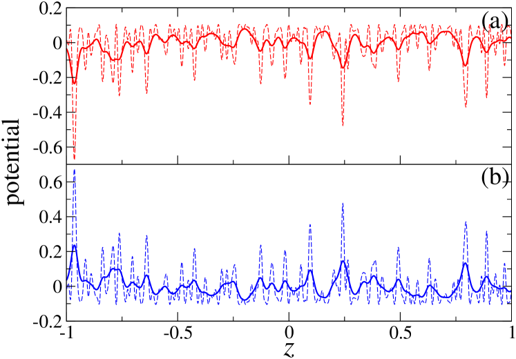
Figure 1: Dashed lines: bare potential $V(z)$, solid lines: convoluted potential, i.e. $\int dz^{\prime}V(z^{\prime})|\phi_{0}(z^{\prime}-z)|^{2}/N$. Panel (a) for the bare potential amplitude $V_{0}=+0.1$ (red detuned laser case), panel (b) for $V_{0}=-0.1$ (blue detuned laser case). The correlation length of the bare potential is $\sigma_{0}=0.28\xi$ where $\xi=0.02$.

Any disordered potential is completely characterized by its correlation functions $\overline{V(z_{1})\dots V(z_{n})}$ where the overbar denotes an ensemble average over disorder realizations. The average potential value shifts the origin of energy and can always be set to zero, $\overline{V(z)}=0$. The pair correlator can be written as $\overline{V(z^{\prime})V(z^{\prime}+z)}=V_{0}^{2}C(z/\sigma_{0})$, where $V_{0}$ measures the potential strength, and $\sigma_{0}$ the spatial correlation length. For a gaussian random process, higher order correlation functions are simple functions of the average and the pair correlator. This is no longer the case for non-gaussian potentials that require to specify also higher-order correlations.

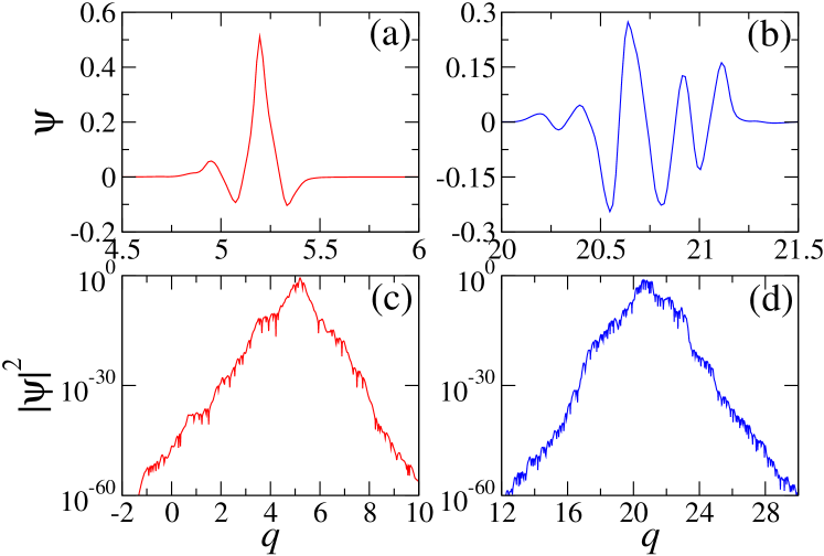
Figure 2: Panels (a) and (b): eigenstates of the CM of a bright soliton; panels (c) and (d): corresponding probability density in log scale. The eigenstates correspond to the CM momentum $P_{q}\approx 10$. The red detuned laser case is shown in (a) and (c) while the blue detuned one in (b) and (d). The inverse localization length is $\gamma=23\pm 3$ (red detuned case) and $\gamma=16.5\pm 0.6$ (blue detuned case). The parameters of the potentials are the same as in Fig. 1.

An optical speckle potential is a good example of such a non-gaussian behaviour. At fixed detuning, the potential features either random peaks (the “blue-detuned” case) or wells (“red-detuned”). Even after shifting to $\overline{V(z)}=0$, the potential distribution is asymmetric (compare Fig. 1), and the importance of odd moments can be probed experimentally by comparing the blue- and red-detuned cases for fixed amplitude $|V_{0}|$. The latter is determined by the laser strength, and we will use $|V_{0}|=8\cdot 10^{-5}|\mu|=0.1$ in the following. The bare speckle potential has the pair correlation function $C(y)=[\sin(y)/y]^{2}$, with a correlation length that can be as short as $0.28\,\mu$m Billy2008 or $\sigma_{0}=0.0056$ in our units. We shall use this value in the following. The CM of the soliton feels, however, not the bare potential, but rather its convolution with the soliton shape, see Eq. (80). The convoluted effective potential $\int dz^{\prime}V(z^{\prime})|\phi_{0}(z^{\prime}-z)|^{2}/N$ (the $N$ factor in the denominator is due to the normalization of $\phi_{0}$) is also shown in Fig. 1. While the convolution makes the potential smoother it is apparent that it remains quite asymmetric, thus we may expect that the non-gaussian character (in particular non-vanishing odd moments) shows up in the properties of the system. For that reason we compare the results for both red- and blue- detuned potential of similar amplitude.

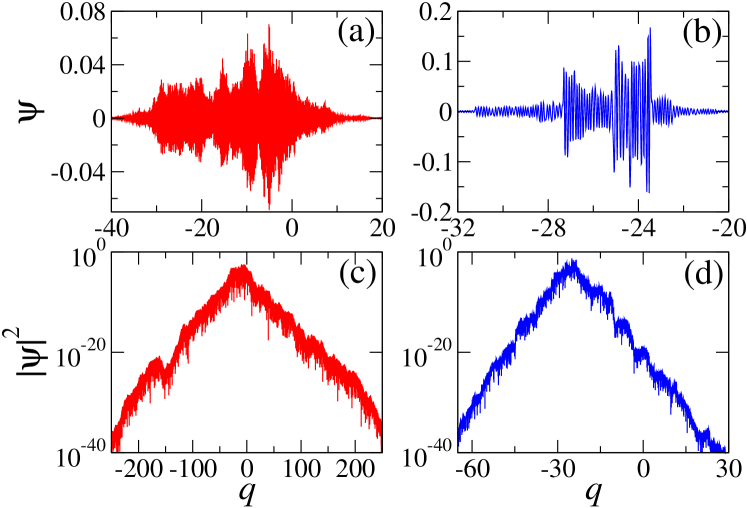
Figure 3: Panels (a) and (b): eigenstates of the CM of soliton; panels (c) and (d): corresponding probability density in log scale. The eigenstates correspond to the CM momentum $P_{q}\approx 50$. The red detuned laser case is shown in (a) and (c) while the blue detuned one in (b) and (d). The inverse localization length is $\gamma=0.27\pm 0.03$ (red detuned case) and $\gamma=1.8\pm 0.1$ (blue detuned case). The parameters of the potentials are the same than in Fig. 1.

The generic properties of Anderson localization in 1D vantiggelen1999 allow us to expect that all the eigenstates of (80) are exponentially localized, i.e., have a typical shape with the overall envelope

$$|\Psi|^{2}\propto\exp\left[-\gamma(P_{q})|q-q_{0}|\right],$$ (81)

with $q_{0}$ being the mean position while $\gamma(P_{q})$ is naturally referred to as the inverse localization length. It depends on the eigenenergy of the state $E$, or writing $P_{q}\approx\sqrt{2NE}$ on the associated momentum $P_{q}$. By diagonalizing the Hamiltonian (80) on a grid, we obtain the wavefunctions that are represented in Fig. 2 and Fig. 3 for two significantly different energies (momenta). Fig. 2 shows the probability densities for the CM of the soliton at relatively low energies, observe that the exponential envelope behaviour is visible over several decades. Due to the tridiagonal form of the diagonalized matrix on the grid, the errors are well under control and the accuracy seems not to be limited by double precision arithmetics. Observe that the inverse localization lengths obtained for red-detuned case and the blue-detuned situation differ significantly, stronger localization is observed for the former case.

The situation is quite different at higher energies as shown in Fig. 3. Observe that now blue-detuned potential leads to a much stronger localization. Of course the inverse localization lengths at high energies are much smaller than those depicted in Fig. 2, in fact, at sufficiently high energies $\gamma(P_{q})$ decays exponentially with $P_{q}$ as observed by us before ours .

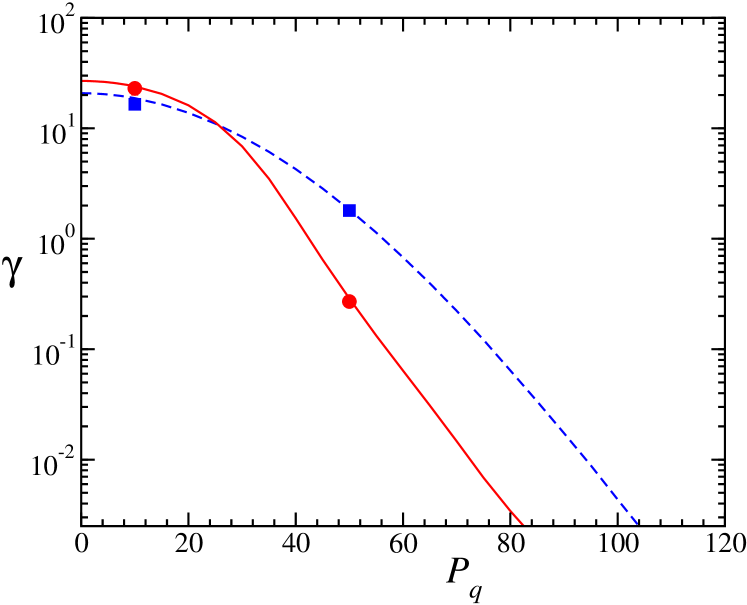
Figure 4: Inverse localization length as a function of the momentum for red-detuned (red-line, solid) and blue-detuned (blue-line, dashed) potentials obtained using the transfer matrix technique. The red dots as well as the blue squares correspond to the wavefunctions shown in Fig. 2 and Fig. 3. Observe the exponential decay of $\gamma$ for sufficiently large $P_{q}$.

The inverse localization lengths shown as lines in Fig. 4 are obtained by a transfer matrix technique MacKinnon1981 and quite nicely agree with values obtained from exact diagonalization. Clearly there is a striking difference between the two cases of red-detuned and blue-detuned potentials exemplifying its non-gaussian character and the importance of higher moments, in particular third moments. This in turn indicates that the application of the celebrated Born approximation vantiggelen1999 ; ours which considers the two lowest moments only is deemed to fail in our case despite the fact that the potential is very weak, smooth and thus, at first glance one could naively expect the Born approximation to perform quite well.

With exponentially localized eigenstates, one can now consider the dynamics, e.g., the spread of an initially localized wavepacket. As shown by us elsewhere ours , one can expect an algebraic localization of such a CM wavepacket. For realistic parameters, localization occurs on a timescale of seconds making the experimental verification of the localization feasible. We refer the reader to ours for details.

V Conclusions

Using the Bogoliubov expansion and treating the zero modes non-perturbatively, we have shown in detail how to obtain the effective quantum Hamiltonian which governs the motion of the center of mass of the bright soliton in a weak and smooth potential without affecting the soliton shape. When this potential is of the disorder type one may expect to observe Anderson localization of the CM motion. The optical speckle potential was considered as a realistic example. It turns out that localization properties of wavefunctions strongly depend on the sign of the potential (red- or blue- detuning). This indicates that, even for a weak potential, applicability of the Born approximation is limited and the quantitative predictions depend on higher correlation functions of the disorder potential. Anderson localization of the CM of a bright soliton should be experimentally observable.

References

- (1) P.W. Anderson, Phys. Rev. 109, 1492 (1958).
- (2) P.A. Lee and T.V. Ramakrishnan, Rev. Mod. Phys. 57, 287 (1985).
- (3) B. van Tiggelen, in Wave Diffusion in Complex Media, lecture notes at Les Houches 1998, edited by J.P. Fouque, NATO Science (Kluwer, Dordrecht, 1999).
- (4) D. Jaksch and P. Zoller, Annals of Physics 315, 52 (2005).
- (5) B. Damski, J. Zakrzewski, L. Santos, P. Zoller, and M. Lewenstein, Phys. Rev. Lett. 91, 080403 (2003).
- (6) J. E. Lye, L. Fallani, M. Modugno, D. Weirsma, C. Fort, M. Inguscio, Phys. Rev. Lett. 95, 070401 (2005).
- (7) C. Fort, L. Fallani, V. Guarrera, J. Lye, M. Modugno, D. S. Wiersma, M. Inguscio Phys. Rev. Lett. 95, 170410 (2005).
- (8) D. Clément, A.F. Varon, M. Hugbart, J.A. Retter, P. Bouyer, L. Sanchez-Palencia, D.M. Gangardt, G.V. Shlyapnikov, and A.Aspect, Phys. Rev. Lett. 95, 170409 (2005).
- (9) T. Schulte, S. Drenkelforth, J. Kruse, W. Ertmer, J. Arlt, K. Sacha, J. Zakrzewski, and M. Lewenstein, Phys. Rev. Lett.95, 170411 (2005).
- (10) T. Schulte, S. Drenkelforth, J. Kruse, R. Tiemeyer, K. Sacha, J. Zakrzewski, M. Lewenstein, W. Ertmer, and J. J. Arlt, New J. Phys. 8, 230 (2006).
- (11) L. Sanchez-Palencia, D. Clément, P. Lugan, P. Bouyer, G. V. Shlyapnikov, and A. Aspect, Phys. Rev. Lett. 98, 210401 (2007).
- (12) P. Lugan, D. Clément, P. Bouyer, A. Aspect, and L. Sanchez-Palencia, Phys. Rev. Lett. 99, 180402 (2007).
- (13) S.E. Skipetrov, A. Minguziz, B.A. van Tiggelen, and B. Shapiro, Phys. Rev. Lett. 100, 165301 (2008).
- (14) J. Billy, V. Josse, Z. C. Zuo, A. Bernard, B. Hambrecht, P. Lugan, D. Clement, L. Sanchez-Palencia, P. Bouyer, A. Aspect, Nature 453, 891 (2008).
- (15) G. Roati, C. D’Errico, L. Fallani, M. Fattori, C. Fort, M. Zaccanti, G. Modugno, M. Modugno, M. Inguscio, Nature 453, 895 (2008).
- (16) S. Aubry and G. André, Ann. Israel Phys. Soc. 3, 133 (1980).
- (17) J.B. McGuire, J. Math. Phys. 5, 622 (1964).
- (18) L. Khaykovich, F. Schreck, G. Ferrari, T. Bourdel, J. Cubizolles, L. D. Carr, Y. Castin, C. Salomon, Science 296, 1290 (2002); K. E. Strecker, G. B. Partridge, A. G. Truscott, R. G. Hulet, Nature 417, 150 (2002).
- (19) S. A. Gredeskul and Y. S. Kivshar, Phys. Rep. 216, 1, (1992).
- (20) Y. Lahini, A. Avidan, F. Pozzi, M. Sorel, R. Morandotti, D. N. Christodoulides, and Y. Silberberg, Phys. Rev. Lett. 100, 013906 (2008); E. N. Tsoy, C. M. de Sterke, F. Kh. Abdullaev, Phys. Rev. A 78, 031803 (2008); E. Akkermans, S. Ghosh, and Z. H. Musslimani, J. Phys. B 41, 045302 (2008).
- (21) K. Sacha, C. A. Müller, D. Delande, and J. Zakrzewski, arXiv:0907.0338.
- (22) V. E. Zakharov and A. B. Shabat, Sov. Phys. JETP 34, 62 (1972).
- (23) Y. Castin and R. Dum, Phys. Rev. A 57, 3008 (1998); Y. Castin, in Les Houches Session LXXII, Coherent atomic matter waves 1999, edited by R. Kaiser, C. Westbrook and F. David, (Springer-Verlag Berlin Heilderberg New York 2001).
- (24) M. Lewenstein and L. You, Phys. Rev. Lett. 77, 3489 (1996).
- (25) J. Dziarmaga, Phys. Rev. A 70, 063616 (2004).
- (26) R. Kanamoto, H. Saito, and M. Ueda, Phys. Rev. A 67, 013608 (2003).
- (27) P. Lugan, A. Aspect, L. Sanchez-Palencia, D. Delande, B. Grémaud, C. A. Müller, C. Miniatura, Phys. Rev. A 80, 023605 (2009).
- (28) A. McKinnon and B. Kramer, Phys. Rev. Lett. 47, 1546 (1981).