Regularity of Cauchy horizons in $S^{2}\times S^{1}$ Gowdy spacetimes

Abstract

We study general $S^{2}\times S^{1}$ Gowdy models with a regular past Cauchy horizon and prove that a second (future) Cauchy horizon exists, provided that a particular conserved quantity $J$ is not zero. We derive an explicit expression for the metric form on the future Cauchy horizon in terms of the initial data on the past horizon and conclude the universal relation $A_{\mathrm{p}}A_{\mathrm{f}}=(8\pi J)^{2}$ where $A_{\mathrm{p}}$ and $A_{\mathrm{f}}$ are the areas of past and future Cauchy horizon respectively.

,

1 Introduction

The well-known singularity theorems by Hawking and Penrose [20] show that cosmological solutions to the Einstein equations generally contain singularities. As discussed by Clarke [13] (see also [14] for a comprehensive overview) there are two types of singularities: (i) curvature singularities, for which components of the Riemann tensor or its $k$th derivatives are irregular (e.g. unbounded), and (ii) quasiregular singularities, which are associated with peculiarities in the topology of space-time (e.g. the vertex of a cone), although the local geometry is well behaved. In addition, the curvature singularities are divided up into scalar singularities (for which some curvature invariants are badly behaved) and nonscalar singularities (for which arbitrarily large or irregular tidal forces occur). The singularity theorems mentioned above provide, however, in general no information about the specific type of singularity — they make statements solely about causal geodesic incompleteness. This lack of knowledge concerning the specific nature of the singular structure is the reason for many open outstanding problems in general relativity, including the strong cosmic censorship conjecture and the BKL conjecture (see [1] for an overview).

A major motivation for the study of Gowdy spacetimes as relatively simple, but non-trivial inhomogeneous cosmological models results from the desire to understand the mathematical and physical properties of such cosmological singularities. The Gowdy cosmologies, first studied in [17, 18], are characterized by an Abelian isometry group $U(1)\times U(1)$ with spacelike group orbits, i.e. these spacetimes possess two associated spacelike and commuting Killing vector fields $\xi$ and $\eta$. Moreover, the definition of Gowdy spacetimes includes that the twist constants $\epsilon_{\alpha\beta\gamma\delta}\xi^{\alpha}\eta^{\beta}\nabla^{\gamma}\xi^{\delta}$and $\epsilon_{\alpha\beta\gamma\delta}\xi^{\alpha}\eta^{\beta}\nabla^{\gamma}\eta^{\delta}$ (which are constant as a consequence of the field equations) are zero.

For compact, connected, orientable and smooth three manifolds, the corresponding spatial topology must be either $T^{3}$, $S^{3}$, $S^{2}\times S^{1}$ or $L(p,q)$, cf. [18] (see also [26, 30, 15]). Note that the universal cover of the lens space $L(p,q)$ is $S^{3}$ and hence this case needs not be treated separately, see references in [10].

In the $T^{3}$-case, global existence in time with respect to the areal foliation time $t$ was proved by Moncrief [25]. Moreover, he has shown that the trace of the second fundamental form blows up uniformly on the hypersurfaces $t=\textrm{constant}$ in the limit $t\to 0$. As a consequence, the solutions do not permit a globally hyperbolic extension beyond the time $t=0$. However, to date it has not been clarified whether the solutions are extendible (as non-globally hyperbolic $C^{2}$-solutions) or are generically subject to curvature singularities at $t=0$.

Although global existence of solutions inside the “Gowdy square” (i.e. for $0<t<\pi$, cf. Fig. 1 below) was shown by Chruściel for $S^{2}\times S^{1}$ and $S^{3}$ topology, see Thm. 6.3 in [10], it is still an open question whether globally hyperbolic extensions beyond the hypersurfaces $t=0$ or $t=\pi$ exist. It is expected that these hypersurfaces contain either curvature singularities or Cauchy horizons; the theorem in [10] however does not in fact exclude the possibility that these are merely coordinate singularities.

For polarized Gowdy models, where the Killing vector fields can be chosen to be orthogonal everywhere, the nature of the singularities for all possible spatial topologies has been studied in [22, 11]. In particular, strong cosmic censorship and a version of the BKL conjecture have been proved. Investigations of singularities in the unpolarized case for $T^{3}$ topology can be found in [5, 24, 32, 33].

For unpolarized $S^{3}$ or $S^{2}\times S^{1}$ Gowdy spacetimes not many results on singularities (strong cosmic censorship, BKL conjecture, Gowdy spikes) are known. Particular singular solutions have been constructed with Fuchsian techniques in [34]. Moreover, numerical studies indicate that the behavior near singularities and the appearance of spikes are similar to the $T^{3}$-case [16, 6, 7].

In this paper, we study general (unpolarized or polarized) $S^{2}\times S^{1}$ Gowdy models with a regular Cauchy horizon (with $S^{2}\times S^{1}$ topology) at $t=0$ (cf. Fig. 1) and assume that the spacetime is regular (precise regularity requirements are given below) at this horizon as well as in a neighborhood. As mentioned above, a theorem by Chruściel [10] implies then that the metric is regular for all $t<\pi$, i.e. excluding only the future hypersurface $t=\pi$. With the methods utilized in this paper we are able to provide the missing piece, i.e. we prove that under our regularity assumptions the existence of a regular second (future) Cauchy horizon ${\mathcal{H}_{\mathrm{f}}}$ (at $t=\pi$) is implied, provided that a particular conserved quantity $J$ is not zero. Moreover, we derive an explicit expression for the metric form on the future Cauchy horizon in terms of the initial data on the past horizon. From this explicit formula, the universal relation $A_{\mathrm{p}}A_{\mathrm{f}}=(8\pi J)^{2}$ between the areas $A_{\mathrm{p}},A_{\mathrm{f}}$ of past and future Cauchy horizons and the above mentioned conserved quantity $J$ can be concluded.

The proofs of these statements can be found by relating any $S^{2}\times S^{1}$ Gowdy model to a corresponding axisymmetric and stationary black hole solution (with possibly non-pure vacuum exterior, e.g. with surrounding matter), considered between outer event and inner Cauchy horizon. Note that the region between these horizons is regular hyperbolic, i.e. the Einstein equations are hyperbolic PDEs in an appropriate gauge with coordinates adapted to the Killing vectors, see [2, 3, 23]. (The Kerr metric is an explicitly known solution of these PDEs, see [31].) As a consequence, the results on the regularity of the interior of such black holes and existence of regular Cauchy horizons inside the black holes obtained in [2, 3, 23] can be carried over to Gowdy spacetimes.

The results in [2] were found by utilizing a particular soliton method — the so-called Bäcklund transformation. Making use of the theorem by Chruściel mentioned earlier, it was possible to show that a regular Cauchy horizon inside the black hole always exists, provided that the angular momentum of the black hole does not vanish. (The above quantity $J$ is the Gowdy counterpart of the angular momentum.)

In [3, 23] these results have been generalized to the case in which an additional Maxwell field is considered. The corresponding technique, that is the inverse scattering method, again comes from soliton theory and permits the reconstruction of the field quantities along the entire boundary of the Gowdy square. Hereby, an associated linear matrix problem is analyzed, whose integrability conditions are equivalent to the non-linear field equations in axisymmetry and stationarity. Note that in this article we restrict ourselves to the pure Einstein case (without Maxwell field) and refer the reader to [3, 23] for results valid in full Einstein-Maxwell theory.

We start by introducing appropriate coordinates, adapted to the description of regular axes and Cauchy horizons at the boundaries of the Gowdy square, see Sec. 2. Moreover, we revisit the complex Ernst formulation of the field equations and corresponding boundary conditions and introduce the conserved quantity $J$ in question. In this formulation we can translate the results of [2, 3, 23] and obtain the metric on the future Cauchy horizon in terms of initial data on the past horizon, see Sec. 3. As another consequence we arrive at the above equation relating $A_{\mathrm{p}},A_{\mathrm{f}}$ and $J$, see Sec. 4. Finally, in Sec. 5 we conclude with a discussion of our results.

2 Coordinates and Einstein equations

2.1 Coordinate system, Einstein equations and regularity requirements

We introduce suitable coordinates and metric functions by adopting our notation from [16]. Accordingly, we write the Gowdy line element in the form

$$\mathrm{d}s^{2}=\mathrm{e}^{M}(-\mathrm{d}t^{2}+\mathrm{d}\theta^{2})+\sin t\sin\theta\left[\mathrm{e}^{L}(\mathrm{d}\varphi+Q\mathrm{d}\delta)^{2}+\mathrm{e}^{-L}\mathrm{d}\delta^{2}\right],$$ (1)

where the metric functions $M$, $L$ and $Q$ depend on $t$ and $\theta$ alone. In these coordinates, the two Killing vectors are given by

$$\eta=\frac{\partial}{\partial\varphi},\qquad\xi=\frac{\partial}{\partial\delta}.$$ (2)

As mentioned in Sec. 1, any $S^{2}\times S^{1}$ Gowdy model can be related to the spacetime portion between outer event and inner Cauchy horizon of an appropriate axisymmetric and stationary black hole solution. Black hole spacetimes of this kind have been studied by Carter [8] and Bardeen [4]. Among other issues they discussed conditions for regular horizons. In this paper we adopt their regularity arguments for our study of Gowdy spacetimes. Accordingly we rewrite the line element (1) in the form

$$\mathrm{d}s^{2}=\mathrm{e}^{M}(-\mathrm{d}t^{2}+\mathrm{d}\theta^{2})+\mathrm{e}^{u}\sin^{2}\!\theta(\mathrm{d}\varphi+Q\mathrm{d}\delta)^{2}+\mathrm{e}^{-u}\sin^{2}\!t\,\mathrm{d}\delta^{2}$$ (3)

where

$$u=\ln\sin t-\ln\sin\theta+L.$$ (4)

Now, at a regular horizon (clear statements about the type of regularity follow below) the metric functions $M,Q$ and $u$ are regular, meaning that $L$ possesses a specific irregular behavior there.

At this point, some remarks about the specific regularity requirements needed in our investigation are necessary. A crucial role is played by a theorem of Chruściel (Theorem 6.3 in [10]) which provides us with the essential regularity information valid in the interior of the Gowdy square. In this theorem it is assumed that initial data are given on an interior Cauchy slice, described by $t=\mbox{constant}=t_{0},$ $0<t_{0}<\pi$. These data are supposed to consist of (i) metric potentials that are $H^{k}$-functions of $\theta$ and (ii) first time derivatives that are $H^{k-1}$-functions of $\theta$ (with $k\geq 3$). Here $H^{k}$ denotes the Sobolev space $W^{k,2}$ that contains all functions for which both the function and its weak derivatives up to the order $k$ are in $L^{2}$. With these assumptions the theorem by Chruściel guarantees the existence of a unique continuation of the given initial data for which the metric is $H^{k}$ on all future spatial slices $t=\mbox{constant}$ with $t_{0}<t<\pi$, i.e. only the future boundary $t=\pi$ of the Gowdy square is excluded. (Note that Theorem 6.3 as formulated in [10] assumes the metric to be smooth. However, this condition can be relaxed considerably to the assumption of $H^{k}$ spaces [12].)

Now, for the applicability of our soliton methods it is essential that the metric potentials in (3) possess $C^{2}$-regularity. Therefore, in order to apply both Chruściel’s theorem and the soliton methods, we need to require that the metric potentials $M$, $u$, $Q$ be $H^{4}$-functions and the time derivatives $H^{3}$-functions of $\theta$ on all slices $t=\textrm{constant}$ in a neighborhood of the horizon ${\mathcal{H}_{\mathrm{p}}}$, see Fig. 1. Then Chruściel’s theorem ensures the existence of an $H^{4}$-regular continuation which implies (via Sobolev embeddings and the validity of the Einstein equations) that the metric potentials $M$, $u$, $Q$ are $C^{2}$-functions of $t$ and $\theta$ for ($t,\theta)\in(0,\pi)\times[0,\pi]$, i.e. in the entire Gowdy square with the exception of the two horizons ${\mathcal{H}_{\mathrm{p}}}\,(t=0)$ and ${\mathcal{H}_{\mathrm{f}}}\,(t=\pi)$. Now, in accordance with Carter’s and Bardeen’s arguments concerning regularity at the horizon, we require that this $C^{2}$-regularity holds also for $t=0$, i.e. we assume in this manner a specifically regular past horizon ${\mathcal{H}_{\mathrm{p}}}$.

As mentioned above, these requirements allow us to utilize our soliton methods at ${\mathcal{H}_{\mathrm{p}}}$. Since ${\mathcal{H}_{\mathrm{p}}}$ is a degenerate boundary surface of the interior hyperbolic region, the study of the Einstein equations provides us with specific relations that permit the identification of an appropriate set of initial data of the hyperbolic problem at the past Cauchy horizon ${\mathcal{H}_{\mathrm{p}}}$.

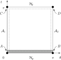
Figure 1: The Gowdy square. We assume a $H^{4}$-regular metric and $H^{3}$-regular time derivatives on all slices $t=\textrm{constant}$ in a neighborhood (gray region) of the past Cauchy horizon (${\mathcal{H}_{\mathrm{p}}}:t=0$) and find by virtue of the results in [2], that then the metric is $H^{4}$-regular on all future slices $t=\textrm{constant}$, $0\leq t\leq\pi$ (unless the quantity $J$ introduced in (25) is zero). In particular, a $H^{4}$-regular future Cauchy horizon (${\mathcal{H}_{\mathrm{f}}}:t=\pi$) exists.

For the line element (3), the Einstein equations read as follows:

$$-u_{,tt}-\cot t\,u_{,t}+u_{,\theta\theta}+\cot\theta\,u_{,\theta}=2-\frac{\sin^{2}\theta}{\sin^{2}t}\mathrm{e}^{2u}\left(Q_{,t}^{2}-Q_{,\theta}^{2}\right),$$ (5)

$$-Q_{,tt}+\cot t\,Q_{,t}+Q_{,\theta\theta}+3\cot\theta\,Q_{,\theta}-2(u_{,t}Q_{,t}-u_{,\theta}Q_{,\theta})=0,$$ (6)

$$-M_{,tt}+M_{,\theta\theta}-\frac{1}{2}u_{,t}(u_{,t}-2\cot t)+\frac{1}{2}u_{,\theta}(u_{,\theta}+2\cot\theta)-\frac{1}{2}\frac{\sin^{2}\theta}{\sin^{2}t}\mathrm{e}^{2u}\left(Q_{,t}^{2}-Q_{,\theta}^{2}\right)=0.$$ (7)

Alternatively to (7), the metric potential $M$ can also be calculated from the first order field equations

$$(\cos^{2}t-\cos^{2}\theta)M_{,t} = \frac{1}{2}\mathrm{e}^{2u}\frac{\sin^{3}\theta}{\sin t}\left[\cos t\sin\theta(Q_{,t}^{2}+Q_{,\theta}^{2})-2\sin t\cos\theta\,Q_{,t}Q_{,\theta}\right]$$ (8)

$$+\frac{1}{2}\sin t\sin\theta\left[\cos t\sin\theta(u_{,t}^{2}+u_{,\theta}^{2})-2\sin t\cos\theta\,u_{,t}u_{,\theta}\right]$$

$$+(2\cos^{2}t\cos^{2}\theta-\cos^{2}t-\cos^{2}\theta)u_{,t}$$

$$+2\sin t\cos t\sin\theta\cos\theta(u_{,\theta}-\tan\theta),$$

$$(\cos^{2}t-\cos^{2}\theta)M_{,\theta} = -\frac{1}{2}\mathrm{e}^{2u}\frac{\sin^{3}\theta}{\sin t}\left[\sin t\cos\theta(Q_{,t}^{2}+Q_{,\theta}^{2})-2\cos t\sin\theta\,Q_{,t}Q_{,\theta}\right]$$ (9)

$$-\frac{1}{2}\sin t\sin\theta\left[\sin t\cos\theta(u_{,t}^{2}+u_{,\theta}^{2})-2\cos t\sin\theta\,u_{,t}u_{,\theta}\right]$$

$$+2\sin t\cos t\sin\theta\cos\theta(u_{,t}+\tan t)$$

$$+(2\cos^{2}t\cos^{2}\theta-\cos^{2}t-\cos^{2}\theta)u_{,\theta}.$$

These expressions tell us that (see A for a detailed derivation)

$$M_{,t}=Q_{,t}=u_{,t}=0\,,\quad Q=Q_{\mathrm{p}}=\mbox{constant}\,,\quad M+u=\textrm{constant}$$ (10)

holds on ${\mathcal{H}_{\mathrm{p}}}$. As the $t$-derivatives of all metric functions vanish identically at ${\mathcal{H}_{\mathrm{p}}}$, a complete set of initial data at ${\mathcal{H}_{\mathrm{p}}}$ consists of

$$Q=Q_{\mathrm{p}}\in\mathds{R},\quad u\in H^{4},\quad Q_{,tt}\in H^{2},$$ (11)

where $Q_{,tt}$ is in $H^{2}$ as a consequence of the regularity assumptions discussed above. Note that among the second $t$-derivatives only $Q_{,tt}$ can be chosen freely since the values of $M_{,tt}$ as well as $u_{,tt}$ are then fixed, as again the study of the field equations (5)-(7) near ${\mathcal{H}_{\mathrm{p}}}$ reveals. Similarly, $M$ is also fixed on ${\mathcal{H}_{\mathrm{p}}}$ by the choice of the data in (11).

It turns out that the constant $Q_{\mathrm{p}}$ is a gauge degree of freedom. This results from the fact that the line element (1) is invariant under the coordinate change

$$\Sigma:(t,\theta,\varphi,\delta)\mapsto\Sigma^{\prime}:(t,\theta,\varphi^{\prime}=\varphi-\Omega\delta,\delta),$$ (12)

leading to $Q_{\mathrm{p}}^{\prime}=Q_{\mathrm{p}}+\Omega$ in the new coordinates . We use this freedom in order to exclude two specific values, namely $Q_{\mathrm{p}}=0$ and $Q_{\mathrm{p}}=1/J$, where $J$ is the already mentioned conserved quantity that will be introduced in (26). This exclusion becomes necessary since the analysis carried out below breaks down if $Q_{\mathrm{p}}$ takes one of these values.

We note further that as another consequence of our regularity requirements, the following axis condition holds at least in a neighborhood of the points $A$ and $B$ (cf. Fig. 1):

$$\mathcal{A}_{1/2}:\qquad M=u.$$ (13)

Moreover, at these points $A,B$ we have (see A)

$$M_{A}=M_{B}=u_{A}=u_{B}.$$ (14)

Note that solutions which are also $C^{2}$-regular up to and including ${\mathcal{H}_{\mathrm{f}}}$ satisfy corresponding conditions at the points $C$ and $D$.

2.2 The Ernst equation

In order to introduce the Ernst formulation of the Einstein equations, we define the complex Ernst potential

$$\mathcal{E}(t,\theta)=f(t,\theta)+\mathrm{i}b(t,\theta),$$ (15)

where the real part $f$ is given by

$$f:=-\xi_{i}\xi^{i}=-\mathrm{e}^{-u}\sin^{2}\!t-Q^{2}\mathrm{e}^{u}\sin^{2}\!\theta$$ (16)

and the imaginary part $b$ is defined in terms of a potential $a$,

$$a:=\frac{\xi^{i}\eta_{i}}{\xi^{j}\xi_{j}}=-\frac{Q}{f}\mathrm{e}^{u}\sin^{2}\!\theta,$$ (17)

via

$$a_{,t}=\frac{1}{f^{2}}\sin t\sin\theta\,b_{,\theta},\qquad a_{,\theta}=\frac{1}{f^{2}}\sin t\sin\theta\,b_{,t}.$$ (18)

In this formulation, the vacuum Einstein equations are equivalent to the Ernst equation

$$\Re(\mathcal{E})\left(-\mathcal{E}_{,tt}-\cot t\,\mathcal{E}_{,t}+\mathcal{E}_{,\theta\theta}+\cot\theta\,\mathcal{E}_{,\theta}\right)=-\mathcal{E}_{,t}^{2}+\mathcal{E}_{,\theta}^{2},$$ (19)

where $\Re(\mathcal{E})$ denotes the real part of $\mathcal{E}$. As a consequence of (19), the integrability condition $a_{,t\theta}=a_{,\theta t}$ of the system (18) is satisfied such that $a$ may be calculated from (18) using $\mathcal{E}$. Moreover, given $a$ and $\mathcal{E}$ we can use (16) and (17) to obtain the metric functions $u$ and $Q$. Finally, the potential $M$ may be calculated from

$$M_{,t} = -\frac{f_{,t}}{f}+\frac{1}{2f^{2}}\frac{\sin t\sin\theta}{\cos^{2}\!t-\cos^{2}\!\theta}\Big{[}\cos t\sin\theta\left(f_{,t}^{2}+f_{,\theta}^{2}+b_{,t}^{2}+b_{,\theta}^{2}\right)$$ (20)

$$-2\sin t\cos\theta\left(f_{,t}f_{,\theta}+b_{,t}b_{,\theta}\right)-4f^{2}\frac{\cos t}{\sin\theta}\Big{]},$$

$$M_{,\theta} = -\frac{f_{,\theta}}{f}-\frac{1}{2f^{2}}\frac{\sin t\sin\theta}{\cos^{2}\!t-\cos^{2}\!\theta}\Big{[}\sin t\cos\theta\left(f_{,t}^{2}+f_{,\theta}^{2}+b_{,t}^{2}+b_{,\theta}^{2}\right)$$ (21)

$$-2\cos t\sin\theta\left(f_{,t}f_{,\theta}+b_{,t}b_{,\theta}\right)-4f^{2}\frac{\cos\theta}{\sin t}\Big{]}$$

since the Ernst equation (19) also ensures the integrability condition $M_{,t\theta}=M_{,\theta t}$.

As for the potentials introduced in Sec. 2.1 we conclude axis conditions which hold at least in a neighborhood of the points $A$ and $B$ (cf. Fig. 1):

$$\mathcal{A}_{1/2}:\qquad\mathcal{E}_{,\theta}=0,\quad a=0.$$ (22)

Moreover, at the points $A,B$ we have $f=0$. Again, solutions which are also $H^{4}$-regular on ${\mathcal{H}_{\mathrm{f}}}$ satisfy corresponding conditions at the points $C$ and $D$.

It turns out that initial data $\mathcal{E}_{\mathrm{p}}(\theta)\equiv\mathcal{E}(0,\theta)=f_{\mathrm{p}}(\theta)+\mathrm{i}b_{\mathrm{p}}(\theta)$ of the Ernst potential are equivalent to the inital data set consisting of $u$, $Q=Q_{\mathrm{p}}$, $Q_{,tt}$ at ${\mathcal{H}_{\mathrm{p}}}$. Both sets are related via

$$f_{\mathrm{p}} = -Q_{\mathrm{p}}^{2}\mathrm{e}^{u(0,\theta)}\sin^{2}\!\theta,$$ (23)

$$b_{\mathrm{p}} = b_{A}+2Q_{\mathrm{p}}(\cos\theta-1)-Q_{\mathrm{p}}^{2}\int_{0}^{\theta}\mathrm{e}^{2u(0,\theta^{\prime})}Q_{,tt}(0,\theta^{\prime})\sin^{3}\!\theta^{\prime}\,\mathrm{d}\theta^{\prime},$$ (24)

where $b_{A}=b(0,0)$ is an arbitrary integration constant.

2.3 Conserved quantities

As a consequence of the symmetries of the Gowdy metric, there exist conserved quantities, i.e. integrals with respect to $\theta$ that are independent of the coordinate time $t$. One of them is $J$, defined by

$$J:=-\frac{1}{8}\int_{0}^{\pi}\frac{Q_{,t}(t,\theta)}{\sin t}\,\mathrm{e}^{2u(t,\theta)}\sin^{3}\!\theta\,\mathrm{d}\theta=\mbox{constant}.$$ (25)

As for the black hole angular momentum in the corresponding axisymmetric and stationary black hole spacetimes (cf. discussion at the end of Sec. 1), this quantity determines whether or not a regular future Cauchy horizon exists. In fact, it exists if and only if $J\neq 0$ holds. Note that $J$ vanishes in polarized Gowdy models, where we have $Q_{,t}\equiv 0$.

It turns out that $J$ can be read off directly from the Ernst potential and its second $\theta$-derivative at the points $A$ and $B$ on ${\mathcal{H}_{\mathrm{p}}}$ (see Fig. 1),

$$J=-\frac{1}{8Q_{\mathrm{p}}^{2}}(b_{A}-b_{B}-4Q_{\mathrm{p}}),\quad Q_{\mathrm{p}}=-\frac{1}{2}b_{,\theta\theta}|_{A}$$ (26)

where

$$b_{B}=b(t=0,\theta=\pi).$$

A detailed derivation of these formulas can be found in [23].

3 Potentials on $\mathcal{A}_{1}$, $\mathcal{A}_{2}$, and ${\mathcal{H}_{\mathrm{f}}}$

3.1 Ernst potential

In the previous sections we have derived a formulation which permits the direct translation to the situation in which the hyperbolic region inside the event horizon of an axisymmetric and stationary black hole (with possibly non-pure vacuum exterior, e.g. with surrounding matter) is considered, as was done in [2, 3, 23].

In [2] it has been demonstrated that a specific soliton method (the Bäcklund transformation, see B) can be used to write the Ernst potential $\mathcal{E}$ in terms of another Ernst potential $\mathcal{E}_{0}$ which corresponds to a spacetime without a black hole, but with a completely regular central vacuum region. Interestingly, the potential $\mathcal{E}_{0}=\mathcal{E}_{0}(t,\theta)$ possesses specific symmetry conditions which translate here into

$$\begin{array}[]{lcll}\mathcal{E}_{0}(t,0)&=&\mathcal{E}_{0}(0,t)&\quad\mbox{potential at $\mathcal{A}_{1}$},\\[5.69054pt] \mathcal{E}_{0}(t,\pi)&=&\mathcal{E}_{0}(0,\pi-t)&\quad\mbox{potential at $\mathcal{A}_{2}$},\\[5.69054pt] \mathcal{E}_{0}(\pi,\theta)&=&\mathcal{E}_{0}(0,\pi-\theta)&\quad\mbox{potential at ${\mathcal{H}_{\mathrm{f}}}$}.\end{array}$$

Hence the potential values at the boundaries $\mathcal{A}_{1}$, $\mathcal{A}_{2}$ and ${\mathcal{H}_{\mathrm{f}}}$ are given explicitly in terms of those at ${\mathcal{H}_{\mathrm{p}}}$. Now the Bäcklund transformation carries these dependencies over to the corresponding original Ernst potential $\mathcal{E}$, i.e. we obtain $\mathcal{E}$ at $\mathcal{A}_{1}$, $\mathcal{A}_{2}$ and ${\mathcal{H}_{\mathrm{f}}}$ completely in terms of the initial data at ${\mathcal{H}_{\mathrm{p}}}$.

An alternative approach (see [3, 23]) uses the inverse scattering method. In these papers the potentials on $\mathcal{A}_{1}$, $\mathcal{A}_{2}$ and ${\mathcal{H}_{\mathrm{f}}}$ were obtained from the investigation of an associated linear matrix problem. The integrability conditions of this matrix problem are equivalent to the non-linear field equations, see B. We may carry the corresponding procedure over to our considerations of Gowdy spacetimes. Accordingly we are able to perform an explicit integration of the linear problem along the boundaries of the Gowdy square. Since the resulting solution is closely related to the Ernst potential, it provides us with the desired expressions between the metric quantities on the four boundaries of the Gowdy square.

Note that in both approaches the axes $\mathcal{A}_{1}$ and $\mathcal{A}_{2}$ are considered first. Starting at ${\mathcal{H}_{\mathrm{p}}}$ and using the theorem by Chruściel [10], which ensures $H^{4}$-regularity of the metric inside the Gowdy square (i.e. excluding only ${\mathcal{H}_{\mathrm{f}}}$), we derive first the Ernst potentials at $\mathcal{A}_{1}$ and $\mathcal{A}_{2}$ in terms of the values at ${\mathcal{H}_{\mathrm{p}}}$. It turns out that for $J\neq 0$ these formulas can be extended continuously to the points $C$ and $D$ at which $\mathcal{A}_{1}$ and $\mathcal{A}_{2}$ meet ${\mathcal{H}_{\mathrm{f}}}$ (cf. Fig. 1). Moreover, with the values at $C$ and $D$ it is possible to proceed to ${\mathcal{H}_{\mathrm{f}}}$, and in this way we eventually find an Ernst potential which is continuous along the entire boundary of the Gowdy square. As the theorem by Chruściel ensures unique solvability of the Einstein equations inside the Gowdy square, we conclude that the $H^{4}$-regularity of the Ernst potential holds up to and including ${\mathcal{H}_{\mathrm{f}}}$ which therefore turns out to be an $H^{4}$-regular future Cauchy horizon.

The resulting expressions of the Ernst potentials at the boundaries $\mathcal{A}_{1}$, $\mathcal{A}_{2}$ and ${\mathcal{H}_{\mathrm{f}}}$ read

$$\mathcal{A}_{1}: \quad\mathcal{E}_{1}(x):=\mathcal{E}(t=\arccos x,\theta=0)\hskip 17.64069pt=\frac{\mathrm{i}[b_{A}-2Q_{\mathrm{p}}(x-1)]\mathcal{E}_{\mathrm{p}}(x)+b_{A}^{2}}{\mathcal{E}_{\mathrm{p}}(x)-\mathrm{i}[b_{A}+2Q_{\mathrm{p}}(x-1)]},$$ (27)

$$\mathcal{A}_{2}: \quad\mathcal{E}_{2}(x):=\mathcal{E}(t=\arccos(-x),\theta=\pi)=\frac{\mathrm{i}[b_{B}-2Q_{\mathrm{p}}(x+1)]\mathcal{E}_{\mathrm{p}}(x)+b_{B}^{2}}{\mathcal{E}_{\mathrm{p}}(x)-\mathrm{i}[b_{B}+2Q_{\mathrm{p}}(x+1)]},$$ (28)

$${\mathcal{H}_{\mathrm{f}}}: \quad\mathcal{E}_{\mathrm{f}}(x):=\mathcal{E}(t=\pi,\theta=\arccos(-x))\hskip 1.90633pt=\frac{a_{1}(x)\mathcal{E}_{\mathrm{p}}(x)+a_{2}(x)}{b_{1}(x)\mathcal{E}_{\mathrm{p}}(x)+b_{2}(x)},$$ (29)

where

$$\mathcal{E}_{\mathrm{p}}(x):=\mathcal{E}(t=0,\theta=\arccos x)$$ (30)

denotes the Ernst potential on ${\mathcal{H}_{\mathrm{p}}}$ and $a_{1}$, $a_{2}$, $b_{1}$, and $b_{2}$ in (29) are polynomials in $x$, defined by

$$a_{1} = \mathrm{i}\big{[}16Q_{\mathrm{p}}^{2}(1-x^{2})+8Q_{\mathrm{p}}(b_{A}(x+1)+b_{B}(x-1))$$ (31)

$$\qquad+(b_{A}-b_{B})(b_{A}(x-1)^{2}-b_{B}(x+1)^{2})\big{]},$$

$$a_{2} = 8Q_{\mathrm{p}}[b_{A}^{2}(x+1)+b_{B}^{2}(x-1)]-4b_{A}b_{B}(b_{A}-b_{B})x,$$ (32)

$$b_{1} = 4(4Q_{\mathrm{p}}+b_{B}-b_{A})x,$$ (33)

$$b_{2} = \mathrm{i}\big{[}4Q_{\mathrm{p}}(1-x^{2})-b_{A}(1+x)^{2}+b_{B}(1-x)^{2}\big{]}(4Q_{\mathrm{p}}+b_{B}-b_{A}).$$ (34)

A discussion of (29) shows that $\mathcal{E}_{\mathrm{f}}$ is indeed always regular provided that the black hole angular momentum does not vanish, which in turn means that $J\neq 0$, cf. (25). In order to prove this statement, we first note that both numerator and denominator on the right hand side of (29) are completely regular functions in terms of $x$, since $a_{1}$, $a_{2}$, $b_{1}$, $b_{2}$ are polynomials in $x$ and the initial function $\mathcal{E}_{\mathrm{p}}$ is regular by assumption. Hence, an irregular behavior of the potential $\mathcal{E}_{\mathrm{f}}$ could only be caused by a zero of the denominator. Consequently, we investigate whether the equation

$$b_{1}(x)\mathcal{E}_{\mathrm{p}}(x)+b_{2}(x)=0$$ (35)

has solutions $x\in[-1,1]$. The real part of (35) is given by

$$4x(4Q_{\mathrm{p}}+b_{B}-b_{A})f_{\mathrm{p}}(x)=0.$$ (36)

Using (23) and (26) together with our gauge $Q_{\mathrm{p}}\neq 0$ and the assumption $J\neq 0$ we find that (36) has exactly the three zeros, $x=-1$, $x=0$ and $x=1$ (corresponding to $\theta=\pi$, $\theta=\pi/2$ and $\theta=0$). Now, for $x=0$ the imaginary part of (35) does not vanish, whereas for $x=\pm 1$ it does. Thus we find that the only zeros of the denominator in (29) are located at the two axes ($x=\pm 1$). As a matter of fact, the regular numerator of (29) also vanishes at $x=\pm 1$, as can be derived in a similar manner. Consequently, we study the behavior of $\mathcal{E}_{\mathrm{f}}$ for $x=\pm 1$ in terms of the rule by L’Hôpital. As both numerator and denominator in (29) have non-vanishing values of the derivative with respect to $x$ for $x=\pm 1$, we conclude that the Ernst potential is regular everywhere whenever $J\neq 0$ holds.

Consider now the limit $J\to 0$ for which the expression

$$4Q_{\mathrm{p}}+b_{B}-b_{A}$$

vanishes, cf. (26). As this term appears as a factor in both $b_{1}$ and $b_{2}$ (cf. (33),(34)), we find that the denominator in (29) vanishes identically. The numerator, however, remains non-zero, which means that Ernst potential diverges on the entire future boundary $t=\pi$, $0\leq\theta\leq\pi$. We conclude that ${\mathcal{H}_{\mathrm{f}}}$ becomes singular in the limit $J\to 0$. This divergent behavior of the Ernst potential corresponds to the formation of a (scalar) curvature singularity at ${\mathcal{H}_{\mathrm{f}}}$. In order to illustrate this property, we calculate the Kretschmann scalar at the point $C$ on ${\mathcal{H}_{\mathrm{f}}}$ (see Fig. 1). Using the axis conditions discussed in Sec. 2 and the Einstein equations, we obtain

$$R_{ijkl}R^{ijkl}|_{C}=12\left[\mathrm{e}^{-2u}(1+2u_{,tt})^{2}-Q_{,tt}^{2}\right]_{C}.$$ (37)

In terms of the Ernst potential, this expression reads (cf. Eq. (40) below)

$$R_{ijkl}R^{ijkl}|_{C}=\frac{1}{3}\left[(f_{,tt}+f_{,tttt})^{2}-(b_{,tt}+b_{,tttt})^{2}\right]_{C}.$$ (38)

Now we can use (27) to derive a formula that contains only the initial data on the past horizon ${\mathcal{H}_{\mathrm{p}}}$. Together with (26) we get

$$R_{ijkl}R^{ijkl}|_{C}=-\frac{3}{256Q_{\mathrm{p}}^{8}J^{6}}\left[(16Q_{\mathrm{p}}^{4}J^{2}-4b_{,xx}Q_{\mathrm{p}}^{2}J-f_{,x}^{2})^{2}-16Q_{\mathrm{p}}^{4}J^{2}(f_{,xx}-2f_{,x})^{2}\right]_{B},$$ (39)

where $x=\cos\theta$. Note that the numerator is well-defined and bounded for our $H^{4}$-regular metric, a fact which is ensured by the validity of the Einstein equations near ${\mathcal{H}_{\mathrm{p}}}$.

Equation (39) indicates that the Kretschmann scalar diverges as $J^{-6}$ in the limit $J\to 0$. In fact, as we choose $Q_{\mathrm{p}}\neq 0$ (see Sec. 2.1), and furthermore $f_{,x}\neq 0$ holds (because $2\pi f_{,x}=-Q_{\mathrm{p}}^{2}A_{\mathrm{p}}$ where $A_{\mathrm{p}}$, $0<A_{\mathrm{p}}<\infty$, is the horizon area of ${\mathcal{H}_{\mathrm{p}}}$, see Sec. 4), we conclude that $f_{,x}^{4}$ is the dominating term in the numerator of (39) for sufficiently small $J$. Hence the Kretschmann scalar indeed diverges as $J^{-6}$ in the limit $J\to 0$.

3.2 Metric potentials

From the Ernst potentials $\mathcal{E}_{1}=f_{1}+\mathrm{i}b_{1}$, $\mathcal{E}_{2}=f_{2}+\mathrm{i}b_{2}$, $\mathcal{E}_{\mathrm{f}}=f_{\mathrm{f}}+\mathrm{i}b_{\mathrm{f}}$ in (27), (28), (29) we may calculate the metric potentials $M$, $Q$ and $u$ on the boundaries of the Gowdy square. Using (16), (17), (18), (10), (13), (14) we obtain

$$\mathcal{A}_{1}: \mathrm{e}^{M_{1}}=\mathrm{e}^{u_{1}}=-\frac{\sin^{2}\!t}{f_{1}},\quad Q_{1}=\frac{b_{1,t}}{2\sin t},$$ (40)

$$\mathcal{A}_{2}: \mathrm{e}^{M_{2}}=\mathrm{e}^{u_{2}}=-\frac{\sin^{2}\!t}{f_{2}},\quad Q_{2}=-\frac{b_{2,t}}{2\sin t},\quad$$ (41)

$${\mathcal{H}_{\mathrm{f}}}: \mathrm{e}^{M_{\mathrm{f}}}=-\frac{f_{,\theta\theta}^{\ 2}|_{C}}{4Q_{\mathrm{f}}^{2}}\frac{\sin^{2}\!\theta}{f_{\mathrm{f}}},\quad Q=Q_{\mathrm{f}},\quad\mathrm{e}^{u_{\mathrm{f}}}=-\frac{f_{\mathrm{f}}}{Q_{\mathrm{f}}^{2}\sin^{2}\!\theta},$$ (42)

where

$$Q_{\mathrm{f}} = \frac{b_{A}-b_{B}+4Q_{\mathrm{p}}}{b_{A}-b_{B}-4Q_{\mathrm{p}}}\,Q_{\mathrm{p}}.$$ (43)

Note that $Q_{\mathrm{f}}\neq 0$ in our gauge (cf. (26)):

$$b_{A}-b_{B}+4Q_{\mathrm{p}}=(b_{A}-b_{B}-4Q_{\mathrm{p}})+8Q_{\mathrm{p}}=-8Q_{\mathrm{p}}^{2}J+Q_{\mathrm{p}}=8Q_{\mathrm{p}}(1-JQ_{\mathrm{p}})\neq 0$$

in accordance with the discussion in Sec. 2.1 where the gauge freedom was used to assure $0\neq Q_{\mathrm{p}}\neq 1/J$. Furthermore, using (27)-(29) and our regularity assumptions for the initial data, it is straightforward to show that $(-\sin^{2}\!t/f_{1})$, $(-\sin^{2}\!t/f_{2})$ and $(-\sin^{2}\!\theta/f_{f})$ are regular and positive functions on the entire boundaries $\mathcal{A}_{1}$, $\mathcal{A}_{2}$ and ${\mathcal{H}_{\mathrm{f}}}$, respectively. Moreover, the terms $(b_{1,t}/\sin t)$ and $(b_{2,t}/\sin t)$ are regular on $\mathcal{A}_{1}$ and $\mathcal{A}_{2}$, respectively. Consequently, the above boundary values for the metric potentials $M$, $u$ and $Q$ are regular, too.

4 A universal formula for the horizon areas

In [2] a relation between the black hole angular momentum and the two horizon areas of the outer event and inner Cauchy horizons was found. This relation emerged from the explicit expressions of the inner Cauchy horizon potentials in terms of those at the event horizon. Translated to the case of general $S^{2}\times S^{1}$ Gowdy spacetimes, this relation is given by

$$A_{\mathrm{p}}A_{\mathrm{f}}=(8\pi J)^{2},$$ (44)

where the areas $A_{\mathrm{p}}$ and $A_{\mathrm{f}}$ of the Cauchy horizons ${\mathcal{H}_{\mathrm{p}}}$ and ${\mathcal{H}_{\mathrm{f}}}$ are defined as integrals over the horizons (in a slice $\delta=\textrm{constant}$),

$$A_{\mathrm{p/f}}=\int\limits_{S^{2}}\sqrt{g_{\theta\theta}g_{\varphi\varphi}}\,\mathrm{d}\theta\mathrm{d}\varphi=2\pi\int\limits_{0}^{\pi}\mathrm{e}^{\frac{M+u}{2}}\big{|}_{\mathcal{H}_{\mathrm{p/f}}}\sin\theta\,\mathrm{d}\theta=4\pi\mathrm{e}^{u}|_{A/C}.$$ (45)

5 Discussion

In this paper we have analyzed general $S^{2}\times S^{1}$ Gowdy models with a past Cauchy horizon ${\mathcal{H}_{\mathrm{p}}}$. As any such spacetime can be related to a corresponding axisymmetric and stationary black hole solution, considered between outer event and inner Cauchy horizons, the results on the regularity of the interior of such black holes (obtained in [2, 3, 23]) can be carried over to the Gowdy spacetimes treated here. In particular, specific soliton methods have proved to be useful, (i) the Bäcklund transformation and (ii) the inverse scattering method. Both methods imply explicit expressions for the metric potentials on the boundaries $\mathcal{A}_{1}$, $\mathcal{A}_{2}$, ${\mathcal{H}_{\mathrm{f}}}$ of the Gowdy square in terms of the initial values at ${\mathcal{H}_{\mathrm{p}}}$. Moreover we obtain statements on existence and regularity of a future Cauchy horizon as well as a universal relation for the horizon areas. These results are summarized in the following.

Theorem 1. Consider an $S^{2}\times S^{1}$ Gowdy spacetime with a past Cauchy horizon ${\mathcal{H}_{\mathrm{p}}}$, where the metric potentials $M$, $u$ and $Q$ appearing in the line element (3) are $H^{4}$-functions and the time derivatives $H^{3}$-functions of the adapted coordinate $\theta$ on all slices $t=\textrm{constant}$ in a closed neighborhood $N:=[0,t_{0}]\times[0,\pi]$, $t_{0}\in(0,\pi)$, of ${\mathcal{H}_{\mathrm{p}}}$. In addition, suppose $M,Q,u\in C^{2}(N)$. Then this spacetime possesses an $H^{4}$-regular future Cauchy horizon ${\mathcal{H}_{\mathrm{f}}}$ if and only if the conserved quantity $J$ (cf. (25)) does not vanish. In the limit $J\to 0$, the future Cauchy horizon transforms into a curvature singularity. Moreover, for $J\neq 0$ the universal relation

$$A_{\rm p}A_{\rm f}=(8\pi J)^{2}$$ (46)

holds, where $A_{\rm p}$ and $A_{\rm f}$ denote the areas of past and future Cauchy horizons.

Remark. Note that the statements in Thm. 1 can be generalized to $S^{2}\times S^{1}$ Gowdy spacetimes with additional electromagnetic fields, see [3, 23]. The proof utilizes a more general linear matrix problem in which the Maxwell field is incorporated. Again the corresponding integrability conditions are equivalent to the coupled system of field equations that describe the Einstein-Maxwell field in electrovacuum with two Killing vectors (associated to the two Gowdy symmetries). It turns out that apart from $J$ a second conserved quantity $Q$ becomes relevant. The corresponding counterpart of this quantity in Einstein-Maxwell black hole spacetimes describes the electric charge of the black hole. For Gowdy spacetimes we conclude that a regular future Cauchy horizon exists if and only if $J$ and $Q$ do not vanish simultaneously. Moreover, we find that Eq. (46) generalizes to $A_{\mathrm{p}}A_{\mathrm{f}}=(8\pi J)^{2}+(4\pi Q^{2})^{2}$.

With the above theorem we provide a long outstanding result on the existence of a regular future Cauchy horizon in $S^{2}\times S^{1}$ Gowdy spacetimes. We note that the soliton methods being utilized in order to derive our conclusions are not widely used in previous studies of this kind. Therefore we believe that these techniques might enhance further investigations in the realm of Gowdy cosmologies.

Appendix A Derivation of initial and boundary conditions

We provide a derivation of the initial and boundary conditions through a thorough study of the Einstein equations near the past Cauchy horizon ${\mathcal{H}_{\mathrm{p}}}$, i.e. the initial surface $t=0$. First multiply the field equation (6) with $\sin t$ and consider subsequently the limit $t\to 0$. Taking our regularity assumptions into account (cf. discusscion in Sec. 2.1), we arrive at

$$Q_{,t}=0\quad\textrm{at}\quad t=0.$$ (47)

With the result (47), we study the limit $t\to 0$ of (6) in terms of the rule by L’Hôpital and find

$$\sin^{3}\theta\,\mathrm{e}^{2u}Q_{,\theta}=\textrm{constant}.$$ (48)

Evaluation at $\theta=0$ shows that the constant vanishes, leading to

$$Q=\textrm{constant}\quad\textrm{at}\quad t=0.$$ (49)

Next multiply Eq. (5) with $\sin t$ and study the limit $t\to 0$. With (47) and (49) we obtain

$$u_{,t}=0\quad\textrm{for}\quad t=0.$$ (50)

Using the previous results, we derive from (8) in the limit $t\to 0$

$$M_{,t}=0\quad\textrm{at}\quad t=0.$$ (51)

On the other hand, (9) leads to

$$M+u=\textrm{constant}\quad\textrm{at}\quad t=0.$$ (52)

Similarly, we study the Einstein equations on the axis, i.e. in the limit $\sin\theta\to 0$. Multiplication of Eqs. (5) and (6) with $\sin\theta$ leads for $\sin\theta\to 0$ to

$$u_{,\theta}=0,\quad Q_{,\theta}=0\quad\textrm{for}\quad\sin\theta=0.$$ (53)

From (8) and (9) we obtain

$$M_{,\theta}=0,\quad M-u=\textrm{constant}\quad\textrm{for}\quad\sin\theta=0.$$ (54)

As a consequence of an axis regularity condition that excludes the appearance of struts or knots along the axis (see [35] for details), it turns out that the constant in (54) vanishes. Hence we get

$$M=u\quad\textrm{for}\quad\sin\theta=0.$$ (55)

At the points $A$ and $B$ (see Fig. 1), (55) means that $M_{A}=u_{A}$ and $M_{B}=u_{B}$, and with $M_{A}+u_{A}=M_{B}+u_{B}$ (cf. (52)) we conclude

$$M_{A}=u_{A}=M_{B}=u_{B}.$$ (56)

Finally, we derive

$$\mathcal{E}_{,\theta}=0\quad\textrm{for}\quad\sin\theta=0$$ (57)

by multiplying the Ernst equation (19) with $\sin\theta$ and considering the limit $\sin\theta\to 0$. Moreover, it follows from the definition (17) of the potential $a$ that

$$a=0\quad\textrm{for}\quad\sin\theta=0.$$ (58)

Appendix B The linear problem and Bäcklund transformations

In this appendix we briefly discuss the mathematical structure of the Ernst equation (19) which permits the application of so-called soliton methods. More details can be found in [2, 3, 23]. For a sophisticated introduction to soliton methods for the axisymmetric and stationary Einstein equations we refer the reader to [29].

There are two soliton methods which lie at the heart of the treatment of $S^{2}\times S^{1}$ Gowdy spacetimes pursued in this paper: (i) the Bäcklund transformation and (ii) the inverse scattering method. Both methods make use of the following linear matrix problem (see [27, 28]), which read in our coordinates as follows:

$$\eqalign{{\bf\Phi}_{,x}&=\left[\left(\begin{array}[]{cc}B_{x}&0\\ 0&A_{x}\end{array}\right)+\lambda\left(\begin{array}[]{cc}0&B_{x}\\ A_{x}&0\end{array}\right)\right]{\bf\Phi},\\ {\bf\Phi}_{,y}&=\left[\left(\begin{array}[]{cc}B_{y}&0\\ 0&A_{y}\end{array}\right)+\frac{1}{\lambda}\left(\begin{array}[]{cc}0&B_{y}\\ A_{y}&0\end{array}\right)\right]{\bf\Phi}.}$$ (59)

Here, ${\bf\Phi}={\bf\Phi}(x,y,K)$ is a $2\times 2$ matrix pseudopotential depending on the coordinates

$$x=\cos(t-\theta),\qquad y=\cos(t+\theta)$$ (60)

as well as on the spectral parameter $K\in\mathds{C}$. The function $\lambda$ is defined as

$$\lambda(x,y,K)=\sqrt{\frac{K-y}{K-x}}.$$ (61)

For fixed values $x$, $y$, the equation (61) describes a mapping $\mathds{C}\to\mathds{C}$, $K\mapsto\lambda$ from a two-sheeted Riemann surface ($K$-plane) onto the complex $\lambda$-plane. In the $K$-plane the two $K$-sheets are connected at the branch points

$$K_{1}=x\quad(\lambda=\infty),\qquad K_{2}=y\quad(\lambda=0).$$ (62)

Examining the integrability conditions ${\bf\Phi}_{,xy}={\bf\Phi}_{,yx}$ yields, on the one hand, that the quantities $A_{x}$, $A_{y}$, $B_{x}$ and $B_{y}$ are given in terms of a single complex ‘Ernst’ potential $\mathcal{E}=f+\mathrm{i}b$,

$$A_{i}=\frac{\mathcal{E}_{,i}}{2f},\qquad B_{i}=\frac{\bar{\mathcal{E}}_{,i}}{2f},\qquad i=x,y.$$ (63)

On the other hand, the integrability conditions ${\bf\Phi}_{,xy}={\bf\Phi}_{,yx}$ tell us that this potential $\mathcal{E}$ satisfies the Ernst equation (19). Conversely, any solution $\mathcal{E}$ to the Ernst equation implies the existence of an associated matrix ${\bf\Phi}$ which obeys the above linear matrix equations (59) where the functions $A_{x}$, $A_{y}$, $B_{x}$ and $B_{y}$ follow from (63).

Now, with a Bäcklund transformation a new potential $\mathcal{E}$ can be constructed from a previously known one $\mathcal{E}_{0}$. Starting from $\mathcal{E}_{0}$ and the corresponding matrix function ${\bf\Phi}_{0}$, we consider transformations of the form

$$\textrm{BT}_{n}:\quad{\bf\Phi}_{0}\mapsto{\bf\Phi}={\bf T}_{n}{\bf\Phi}_{0},\quad n\in\mathds{N}\ \textrm{even},$$ (64)

where ${\bf T}_{n}$ is a matrix polynomial in $\lambda$ of degree $n$. From ${\bf\Phi}$, determined via (64), one can finally calculate the corresponding new Ernst potential $\mathcal{E}$, see [29].

Note that our specific expressions for the metric at the future Cauchy horizon ${\mathcal{H}_{\mathrm{f}}}$ in Gowdy spacetimes can be obtained by considering the particular case of a twofold Bäcklund transformation ($n=2$), for which the new Ernst potential $\mathcal{E}$ reads

$$\mathcal{E}=\frac{\left[\alpha_{1}(\cos t+\cos\theta)-\alpha_{2}(\cos t-\cos\theta)\right]\mathcal{E}_{0}+2\bar{\mathcal{E}}_{0}}{\alpha_{1}(\cos t+\cos\theta)-\alpha_{2}(\cos t-\cos\theta)-2}.$$ (65)

Here, $\alpha_{1}$ and $\alpha_{2}$ are solutions of the Riccati equations

$$\alpha_{i,x}= -(\lambda_{i}\alpha_{i}^{2}+\alpha_{i})\frac{\mathcal{E}_{0,x}}{2f_{0}}+(\alpha_{i}+\lambda_{i})\frac{\bar{\mathcal{E}}_{0,x}}{2f_{0}},$$ (66)

$$\alpha_{i,y}= -\left(\frac{1}{\lambda_{i}}\alpha_{i}^{2}+\alpha_{i}\right)\frac{\mathcal{E}_{0,y}}{2f_{0}}+\left(\alpha_{i}+\frac{1}{\lambda_{i}}\right)\frac{\bar{\mathcal{E}}_{0,y}}{2f_{0}},\quad i=1,2,$$ (67)

with

$$\alpha_{i}\bar{\alpha}_{i}=1,$$

where

$$\lambda_{1}:=\lambda(x,y,K=-1),\quad\lambda_{2}:=\lambda(x,y,K=1).$$

In our second approach, the inverse scattering method, the linear problem (59) is integrated along the boundaries of the Gowdy square. It turns out that explicit formulas can be found and that, moreover, the resulting solution must be continuous at this boundary (provided that the solution is regular at ${\mathcal{H}_{\mathrm{f}}}$, which is true for $J\neq 0$, see discussion in Sec. 3). In this way we find the expressions that constitute the statements of this paper.

References

References

- [1] Andersson L 2004 The global existence problem in general relativity The Einstein equations and the large scale behavior of gravitational fields: 50 years of the Cauchy problem in General Relativity ed P T Chruściel and H Friedrich (Basel, Boston: Birkhäuser)
- [2] Ansorg M and Hennig J 2008 Class. Quantum Grav. 25 222001
- [3] Ansorg M and Hennig J 2009 Phys. Rev. Lett. 102 221102
- [4] Bardeen J M 1973 Rapidly rotating stars, disks, and black holes, Black holes (Les Houches) ed C deWitt and B deWitt (London: Gordon and Breach) pp 241-289
- [5] Berger B K and Moncrief V 1993 Phys. Rev. D 48 4676
- [6] Beyer F 2008 Class. Quantum Grav. 25 235005
- [7] Beyer F 2009 J. Comput. Phys. 228 6496
- [8] Carter B 1973 Black hole equilibrium states, Black holes (Les Houches) ed C deWitt and B deWitt (London: Gordon and Breach) pp 57 – 214
- [9] Chandrasekhar S and Xanthopoulos B C 1986 Proc. R. Soc. A 408 175
- [10] Chruściel P T 1990 Ann. Phys. 202 100
- [11] Chruściel P T, Isenberg J and Moncrief V 1990 Class. Quantum Grav. 7 1671
- [12] Chruściel P T 2009 private communication
- [13] Clarke C J S 1993 The analysis of space-time singularities (Cambridge: Cambridge University Press)
- [14] Ellis G F R and Schmidt B G 1977 Gen. Relativ. Gravit. 8 915
- [15] Fischer A E 1970 The theory of superspace Relativity — Proc. of the Relativity Conference in the Midwest ed M Carmeli, S I Fickler and L Witten (New York: Plenum Press)
- [16] Garfinkle D 1999 Phys. Rev. D 60 104010
- [17] Gowdy R H 1971 Phys. Rev. Lett. 27 826
- [18] Gowdy R H 1974 Ann. Phys. 83 203
- [19] Griffiths J B 1991 Colliding plane waves in General Relativity (Oxford, New York, Tokyo: Clarendon Press)
- [20] Hawking S W and Ellis G F 1973 The large scale structure of spacetime (Cambridge: Cambridge University Press)
- [21] Helliwell T M and Konkowski D A 1999 Class Quantum Grav. 16 2709
- [22] Isenberg J and Moncrief V 1990 Ann. Phys. 199 84
- [23] Hennig J and Ansorg M 2009 Ann. Henri Poincaré 10 1075
- [24] Kichenassamy S and Rendall A D 1998 Class. Quantum Grav. 15 1339
- [25] Moncrief V 1981 Ann. Phys. 132 87
- [26] Mostert P S 1957 Ann. Math. 65 447; Erratum: 66 589
- [27] Neugebauer G 1979 J. Phys. A 12 L67
- [28] Neugebauer G 1980 J. Phys. A 13 1737
- [29] Neugebauer G 1996 Gravitostatics and rotating bodies Proc. 46th Scottish Universities Summer School in Physics (Aberdeen) ed G S Hall and J R Pulham (London: Institute of Physics Publishing) pp 61-81
- [30] Neumann W D 1968 3-dimensional G-manifolds with 2-dimensional orbits Proc. of the Conference on Transformation Groups ed P S Mostert, (Berlin, Heidelberg, New York: Springer)
- [31] Obregón O, Quevedo H and Ryan M P 2001 Phys. Rev. D 65 024022
- [32] Ringström H 2006 Comm. Pure Appl. Math. 59 977
- [33] Ringström H 2009 Ann. Math. 170 1181
- [34] Ståhl F 2002 Class. Quantum Grav. 19 4483
- [35] Stephani H, Kramer D, MacCallum M, Hoenselaers C, and Herlt E 2003 Exact solutions of Einstein’s field equations (Cambridge: Cambridge University Press).