Multiscale Modeling and Coarse Graining of Polymer Dynamics:
Simulations Guided by Statistical Beyond-Equilibrium Thermodynamics

I Polymer dynamics and flow properties we want to understand: Motivation and Goals

I.1 Challenges in polymer dynamics under flow

Polymer molecules differ from simple fluids in several aspects: they are extremely diverse in structure (they can have a linear, branched, ring-like, or block copolymer structure), they can be characterized by a molecular weight distribution, and they are capable of exhibiting a huge number of configurations implying that a large number of degrees of freedom should be accounted for in any molecular modeling approach. As a result, polymers exhibit properties which are totally distinct from those of the simpler Newtonian liquids. The drag reduction phenomenon (the substantial reduction in pressure drop during the turbulent flow of a Newtonian liquid when a very small amount of a flexible polymer is added), their unique rheological properties (shear thinning and normal stress differences in simple shear, strain hardening in elongation, complex viscosity, anisotropy in thermal conductivity and diffusivity), and a plethora of other phenomena associated with their elastic character are only a few manifestations of the departure of their behavior from the Newtonian one DealyLarson ; DPL12 . Of particular importance from a mechanical or fluid dynamics point of view is their viscoelasticity quantifying the irreversible conversion of the work needed for their deformation to heat loss but also their capability to store part of this work as elastic energy. It is a property closely related to the multiplicity of time and length scales characterizing dynamics and structure in these fluids. Thus, even in the viscous regime ($\mathrm{Wi}\ll 1$, where $\mathrm{Wi}$ is the Weissenberg number empirically defined as $\mathrm{Wi}=\tau_{\rm p}\dot{\gamma}$ with $\tau_{\rm p}$ being the longest relaxation time and $\dot{\gamma}$ the flow rate), the flow can still be strong enough for several degrees of freedom not to be close to equilibrium giving rise to interesting rheological properties also there DPL12 , especially for high molecular weight polymers.

Understanding relaxation processes and structure development occurring over these multiple scales is a prerequisite for deriving reliable constitutive equations connecting the stresses developing in these materials in terms of the imposed flow kinematics and certain molecular parameters or functions, and for computing polymer flows Owens_computrheo ; Keunings_advances ; Malikin_polyrheo ; McLeish_science ; johannes ; schoonen2 ; verbeeten ; hassel . It is only through a comprehensive understanding across scales that one can hope to build the relationship between polymer molecular structure, conformation and architecture and macroscopic rheological response. In addition to experiments and theories, molecular simulations can play a significant role by providing high resolution calculations especially on the crossover from small-to-intermediate scales. This chapter is devoted to a brief discussion of some of the emerging multi-scale simulation approaches in the recent research literature on nonequilibrium systems, with emphasis on those based on well-founded theoretical frameworks. Our goal is to demonstrate that, with the help of and guidance from recent advances in the field of nonequilibrium statistical mechanics and thermodynamics, this highly demanding endeavor (modeling across scales) can lead to simulation methodologies that have been elevated from simple, brute-force computational experiments to systematic tools for extracting complete, redundancy-free, and consistent coarse-grained information for the flow dynamics of polymeric systemshco_lessons .

I.2 Modeling polymer dynamics beyond equilibrium

Describing macromolecular configurations under nonequilibrium conditions is an extremely difficult problem, which usually requires simplified models for analytical or numerical studies DPL12 ; such simple models have contributed enormously to our understanding of polymer rheology and mechanics. For a review on proposed models, see e.g. mkbook ; Kremer_ModelReview ; doibook ; birdwiest_review ; birdhco_review , while for a review on available simulation tools addressing different time and length scales, see Colbourn ; Binder_MCMDpoly ; GlotzerPaul ; Kremer_entangledsimu ; Kremer_review03 ; Doros_simureview ; plathe_CGinLNP . Fig. 1 shows a schematic of the pertinent models for polymer solutions and melts depending on the length- and time-scale of interest.

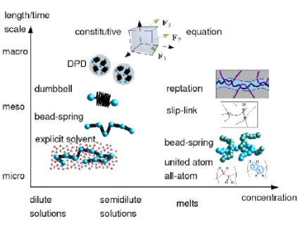
Figure 1: Different models of polymer dynamics are shown schematically for solutions and melts.

In general, examples of macroscopic constitutive equations employed to calculate polymer flow behavior include e.g. conformation tensor models like the Giesekus, Maxwell and FENE models but also the more recently proposed Pom-Pom, CCR and Rolie-Poly models birdwiest_review ; birdhco_review ; pompom ; wapperom_pompom ; likhtman_rolie ; marrucci_constitutive01 . For an overview, see Owens_computrheo ; Keunings_advances as well as the contributions by A.N. Beris and E. Mitsoulis in this volume. Most of these constitutive equations have been derived (or inspired) by simple mechanical models of polymer motion. They are mesoscale, kinetic theory models (based, e.g., on the dumbbell, FENE, bead-spring chain, and bead-rod chain analogues) capable of accounting for some important aspects of polymer dynamics, like chain stretching, non-affine deformation, diffusion, and hydrodynamic drag forces, either separately or all together pavlos_JOR1 . In polymer solutions, in particular, one should account for the solvent-mediated effect between beads (known as hydrodynamic interaction), which is usually modeled with the hydrodynamic resistance matrix DPL12 ; kimkarrila . Recently, an efficient simulation of solvent dynamics with the help of either the lattice Boltzmann saurobook ; duenweg_LBreview or the stochastic rotation dynamics SRD_colloidinshear ; SRD_review methods has been proposed with a suitable coupling of the bead dynamics. Besides their efficiency, these combined methods also incorporate non-uniformities and fluctuations in internal flow fields.

Usually, the mesoscopic, kinetic models are considered to be well-suited for predicting dynamical properties of polymer solutions on macroscopic scales. Details of the fast solvent dynamics are in most cases irrelevant for macroscopic properties. Exceptions are polyelectrolytes, where the motion of counterions in the solvent can have a major influence on polymer conformation. Therefore, more microscopic models of polyelectrolytes with explicit counterions are sometimes employed holm_PEreview (see also the contribution by M. Muthukumar in this volume). Another exception is the dynamics of individual biopolymers, e.g. protein folding, which is modeled with an all atomistic model including an explicit treatment of the (water) solvent molecules Shea_proteinfold .

For typical polymer melts, dumbbell models are inappropriate since they fail to account for the essential role of entanglements on the long-time dynamics. Successful mesoscopic, mean-field descriptions of entangled melts are offered by the reptation models doibook . Several modifications of the original Doi-Edwards-de Gennes reptation theory have been proposed in the last years in order to improve comparison to experiments in the linear and nonlinear flow regimes graham_tubeimproved ; likhtman_testtube ; marrucci_multimode ; hco117 ; hco119 ; hco123 ; hco129 ; meadlarsondoi . Recently, slip-link models have also been proposed jay_sliplink ; larson_sliplink ; jay_sliplink2 ; likhtman_sliplink ; doi_sliplink ; marrucci_sliplink ; marrucci_sliplink2 , providing a slightly more detailed description of entanglements, and which agree well with available experimental results.

At the microscopic level, polymer melts are modeled as multi-chain systems, see e.g. DPL12 ; mkbook ; Rigby_polymodels ; Kremer_ModelReview . For example, all-atom or united atom force fields, accounting explicitly for bond angle bending and torsion angle contributions (in addition to bond stretching and intermolecular interactions) Siepman ; Toxvaerd , are available. Different united-atom force fields are reviewed and compared e.g. in Rigby_polymodels ; Rousseau ; MatticeSuter . From such detailed atomistic molecular dynamics (MD) simulations, the linear viscoelastic properties can be computed by Green-Kubo relationships kubobook2 ; Barrat_Rouse ; Briels_CGreview . Also less detailed bead-spring models are available; a prototypical model is that of Kremer and Grest KremerGrest (or variants thereof loose ), which neglects chemical details and instead focuses on the interplay between chain connectivity and excluded volume effects. The non-linear regime can be studied by nonequilibrium molecular dynamics (NEMD) simulations, that directly address flow effect on polymer structure and conformation, both in shear and planar elongation (see e.g. mkbook ; loose ; todd_nemdreview ; toddreview ; mk_crossover ; brian_NEMD_1 ; brian_NEMD_2 ; chunggi_NEMD_1 ; chunggi_NEMD_2 and references therein). They are based on flow-adapted boundary conditions such as those proposed by Lees-Edwards for planar shear Lees_Edwards and by Kraynik-Reinelt for planar elongation Kraynik_Reinelt .

I.3 Challenges in standard simulations of polymers in flow

Despite the enormous advances in the field of molecular simulations Keunings_advances ; Binder_MCMDpoly ; Kremer_review03 ; Doros_simureview ; Doi_challenge ; Richter_dynsfac ; Cummings_NEMDandExp ; Tuzun_advancespolysimu , predicting the macroscopic flow properties of polymers from their underlying microstructure presents still major challenges Ober_polychallenge . Available MD and NEMD algorithms can address only time scales on the order of a few microseconds at most, implying that only short up to moderately entangled polymers can be studied in full atomistic detail in a brute-force manner. Extending the simulations to longer, truly entangled polymers is a first big task. Extending these flows to mixed or inhomogeneous flows is another big challenge. Among others, such a development would help understand the origin of interfacial slip and its mode (localized slip versus global slip) in the flow past a solid substrate. On the other hand, with the introduction of the revolutionary set of chain connectivity altering moves, extremely powerful Monte Carlo algorithms have been developed which have helped overcome the issue of the thermal equilibration of long polymers even at beyond equilibrium conditions vlasis_EB ; vlasis_Encyclopedia ; nikosPRL2002 ; Kremer_equilibrate ; Doros_CGreview . With the help of the end-bridging and double bridging moves, for example, truly long polyethylene (linear and branched) and polybutadiene systems have been equilibrated over the last years, which opened also the way to their topological analysis for the identification of entanglements martin_primitivepath ; Everaers_primitivepath ; Everaers_science ; Siheung ; hco142 ; hco145 ; brian_jnnfm .

Arguably the biggest challenge in polymer simulation under nonequilibrium conditions is to build well-founded multi-scale tools which can bridge the gap between microscopic information and macroscopically manifested viscoelastic properties, preferably through a constitutive equation founded on the microscopic model hco_lessons ; Doi_challenge . Simulations of metals face the same problem where again the objective is concurrent length scale simulations Tadmor_MRS ; Kaxiras_multiscalemetals ; to some extent, it is also relevant to simple fluids coveney_prl . For polymers, additional motivation stems from the increased interest in polymer mixtures and interfaces Milner_polyinterface resulting in morphology development at the nanoscale.

Here, we aim to shortly review some recent coarse-graining and multi-scale methods (see guenza_reviewCG ; Doros_CGreview ; Kremer_CGsimu08 ; Kremer_reviewMultiscale ; Briels_CGreview ; Kremer_multisimu ; plathe_CGinLNP ; Baschnagel_CGreview and also Nielaba_bridgingbook ; eijnden_progress ; Voth_CGbook ; Murtolo_MultiScaleSoftMatterreview for recent reviews of such methods for polymers and in a more general context, respectively), but also to put forward some new ideas for addressing such issues, which could eventually allow to model the macroscale quantities of interest by a suitable coarse-graining procedure. We will see that, if one is guided by nonequilibrium statistical mechanics and thermodynamics, it is possible to design well-founded multi-scale modeling tools that can link microscopic models with macroscopic constitutive equations. Such multi-scale modeling tools benefit from recently proposed approaches for static coarse graining which are mainly built on potentials of mean force Doros_CGreview ; Denton_reviewSoft ; Faller_CGreview . For dynamical properties, however, coarse-grained models need to account for dissipative effects that arise due to fast degrees of freedom that are eliminated (for example via projection operators) in favor of the remaining slowly varying ones Briels_CGreview ; alexander_workshop ; kubobook2 ; grabert . In a flow situation, these slow dynamical variables depart from their values in the quiescent fluid, while all other (faster) degrees of freedom track the evolution of the structural parameters; i.e., they are assumed to be in local equilibrium subject to the constraints imposed by the values of the structural parameters at all times. The proper definition of the set of the state variables, effectively representing the nonequilibrium states is the first key to the success of such an approach. Linking the microscopic model with a macroscopic model built on these slowly relaxing variables is the second key; as we will discuss in the next sections of this chapter, this is best addressed by getting guidance from a nonequilibrium statistical thermodynamics framework proposing a fundamental evolution equation for the macroscopic model in terms of the chosen structural (dynamical) variables.

II Coarse-grained variables and models

We start with a microscopic polymer model, whose state is specified by a point in $6N$–dimensional phase space, $\mathbf{z}\in\Gamma$ with $\mathbf{z}=(\mathbf{r}_{1},\ldots,\mathbf{r}_{N};\mathbf{p}_{1},\ldots,\mathbf{p}_{N})$ a short notation for the positions and momenta of all $N$ particles. The model is described by the microscopic Hamiltonian $H(\mathbf{z})$ with inter- and intra-molecular interactions. The coarse-grained model eliminates some of the (huge number of) microscopic degrees of freedom. The level of detail that is retained is specified by the choice of coarse-grained variables $\mathbf{x}=(x_{1},\ldots,x_{n_{\rm CG}})$ with

$$x_{k}=\langle\Pi_{k}\rangle\equiv\int_{\Gamma}\!{\rm d}\mathbf{z}\,\Pi_{k}(\mathbf{z})\rho(\mathbf{z}),\quad k=1,\ldots,n_{\rm CG},$$ (1)

where $\rho(\mathbf{z})$ denotes the probability distribution on $\Gamma$ and the phase space functions $\Pi_{k}(\mathbf{z})$ are the instantaneous values of the coarse-grained variables in the microstate $\mathbf{z}$.

Instead of the full, microscopic distribution $\rho(\mathbf{z})$, the coarse-grained model is already specified by the reduced probability distribution $p(\mathbf{x})\equiv\langle\delta(\mathbf{x}-\boldsymbol{\Pi}(\mathbf{z}))\rangle$. Knowledge of $p(\mathbf{x})$ allows to calculate averages of quantities $a(\boldsymbol{\Pi}(\mathbf{z}))$ via $\langle a(\boldsymbol{\Pi})\rangle=\int_{\Gamma}\!{\rm d}\mathbf{z}\,a(\boldsymbol{\Pi}(\mathbf{z}))\rho(\mathbf{z})=\int\!{\rm d}\mathbf{x}\,a(\mathbf{x})p(\mathbf{x})$. Instead of $p(\mathbf{x})$, coarse-grained models are often described by the so-called potentials of mean force $U_{\rm mf}(\mathbf{x})\equiv-k_{\rm B}T\ln p(\mathbf{x})$ which formally replace the Hamiltonian in the calculation of equilibrium, canonical averages. However, $U_{\rm mf}$ is an effective free energy difference and therefore depends on the thermodynamic state of the system. It contains in general effective many-body interactions that arise by partially integrating out microscopic degrees of freedom. For recent reviews see e.g. Denton_reviewSoft ; guenza_reviewCG ; kleinCGreview ; HansenLoewen_effPotreview .

Different sets of coarse-grained variables have been suggested in the literature and are briefly reviewed in the following. Usually, one is interested in a drastic reduction of microscopic complexity, so $n_{\rm CG}\ll 6N$. However sometimes, e.g. for equilibrating atomistic systems, a coarse-grained model with a modest reduction ($n_{\rm CG}$ only a factor 5 to 10 smaller than $6N$) might be useful. We emphasize that the mapping (1) as well as the corresponding probability $p(\mathbf{x})$ is not restricted to equilibrium situations. We proceed with a short review of coarse-grained variables and models that capture different levels of detail and briefly discuss their static and dynamic properties.

II.1 Beads and superatoms

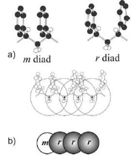
Figure 2: (a) Polystyrene $m$ and $r$ diads in transplanar conformation (for clarity, hydrogen atoms on phenyl rings have been omitted). (b) Illustration of a mapping scheme from the atomistic to a coarse-grained structure for PS wherein one bead corresponds to an $m$ or $r$ diad. [Reproduced with permission from plathe_reversevinyl , Figure 1.]

Coarse graining to the level of superatoms Faller_CGpolymer ; Faller_CGautomat ; Spyriouni ; Kamio ; plathe_effpotentials ; plathe_mapping ; plathe_mapvinyl ; plathe_reversevinyl ; Kremer_CGpolystyrene ; Kremer_CGpolystyrene06 ; KremerAbrams ; KremerLeo ; plathe_dendrimer ; pabloDNA ; Kremer_benzLC is a method followed when one wishes to reduce chemical complexity in a polymer chain without loosing the chemical identity of the molecule. According to this, a certain number of atoms or repeat units along the chain are grouped together into “superatoms” connected by effective bonds and governed by softer or smoother effective non-bonded interactions. The resulting (usually linear) chain sequence is simpler and amenable to fast thermal equilibration through application of state-of-the-art Monte Carlo algorithms slightly modified to account for the presence of the few different species along the chain. The method has been widely applied to reduce complexity and permit the molecular simulation of a number of polymers. Typical examples include polystyrene, poly(ethylene terepthalate), polycarbonates, polyphenylene dendrimers, even DNA. It involves computing the effective intra and intermolecular potentials among superatoms such that the coarse-grained model reproduces as faithfully as possible the structural, configurational and thermodynamic properties of the original atomistic polymer model. For vinyl chains presenting sequences of methylene (CH₂) and pseudo-asymmetric methyne (-CHR) groups along their backbone, the method should also account for the isotactic, syndiotactric or atactic stereochemistry of the polymer, based on the succession of meso ($m$) and racemo ($r$) diads (see Fig. 2).

According to Zwicker and Lovett Zwicker , if all interactions with potentials $V^{(n)}(\mathbf{r}_{1},\mathbf{r}_{2},\ldots,\mathbf{r}_{N})$, with $\mathbf{r}_{i}$ denoting the position vector of the $i$-th particle, in an $N$-atom molecular system consist of $n$-body and lower terms, then the system can be completely described by the knowledge of all $n$-order correlation functions $g^{(n)}(\mathbf{r}_{1},\mathbf{r}_{2},\ldots,\mathbf{r}_{N})$ and lower. Since, in practice, the complete determination of the $n$-point correlation functions is a huge task for $N\!>\!2$ and $n\!>\!4$, the calculations are usually limited to correlation functions that depend only on a single coordinate. For polymers where potential functions are usually separated into intra- and intermolecular ones, examples of such correlation functions include typically the radial distribution function, the distribution of bond lengths, the distribution of bending angles, and the distribution of dihedral angles. The coarse-grained potential then should be chosen such that it matches the distributions of all possible bond lengths, bond angles, and torsional angles, and of all intermolecular pair distribution functions, as extracted from simulations with the corresponding atomistic model.

For a distribution function that depends on a single coordinate, the corresponding effective potential can be computed through a method called iterative Boltzmann inversion method Faller_CGpolymer ; Spyriouni ; plathe_effpotentials ; Soper , aimed at matching the distribution of the relevant degrees of freedom (called target distribution) between the chosen coarse-grained model and the initial atomistic model for the polymer; the latter are usually extracted from accurate, brute-force MD simulations on short homologues. The method uses the differences in the potentials of mean force between the distribution function generated from a guessed potential and the true distribution function to improve the effective potential iteratively. Qualitative arguments for the conditions under which convergence should be expected have been discussed by Soper Soper .

Naive use of the coarse-grained potentials in standard molecular dynamics simulations leads to wrong predictions of diffusion and relaxation processes kleinCGreview ; plathe_CGwithDPD ; plathe_shearPS_CG . A simple, empirical method for relating the dynamics of superatoms at the coarse-grained level with the dynamics of true atomistic units at the atomic level uses a time rescaling factor depamaranas ; Kremer_DiffusRescaleTime . Within this method, the effective potentials are used in the reversible equations of motion of classical mechanics to perform standard molecular dynamics simulations and then an effort is made to match the mean-square displacements of the relevant structural units in the atomistic and coarse-grained models, both in amplitude and slope. Noid et al. Noid_CG1 ; Noid_CG2 formulate consistency criteria that should be obeyed when using coarse-grained potentials in equilibrium dynamical simulations.

Coarse graining to the level of superatoms has drawn a lot of attention in the last years mainly because of the capability to account for the correct stereochemical sequence of the repeat units. Despite the success of effective pair potentials in reproducing many of the structural properties of the corresponding atomistic system, however, their use in actual simulations is accompanied by a number of thermodynamic inconsistencies: (a) They perform well for the particular physical properties for which they were developed. For example, the value of pressure as computed by using the virial theorem from the effective potentials optimized with the iterative Boltzmann method is higher than what is observed in the atomistic system, unless an attractive perturbation potential is added (ramp correction to the pressure) and the potential is re-optimized. Given that in integral equation methods the mechanical properties of a system (such as pressure, energy and compressibility) are fixed by the singlet and pair number densities along with proper closures Zwicker ; Henderson_unique ; GrayGubbins , such a pressure inconsistency should be related to the degree of sensitivity of the site-site pair correlation function to the effective pair potential Soper . This is in line with the simulations of Jain et al. Jain_inverseMC who showed that, although there is a one-to-one correspondence between the structure of a liquid (i.e., the pair correlation function) and its pair-wise additive intermolecular potential (Henderson’s theorem Henderson_unique ), the convergence of potentials obtained by standard inversion procedures is extremely slow: although the repulsive part of the potential converges rapidly, its attractive part (to which, e.g., the internal energy and pressure are primarily sensitive) converges slowly. (b) Effective potentials are in general not transferable; they are state-point (e.g., temperature and pressure) dependent. In same cases, it has been noticed that temperature changes at about the same density do not drastically affect their parameterization plathe_transferCG ; Voth_CGdiffTemp . A newly developed effective force coarse-graining seems to improve transferability to other state points Voth_efforceCG . Developing fully self-consistent and transferable potentials at any arbitrary level of coarse graining remains still a challenge. (c) The coarse-grained system is considerably more compressible than the corresponding atomistic one. (d) Despite recent efforts, the proper use of coarse-grained potentials for dynamical simulations remains unclear. In particular the emergence of dissipation due to the coarse-graining step is mostly ignored, or, at best, included phenomenologically via some stochastic thermostat as done e.g. inGuerrault_DPDpoly ; plathe_CGwithDPD . For some notable exceptions see Briels_CGreview . Considerable work is definitely needed in order to arrive at a thermodynamically consistent description of a model system at the two levels of analysis (atomistic and coarse-grained), which will eliminate all these undesired symptoms and errors.

II.2 Uncrossable chains of blobs

Briels and collaborators BrielsPaddingtransient ; BrielsPaddinguncross ; Briels_CGchain ; Briels_CGdimer proposed a coarse-graining scheme wherein chains are sub-divided into a number of subchains of equal length; the center-of-mass of each such subchain is taken as the position of a corresponding mesoscopic particle called the blob. The blobs are connected by springs so that chain connectivity is preserved. Similarly to the coarse-graining procedure at the level of superatoms, the method makes use of a potential of mean force $U_{\rm mf}=V({\bf R}^{(n)})$ for the position vectors of the $n$ blobs, which ensures that the blob distributions in the atomistic and coarse-grained systems are the same.

In order to describe shear flow effects in a velocity field of the from $v_{x}(\mathbf{r})=\dot{\gamma}r_{y}$, Kindt and Briels BrielsPaddingtransient proposed making use of the SLLOD algorithm EvansMorriss_SLLOD . Starting with a Langevin equation, such a method results in the following expression for the blob dynamics:

$$M_{i}\frac{{\rm d}^{2}{\bf R}_{i}}{{\rm d}t^{2}} = {\bf F}_{i}^{S}-\zeta^{\rm eff}\left(\frac{{\rm d}{\bf R}_{i}}{{\rm d}t}-\dot{\gamma}P_{iy}\hat{\bf e}_{x}\right)+{\bf F}_{i}^{R}$$

$$\zeta^{\rm eff} = \zeta+\left[\sum_{i}({\bf F}_{i}^{S}\cdot{\bf P}_{i}-\dot{\gamma}P_{ix}P_{iy})\right]/\sum_{i}{\bf P}_{i}^{2}$$ (2)

where $\hat{\bf e}_{x}$ denotes the unit vector along the flow ($x$) direction, $M_{i}$ is the mass of the $i$-th blob particle, ${\bf R}_{i}$ its position vector, ${\bf F}_{i}^{S}=-\partial V/\partial{\bf R}_{i}$ the systematic force on particle $i$, $\zeta$ the friction coefficient, and ${\bf F}_{i}^{R}$ the random force on particle $i$. Since the coarse-grained bonded and nonbonded interactions are so soft that unphysical crossing of two bonds would not be prohibited, equations (II.2) are supplemented with an uncrossability constraint of the blob chains. Padding and Briels BrielsKindt ; BrielsPaddinguncross realized this constraint by a method which explicitly detects entanglements and prevents chain crossings through a geometric procedure. The procedure detects possible chain crossings and defines an entanglement point X at the prospective crossing site. Padding and Briels BrielsPaddingtransient ; BrielsPaddinguncross also proposed some non-trivial order-altering moves that lead to creation-removal of entanglements; these are important for the best possible realistic treatment of uncrossability constraints in simulations with the blob model. The Langevin equation of motion (II.2) contains the blob friction coefficient $\zeta$, whose calculation is not a straightforward issue even under equilibrium conditions. Despite this and its simplicity, the blob method has been found to capture correctly the viscoelastic properties of polymer melts with molecular length several times their entanglement length. From a numerical point of view, the method suffers from large requirements in CPU time, associated with the minimization algorithm for the location of entanglements which eventually limits simulations to chains made up of a finite number of blobs.

II.3 Primitive paths

A method to project atomistically detailed chains to smoother paths was proposed by Kröger et al. hco142 through a projection operation that maps a set $\{\mathbf{r}_{i}\}$, $i=1,2,\ldots,N$, of $N$ atomistic coordinates of a linear discrete chain to a new set $\{{\bf R}_{i}\}$ of $N$ coarse-grained ones defining a smoother path for the chain that avoids the kinks of the original chain but preserves somewhat its topology (the main chain contour). The projection involves only a single parameter, $\xi$, whose value was obtained by Öttinger hco155 by mapping the Porod-Kratky model (an atomistic model for a polymer chain) to a smoother chain with a Kuhn length equal to the entanglement length. In the limit of infinitely long chains, such a mapping suggests that the Kuhn length of the coarse-grained chain (the length of a segment between two entanglements) is equal to twice the tube diameter. The $\xi$-based method maps a particular chain onto a smoother path; however, the reduction of an ensemble of atomistic polymer chains to a mesh of primitive paths (PPs) as defined by the Doi-Edwards theory doibook requires that the projection satisfy not only chain continuity but also chain uncrossability. This subtle problem has been addressed only very recently through the seminal works of Everaers et al. Everaers_science , Kröger martin_primitivepath , and Tzoumanekas-Theodorou Doros_topos . Nevertheless, the simple $\xi$-based mapping has been very helpful in many respects; for example, it has allowed hco145 ; Tsolou to successfully calculate the zero shear rate viscosity of model polymer melts in the crossover regime from Rouse to entangled.

The topological analysis of Everaers et al. Everaers_science is based on the idea that PPs can be identified simultaneously for all polymer molecules in a bulk system by: keeping chain ends fixed in space, disabling intra-chain excluded-volume interactions and retaining the inter-chain ones, and minimizing the energy of the system by slowly cooling down toward the zero Kelvin temperature. This causes bond springs to reduce their length to zero, pulls chains taut, and results in a mesh of PPs consisting of straight segments of strongly fluctuating length and more or less sharp turns at the entanglement points. The method can be modified Everaers_primitivepath ; Kremer_entangled05 ; Uchida_actin to preserve self-entanglements or to distinguish between local self-knots and entanglements between different sections of the same chain.

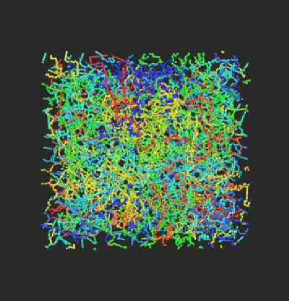
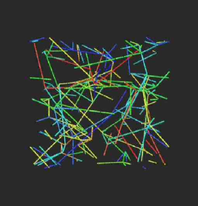
Figure 3: (a) A snapshot of a fully equilibrated atomistic configuration of a 40-chain C₅₀₀ trans-1,4-PB melt at 500K and 1atm. (b) The corresponding entanglement network mesh as computed with Kröger’s method martin_primitivepath .

Kröger martin_primitivepath also presented an algorithm which returns a shortest path and the related number of entanglements for a given configuration of a polymeric system in 2-D and 3-D space, based on geometric operations designed to minimize the contour length of the multiple disconnected path (i.e., the contour length summed over all individual PPs) simultaneously for all chains in the simulation cell. The number of entanglements is simply obtained from the shortest path as either the number of interior kinks, or from the average length of a line segment. Application of the algorithm to united-atom models of linear polyethylene (PE) foteinopoulou allowed the calculation of a number of important statistical properties characterizing its PP network at equilibrium and helped make the connection with an analytic expression for the PP length of entangled polymers by Khaliullin and Schieber jay_pathlength following earlier works DoiKuzuu ; shanbaglarson . A representative snapshot of the entanglement network as computed for a linear trans-1,4-PB polymer (40 chains of C₅₀₀ at $T$=450K and $P$=1atm) with Kröger’s method is shown in Fig. 3.

A third methodology for reducing chains to shortest paths has been presented by Tzoumanekas and Theodorou Doros_topos where topological (chain uncrossability) constraints are defined as the nodes of an entanglement network. Through their contour reduction topological analysis (CReTA) algorithm, an atomistic configuration of a model polymer sample is reduced to a network of corresponding PPs defined by a set of rectilinear segments (entanglement strands) coming together at nodal points (entanglements) by implementing random aligning string moves to polymer chains and hard core interactions. In addition to obtaining topological measures for a number of entangled polymers, Tzoumanekas and Theodorou Doros_topos found that data for the normalized distribution of the reduced number of monomers (united-atoms or beads) in an entanglement strand are well described by a master curve suggesting a universal character for linear polymers. As analyzed by Tzoumanekas-Theodorou Doros_topos , the master curve is also obtainable in terms of a renewal process generating entanglement events stochastically along the chain.

Apart from some algorithmic details, the three methods lead to practically similar conclusions as far as the topological state of many entangled linear polymer melts (PE, PB, PET and PS) is concerned. A significant result of all of them (see, e.g., Doros_topos ) is that the ensemble average of the number of monomers per entanglement strand $\bar{N}_{\rm ES}$ as computed directly from the topological analysis is significantly smaller than the corresponding quantity $N_{\rm e}$ measured indirectly through $N_{\rm e}=N\langle{R^{2}}\rangle/\langle L\rangle^{2}$ by assuming that PP conformations are random walks. This is due to directional correlations between entanglement strands along the same PP, which decay exponentially with entanglement strand separation. Therefore PPs are not random walks at the length scale of the network mesh size.

II.4 Other single-chain simulation approaches to polymer melts: slip-link and dual slip-link models

Doi and Edwards DoiEdwards78 and Doi and Takimoto DoiTakimoto have proposed a description of an entangled polymer in terms of a slip-link model that can cumulatively account for chain confinement and constraint release in a consistent way. Slip-links do not represent an entanglement junction in real space; they are rather virtual links representing effective constraints whose statistical character is determined by other polymers. In the dual slip-link version of the model, the slip-link confines a pair of chains (and not a single chain). Masubuchi and collaborators marrucci_sliplink ; marrucci_sliplink2 ; Marrucci_tubedilate ; Marrucci_comparesliplink generalized the idea by regarding a slip-link as an actual link in real space. In their formulation, each polymer chain is represented as a linear sequence of entanglement strands considered as segments (phantom entropic springs) joining consecutive entanglement points (the beads) along the chain. These Rouse-like chains are all inter-connected by slip-links at the entanglement points to form a 3-D primitive chain network. The system is described by: the number $Z$ of segments in each chain, the number $n$ of monomers in each chain segment, and the position vectors ${\bf R}_{i}$ of the slip-links or entanglement points. These state variables are postulated to obey certain Langevin-type governing equations in which the single relevant parameter of the primitive chain network is the average value $\langle Z\rangle$ of entanglements per chain. Defining the model functions and parameters on the basis of the results obtained from one of the three topological analysis discussed above leads to rheological predictions that follow quite satisfactorily experimental data for many polymer melts in shear but deviations are observed when the model is used to describe the elongational rheology of these systems. A generalization of the slip-link idea by Schieber and collaborators jay_sliplink ; jay_sliplink2 to a full-chain slip-link model with a mean-field implementation of constraint release and constant chain friction (as opposed to constant entanglement friction) has been shown to provide accurate predictions of the $G^{\prime}$ and $G^{\prime\prime}$ spectra for many polymer melts (such as PS, PB and PIB).

II.5 Entire molecules

In dilute polymer solutions, coarse graining polymer coil or star polymers to a a system of interacting soft particles has been explored in Louis_CGpolymsoft ; Louis00 ; Louis01 . Kindt and Briels Briels_CGnij ; BrielsKindt proposed such a type of coarse graining also for polymer melts where an entire chain is represented as a single particle. To account for the presence of entanglements which are considered to be responsible for the distinct viscoelastic properties exhibited by polymers, Kindt and Briels Briels_CGnij ; BrielsKindt introduced a second set of variables, the number $n_{ij}$ of entanglements between chains $i$ and $j$. This governs the degree of interpenetration or overlapping of two chains whose centers-of-mass are fixed at a given distance. The state of the system is thus fully determined by the position vectors ${\bf R}_{i}$ of the centers-of-mass of the $N_{\rm ch}$ chains and the $N_{\rm en}=N_{\rm ch}(N_{\rm ch}-1)/2$ entanglement numbers $n_{ij}$. The equilibrium density distribution function $\Psi$ for such a system is of the form:

$$\Psi\left({\bf R}^{(N_{\rm ch})},n^{(N_{\rm en})}\right)\sim\exp\left\{{-\frac{1}{k_{\rm B}T}\left[{U_{\rm mf}({\bf R}^{(N_{\rm ch})})+{\sum_{i,j}{\frac{1}{2}\alpha\left({n_{ij}-n_{0}(r_{ij})}\right)^{2}}}}\right]}\right\}$$ (3)

where $k_{\rm B}$ is Boltzmann’s constant, $T$ the temperature, $U_{\rm mf}$ the potential of mean force, the double summation is over all interacting particle pairs, and $\alpha$ is a constant determining the strength of the fluctuations around a mean number $n_{0}(r_{ij})$ of entanglements between chains $i$ and $j$. $n_{0}(r_{ij})$ is like an order parameter governing the “friction” felt by each chain and generating restoring elastic forces. According to Eq. (3), integration over $n_{ij}$ results in a Boltzmann distribution for the $N_{\rm ch}$ coordinates ${\bf R}_{i}$, thus the equilibrium statistics of the system is not altered by the introduction of the entanglements. Typical expressions for $U_{\rm mf}$ have been discussed by Padding and Briels BrielsPaddingtransient ; BrielsPaddinguncross but also by Pagonabarraga and Frenkel Frenkel_DPD2000 ; Frenkel_DPD2001 in their derivation of the “multi-particle dissipative particle dynamics” method. The method is capable of providing structural information only about the radial distribution function $g(r)$ of the centers-of-mass of the chains. Representative results for a number of linear PE melts revealed a small correlation hole effect at the level of entire chains, which is consistent with data reported by Mavrantzas-Theodorou vlasis_freeenergyelong through atomistic Monte Carlo simulations. No other signals of local structure could be discerned. Clearly, accounting for entanglements (which is necessary in order to produce the correct viscoelastic properties) seems to have a negligible effect on the structural properties at the level of entire chains.

The single particle model has been proposed to describe systems where memory effects are dominant. This is the case for example of complex fluids involving colloidal particles floating in a solvent in which a small amount of polymer is also dissolved. In this model, dynamics is described Briels_CGnij ; Briels_CGslow by generating (according to standard expressions for Smoluchowski-type equations) at every time step ${\rm d}t$ not only a displacement ${\rm d}{\bf R}_{i}$ in the position of each particle $i$ but also a change ${\rm d}n_{ij}$ in the number of entanglements. Memory effects are taken into account through transient forces: when two particles come together such that temporarily $n_{ij}<n_{0}$, their coronas are pushed apart causing a repulsion between the two particles. On the other hand, if the coronas are separated enough such that temporarily $n_{ij}>n_{0}$, the particles experience attractive forces. These phenomena cannot be studied by traditional Brownian Dynamics simulations where delta-correlated random displacements are assumed. Figure 4 shows the viscosity obtained from such a method referring to a typical resin with particles having a hard core diameter of 100 nm. The very same model has been successful in describing also shear banding and the chaining of dissolved colloids in viscoelastic systems Briels_CGcoreshell .

II.6 Conformation tensor

Based on the idea that, in a flow situation, certain structural variables depart from their values in the quiescent fluid while all other (faster) degrees of freedom are at equilibrium subject to the constraints imposed by the values of the slow variables at all times, coarse-grained models have also been developed where chains are described at the level of the conformation tensor $\mathbf{c}$ DPL12 ; mkbook ; birdwiest_review ; vlasis_elong ; Rutledge_QQ . The latter might be defined via the average gyration tensor or via the tensorial product of the end-to-end vectors. The choice of $\mathbf{c}$ among the structural parameters marks a description in terms of a tensorial variable. In addition to a single conformation tensor one can envision a description in terms of many (higher-mode) conformation tensors, corresponding to the Rouse or bead-spring chain model. In general vlasis_elong , from an $N$-mer chain, $N(N-1)/2$ different conformation tensors $\mathbf{c}_{ij}$, $i,j=1,2,\ldots,N-1$ can be constructed, each one being identified as a properly dimensionalized average dyadic $\left\langle{\mathbf{Q}_{i}\mathbf{Q}_{j}}\right\rangle$ with $\mathbf{Q}_{i}$ denoting the connector vector between mers $i+1$ and $i$ along the chain DPL12 .

For systems of entangled polymer chains, reptation theory suggests the distribution function of primitive path orientations as structural variable, see previous section. If chains contain long chain branches that can significantly affect the rheological response of the system, their contribution to overall system dynamics should also be accounted. This is the case, for example with H-shaped polymers for which a model built on two structural parameters, the tube orientation tensor S from one branch to the other branch along the chain, and a scalar quantity $\Lambda$ describing the length of the tube divided by the backbone tube length at equilibrium, has been proposed pompom ; hco_pompom . This marks a description at the level of a tensorial and a scalar.

The description in terms of a few, well-defined structural parameters (such as the conformation tensor, the configurational probability function, and the orientation tensor and a scalar) is very appealing because of the existence of well-founded models developed under the GENERIC framework of non-equilibrium thermodynamics hcogenbook . In Section IV, we will see that, among other things, this allows building thermodynamically guided multi-scale approaches by expanding the equilibrium statistical ensemble to incorporate terms involving conjugate variable(s) driving the corresponding structural parameters away from equilibrium. The GENERIC formalism here is an extremely useful tool, since it can guide us in linking the conjugate variable(s) to the applied flow field. It is not surprising therefore that this class of coarse-graining procedures constitutes one of the most understood and best-founded today.

II.7 Mesoscopic fluid volumes

For the numerical simulation of flowing polymers, several mesoscopic models have been proposed in the last years that describe polymer (hydro-)dynamics on a mesoscopic scale of several micrometers, typically. Among these methods, we like to mention Dissipative Particle Dynamics (DPD) DPD1992 , Stochastic Rotation Dynamics (sometimes also called multiparticle collision dynamics) SRD_review , and Lattice Boltzmann algorithms saurobook . Hybrid simulation schemes for polymer solutions have been developed recently, combining these methods for solvent dynamics with standard particle simulations of polymer beads (see e.g. SRD_colloidinshear ; kaxiras_DNAtranslocation ; winkler_MPC04 ). Extending the mesoscopic fluid models to non-ideal fluids including polymer melts is currently in progress Frenkel_DPD2000 ; Frenkel_DPD2001 ; Ihle_nonidealMPC ; saurobook .

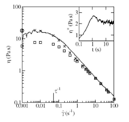
Figure 4: Viscosity versus shear rate for a typical resin, as obtained from the particle model of Kindt and Briels Briels_CGnij and van der Noort et al. Briels_CGslow . The solid line represents experimental data while the crosses are simulation results including all forces in the stress tensor. The squares represent viscosities based on the conservative forces only. The circle at the vertical axis gives the zero-shear viscosity according to the Green-Kubo formula. In the inset, we show the overshoot in the instantaneous value of the viscosity at $\dot{\gamma}=$1s^-1. [Reproduced with permission from Briels_CGslow , Figure 3.]

III Systematic and thermodynamically consistent approach to coarse graining: general formulation

III.1 The need for and benefits of consistent coarse-graining schemes

Under equilibrium conditions, statistical thermodynamics forms a bridge between thermodynamics (whose goal is the understanding and prediction of macroscopic phenomena) and molecular physics (which focuses on the intermolecular interactions between the atoms making up the system). It provides therefore an interpretation of thermodynamic quantities from a molecular point of view. For a number of complex fluids (like colloids, liquid crystals, and polymers), information at a mesoscopic level of description (intermediate to molecular and macroscopic ones) is often extremely useful in understanding and predicting material behavior (see e.g. Sect. II and mkbook ). At equilibrium, statistical thermodynamics provides the framework for understanding system properties also at these intermediate scales. For example, as mentioned in Sect. II.1, effective potentials describing interactions between coarse-grained (pseudo-)particles can systematically be derived by integrating out irrelevant degrees of freedom.

Although extensions to capture dynamics at a mesoscopic level are in progress (see Sect. II), most descriptions in terms of coarse-grained particles are so far largely restricted to equilibrium situations. For example, the recently proposed time rescaling approach (see Kremer_CGpolystyrene ; Kremer_DiffusRescaleTime ) for coarse-grained models does not seem appropriate to fully account for the increase in dissipation inherent in any meaningful coarse graining technique. We mention the case of hydrodynamic interactions in polymer solution which necessitate a description not in terms of a scalar frictional variable but in terms of a tensorial friction matrix.

Dissipation and friction are more properly accounted for in Briels_CGreview ; BrielsPaddingtransient ; BrielsPadding ; Briels_CGdimer ; Briels_CGchain . These authors, however, arrive at a daunting assessment: “We therefore conclude that coarse-grained models lack thermodynamic consistency” Briels_CGchain . As we will demonstrate below, for appropriately defined coarse-grained models, there is a way to restore thermodynamic consistency. So, contrary to the authors of Briels_CGchain , we believe that the recently introduced GENERIC formalism of nonequilibrium thermodynamics offers a framework for the development of true and complete coarse-graining strategies hco_lessons , in the sense that: (a) the resulting model is well-behaved and thermodynamically consistent, (b) it can be parameterized based on the information provided by a lower resolution model, and (c) it can be improved based on microscopic simulations targeted to address the relevant structural variables and their dynamic evolution. Of course, a word of caution is in place here: coarse-grained models based on the GENERIC framework will rely on a number of strong assumptions (inherent to most projection operator based methods) implying a description in terms of a set of carefully chosen slowly-evolving state variables. The underlying assumption behind such a description is that of the existence of a clear time-scale separation between the evolution of these (slow) variables and that of the (eliminated) fast or irrelevant ones. The coarse-grained model of Briels_CGchain , for example, involves lumping ten beads along a chain into one or two blobs, for which the time-scale separation argument is questionable. Their negative conclusion about the thermodynamic consistency of the model is therefore not surprising.

III.2 Different levels of description and the choice of relevant variables

Coarse-graining connects (at least) two descriptions of the same system at two different levels of detail: a low-resolution level and a higher-resolution level. We focus attention here to the case where the high-resolution level is the atomistic one, although this is not necessary hco_projectors .

We consider a point in phase space $\mathbf{z}\in\Gamma$, where $\mathbf{z}=(\mathbf{r}_{1},\ldots,\mathbf{r}_{N};\mathbf{p}_{1},\ldots,\mathbf{p}_{N})$ is a short hand notation for the positions $\mathbf{r}_{i}$ and momenta $\mathbf{p}_{i}$ of all $N$ particles, at the microscopic level; this, for example, could be an all-atom or a united atom model or even the simpler and computationally more convenient FENE bead-spring model mkbook . All these three models are classified here as microscopic models due to the absence of dissipation and irreversibility. Dynamics at the microscopic model is governed by Hamilton’s equation of motion

$$\dot{\mathbf{z}}={\bf J}\cdot\frac{\partial H}{\partial\mathbf{z}}$$ (4)

where $H(\mathbf{z})$ is the microscopic Hamiltonian and ${\bf J}$ the symplectic matrix. Equivalently, Hamilton dynamics can be formulated by $\dot{A}=\{A,H\}$, where $\{A,B\}$ denotes the microscopic Poisson bracket between arbitrary functions $A(\mathbf{z})$ and $B(\mathbf{z})$. We recall that the basic properties of Poisson brackets are their anti-symmetry $\{A,B\}=-\{B,A\}$, the Leibniz rule $\{AB,C\}=A\{B,C\}+\{A,C\}B$, and the Jacobi-identity, $\{A,\{B,C\}\}+\{B,\{C,A\}\}+\{C,\{A,B\}\}=0$ hcogenbook .

Due to their very long relaxation times, there is a clear gap between the time scales that can be addressed in microscopic simulations of polymer melts and the relevant time scales in experimental studies. Although this prevents the direct applicability of brute-force microscopic simulations, it renders them ideal systems for a comprehensive understanding over multiple time and length scales by embodying the concept of multiscale modeling. The first and more important step in this context is the proper choice of the relevant variables at the coarser level. For simple fluids, densities of conserved quantities (mass, momentum, and energy) are the proper variables to consider if one is interested in hydrodynamic properties. For systems with broken symmetries, the corresponding order parameters constitute additional candidates for slow variables ChaikinLubensky . In the case of complex fluids, however, no general rules are available how the appropriate relevant variables should be chosen, and this emphasizes the importance of physical intuition kubobook2 ; grabert for the choice of variables beyond equilibrium.

For polymers, one can be guided by available theoretical models. For example, orientational ordering in liquid crystals and liquid crystalline polymers can be described by the alignment tensor within the Landau-de Gennes theory doibook . Birefringence and viscous properties in the case of unentangled polymer melts can be addressed by models based on the concept of a conformation tensor, see Sect. II.6. For branched polymers, a scalar variable is added to the conformation tensor in order to capture additional contributions to the stress tensor pompom due to long arm relaxations. For entangled polymer melts, reptation theory provides a description in terms of a probability distribution function for the orientation of segments along the primitive path DPL12 ; doibook .

These theories are examples of mesoscopic or macroscopic models that lead to closed-form constitutive equations. Furthermore, they can all be described in the context of the single-generator bracket berisbook or the GENERIC hcogenbook formalisms of nonequilibrium thermodynamics,

$$\dot{\mathbf{x}}={\bf L}\cdot\frac{\delta E}{\delta\mathbf{x}}+{\bf M}\cdot\frac{\delta S}{\delta\mathbf{x}}.$$ (5)

In (5), $E(\mathbf{x})$ and $S(\mathbf{x})$ are the coarse-grained energy and entropy functions, respectively. The anti-symmetric operator ${\bf L}$ defines a generalized Poisson bracket $\{A,B\}=\frac{\delta A}{\delta\mathbf{x}}\cdot{\bf L}\cdot\frac{\delta B}{\delta\mathbf{x}}$ which shares the same properties as the classical Poisson bracket described above. The last term in (5) is new compared to Hamiltonian dynamics (4) and describes dissipative, irreversible phenomena. The friction matrix ${\bf M}$ is symmetric and positive, semi-definite. Together with the degeneracy requirements ${\bf L}\cdot(\delta S/\delta\mathbf{x})={\bf M}\cdot(\delta E/\delta\mathbf{x})=0$, these properties ensure that the total energy $E$ is preserved and $S$ is not decreasing in time hcogenbook .

The mesoscopic and macroscopic models come with a number of parameters, e.g.  mean-field potentials, friction coefficients, effective relaxation times, etc., whose connection to molecular terms is not straightforward. It is the purpose of thermodynamically-guided, systematic coarse graining methods to address this issue.

III.3 GENERIC framework of coarse graining

Coarse graining implies a description in terms of a few, carefully chosen variables after the elimination of all irrelevant degrees of freedom. Inevitably, this comes together with entropy generation (irreversibility) and dissipation. In the GENERIC formalism hco_projectors ; hcogenbook , the emphasis is then shifted from the fundamental time evolution equation itself to the individual building blocks of that theory (5), and opens up the way toward the development of consistent coarse-graining strategies. The interested reader is referred here to Ref. hco_lessons . More details on the statistical mechanics of coarse graining can be found in kubobook2 ; hcogenbook ; Pep_CGStatMech ; for coarse graining of simple fluids within the GENERIC framework, see hco_simplefluid ; henning10 .

III.3.1 Mapping to relevant variables and reversible dynamics

For every microstate $\mathbf{z}$ of the system, the instantaneous values of the relevant variables are defined by a set of phase space functions $\boldsymbol{\Pi}(\mathbf{z})$. The functions $\boldsymbol{\Pi}(\mathbf{z})$ cannot generally be identified with $\mathbf{x}$; they are rather connected with $\mathbf{x}$ through $\mathbf{x}=\langle\boldsymbol{\Pi}(\mathbf{z})\rangle$, i.e., as averages based on a suitable probability density $\rho_{\mathbf{x}}(\mathbf{z})$ at the microscopic phase space $\Gamma$. Thus, the coarse-grained energy $E(\mathbf{x})$ is obtained from the microscopic Hamiltonian $H(\mathbf{z})$ by straightforward averaging,

$$E(\mathbf{x})=\langle H(\mathbf{z})\rangle_{x},$$ (6)

and, similarly, the coarse-grained Poisson bracket is obtained from the average of the classical Poisson bracket,

$$\{A,B\}=\frac{\delta A}{\delta x_{k}}L_{kl}\cdot\frac{\delta B}{\delta x_{l}};\quad L_{kl}(\mathbf{x})=\langle\{\Pi_{k},\Pi_{l}\}\rangle_{x}.$$ (7)

Eqs. (6) and (7) define the reversible part of GENERIC (5) in terms of a coarse-grained Poisson bracket dzyalo ; ChaikinLubensky . The additional terms related to dissipation and increase in entropy have to be accounted for by the irreversible contribution to GENERIC (5) and are described just below.

III.3.2 Irreversibility and dissipation through coarse graining

The fact that we do not account explicitly for the irrelevant variables at the level of the GENERIC framework leads to entropy increase and additional dissipation at the coarser level of description hco_lessons .

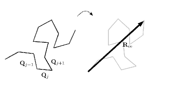
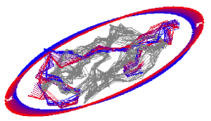
Figure 5: (a) Schematic illustration of freely jointed chain with end-to-end vector $\mathbf{R}_{\rm ee}$. (b) Fluctuations of polymer chain in shear flow around stationary state. Ellipses indicate the eigenvalues and orientation of eigenvector of $\langle\mathbf{R}_{\rm ee}\mathbf{R}_{\rm ee}\rangle$. [Figure courtesy of M. Kröger, ETH Zürich.]

To illustrate this, let us consider the simple example of a freely jointed chain, shown schematically in Fig. 5a. We can describe such a chain by the set of all connector vectors ${\bf Q}_{j}\equiv\mathbf{r}_{j+1}-\mathbf{r}_{j}$, $j=1,\ldots,N$. All admissible configurations with $|{\bf Q}_{j}|=b$ have equal probability. If we decide choose the end-to-end vector $\mathbf{R}_{\rm ee}$ as the only relevant variable, then there are in general many configurations $\{{\bf Q}_{j}\}$ which are compatible with $\mathbf{R}_{\rm ee}$. The coarse-grained entropy $S(\mathbf{R}_{\rm ee})$ is a measure of the number of these configurations. One finds that the probability of $\mathbf{R}_{\rm ee}$ is Gaussian around $\mathbf{R}_{\rm ee}=0$, which implies that there are many more coiled configurations compared to stretched ones. The associated entropy $S(\mathbf{R}_{\rm ee})=S(0)-3\mathbf{R}_{\rm ee}^{2}/2Nb^{2}$ decreases for chains undergoing stretching and leads to a restoring force which is known as “entropic spring” in coarse-grained polymer models DPL12 . This illustrates the emergence of (additional) entropy through coarse graining.

We turn now to the discussion of the probability distribution $\rho_{\mathbf{x}}(\mathbf{z})$. In sharp contrast to equilibrium statistical mechanics, there are unfortunately no general results for the probability distribution of nonequilibrium states. Even for nonequilibrium stationary states there are at present only a few results for very special model systems available (see e.g. Zia_NESSclass ). Systems, however, where the time-scale separation assumption holds are well described within the quasi-equilibrium approximation that treats the nonequilibrium system as an equilibrium one for the present values of relevant variables Jaynes57 ; zubarevbook ; karlinbook . In the generalized microcanonical ensemble, all microstates $\mathbf{z}$ that are compatible with given values of the relevant variables $\Pi(\mathbf{z})$ have equal probability. The corresponding entropy is a measure of the number of such microstates $\mathbf{z}$ that are compatible with a given coarse-grained state. For practical calculations, it is more convenient to pass to the generalized canonical distribution. In analogy to equilibrium statistical mechanics, the average values $x_{k}=\langle\Pi_{k}(\mathbf{z})\rangle_{x}$ are constrained to prescribed values with the help of Lagrange multipliers $\Lambda_{k}$. The generalized canonical distribution can then be obtained from the maximum entropy principle and reads

$$\rho_{\mathbf{x}}(\mathbf{z})=\frac{e^{-\sum_{k}\Lambda_{k}\Pi_{k}(\mathbf{z})}}{\int_{\Gamma}\!{\rm d}\mathbf{z}\,e^{-\sum_{l}\Lambda_{l}\Pi_{l}(\mathbf{z})}}$$ (8)

where the $\Lambda_{k}$’s have to be chosen so as to satisfy $x_{k}=\int\!{\rm d}\mathbf{z}\,\Pi_{k}(\mathbf{z})\rho_{\mathbf{x}}(\mathbf{z})$. The quasi-equilibrium entropy associated with Eq. (8) is

$$S(\mathbf{x})=k_{\rm B}\sum_{k}\Lambda_{k}x_{k}+k_{\rm B}\ln\int_{\Gamma}\!{\rm d}\mathbf{z}\,e^{-\sum_{l}\Lambda_{l}\Pi_{l}(\mathbf{z})}.$$ (9)

The coarse-grained entropy plays the role of an effective potential for the relevant variables. Determining the functional form of $S(\mathbf{x})$ from (9) presents a challenge, since the explicit expression for the Lagrange multipliers $\Lambda_{k}(\mathbf{x})$ is in general unknown. A successful method for extracting at least partial information on $S(\mathbf{x})$ has been explored in vlasis_elong from atomistic simulations of a polymer melt in elongational flow. We discuss this issue further in Sects. IV.2 and IV.3.

Having specified the nonequilibrium ensemble and coarse-grained entropy, we finally like to discuss the increase of dissipation through coarse graining in more general terms. We have seen above that many microstates (values of connector vectors) are in general compatible with a given coarse-grained state (defined by the value of the end-to-end vector in the above example). Conversely, this implies that a coarse-grained state does not uniquely determine the microstate. The dynamics on the coarse-grained level has necessarily a stochastic character which is known as fluctuations, see Fig. 5b. If those fluctuations are correlated in time, they have to be accompanied by dissipation, as required by the fluctuation-dissipation theorem kubobook2 . These qualitative observations are put into a solid theoretical framework by the projection operator formalism grabert . It should be emphasized that projection operators provide exact relations for any set of variables in terms of complicated integro-differential equations. Simpler, closed-form equations without a memory integral, however, result only in cases when the time-scale of the chosen variables is well-separated from those of the irrelevant ones grabert ; Pep_harmonicMarkov . A prominent example where this assumption seems not to be met is the dynamics of glassy polymers, where usually mode-coupling approximations for the memory kernel are employed Schweizer_MCTpolymer ; Fuchs_MCTpolymer . We here insist on the time-scale separation, which severely restricts possible choices of relevant variables where such a separation can hold. For glassy polymers and glasses, in general, an appropriate set of relevant variables is not known at present, although some promising first steps have been taken recently hco_glass ; ema_nonaffine . These restrictions are the price to pay for a proper coarse-grained description with a well-defined entropy and without accounting for memory effects. In this case, the dissipation matrix ${\bf M}$ as derived from the projection operator formalism reads

$$M_{kl}=\frac{1}{k_{\rm B}}\int_{0}^{\tau_{s}}\!{\rm d}t\,\langle\dot{\Pi}_{k}^{\rm f}(t)\dot{\Pi}_{l}^{\rm f}(0)\rangle,$$ (10)

where $\dot{\Pi}_{k}^{\rm f}$ is the fast part of the time derivative of the macroscopic variables hco_projectors ; zubarevbook ; hcogenbook . The separating time scale $\tau_{s}$ should be chosen large enough to comprise all the fast fluctuations that are not captured on the coarse-grained level hcogenbook . Thus, the friction matrix ${\bf M}$ arises due to fast fluctuations that are not resolved at the coarser level. The numerical evaluation of the dissipation matrix (10) for a polymer melt is described in Sect. IV.3.

IV Thermodynamically guided coarse-grained polymer simulations beyond equilibrium

IV.1 GENERIC coarse-graining applied to unentangled melts: foundations

Unentangled polymer melts are usually described in terms of the conformation tensor which provides an overall picture of the entire polymer chain. From the point of view of the GENERIC formalism, this implies a description where, in addition to the hydrodynamic fields mass $\rho$, momentum $\mathbf{g}$, and energy density $\epsilon$, the conformation tensor $\mathbf{c}$ is also included in the vector of state variables,

$$\mathbf{x}=(\rho,\mathbf{g},\epsilon,\mathbf{c}).$$ (11)

Let $\mathbf{z}=(\mathbf{r}_{1},\ldots,\mathbf{r}_{N};\mathbf{p}_{1},\ldots,\mathbf{p}_{N})$ denote the microstate defined by the positions and momenta of all particles. The chosen macroscopic variables $\mathbf{x}=\langle\boldsymbol{\Pi}(\mathbf{z})\rangle$ are defined as follows. The mass density is defined by

$$\rho(\mathbf{r};t)=\langle\sum_{j}m_{j}\delta(\mathbf{r}-\mathbf{r}_{j}(t))\rangle\equiv\langle\Pi_{\rho}\rangle,$$ (12)

where $m_{j}$ denotes the mass of particle $j$. Similarly, the momentum density is obtained by

$$\mathbf{g}(\mathbf{r};t)=\langle\sum_{j}\mathbf{p}_{j}\delta(\mathbf{r}-\mathbf{r}_{j}(t))\rangle\equiv\langle\boldsymbol{\Pi}_{g}\rangle.$$ (13)

From $\rho$ and $\mathbf{g}$, the macroscopic velocity field $\mathbf{v}(\mathbf{r})$ is defined by $\mathbf{v}(\mathbf{r})=\mathbf{g}(\mathbf{r})/\rho(\mathbf{r})$. The total energy density can be expressed as

$$\epsilon(\mathbf{r};t) = \langle\sum_{j}\hat{e}_{j}\delta(\mathbf{r}-\mathbf{r}_{j}(t))\rangle\equiv\langle\Pi_{\epsilon}\rangle,$$ (14)

where $\hat{e}_{j}=(1/2)m_{j}\mathbf{u}_{j}^{2}+\Phi_{j}$ with $\mathbf{u}_{j}=\mathbf{p}_{j}/m_{j}-{\bf v}(\mathbf{r}_{j})$ the peculiar velocity of particle $j$ and $\Phi_{j}$ the potential energy of particle $j$. Finally, the additional, internal variable $\mathbf{c}$ is a symmetric, second-rank tensor which is defined by

$$\mathbf{c}(\mathbf{r};t)=\frac{1}{N_{\rm ch}}\sum_{a=1}^{N_{\rm ch}}\langle\hat{\boldsymbol{\Pi}}^{a}\delta(\mathbf{r}-\mathbf{r}_{c}^{a}(t))\rangle\equiv\langle\boldsymbol{\Pi}_{c}\rangle,$$ (15)

where $N_{\rm ch}$ is the number of chains in the system and $N_{a}=\sum_{j\in I_{a}}$ the number of particles in chain $a$. The center of mass of polymer $a$ is denoted by $\mathbf{r}_{c}^{a}=N_{a}^{-1}\sum_{j\in I_{a}}\mathbf{r}_{j}$. The tensor $\hat{\boldsymbol{\Pi}}^{a}$ is a conformation tensor of a single chain and quantifies the instantaneous, internal structure of polymer $a$. Examples are the gyration tensor $\hat{\boldsymbol{\Pi}}^{a}=N_{a}^{-1}\sum_{j\in I_{a}}(\mathbf{r}_{j}-\mathbf{r}_{c}^{a})(\mathbf{r}_{j}-\mathbf{r}_{c}^{a})$ or the tensor product formed either by the end-to-end vector or the first Rouse mode.

The macroscopic energy $E$ is obtained by straightforward averaging of the microscopic Hamiltonian, see Eq. (6).

The resulting expression for the distribution function of the generalized canonical ensemble reads

$$\rho_{\mathbf{x}}(\mathbf{z})=Z^{-1}\exp{\left[-\beta p\mathcal{V}-\beta\Phi-\boldsymbol{\lambda}\colon\boldsymbol{\Pi}_{c}\right]}$$ (16)

where $\beta=(k_{\rm B}T)^{-1}$, $\mathcal{V}$ the volume occupied by the $N$ particles, $\Phi$ the total potential energy, $Z$ the normalization integral and $p$ the pressure (see e.g. Sect. 8.2.3 in hcogenbook and vlasis_elong ; Rutledge_glassyPS where (16) is used in nonequilibrium situations). The macroscopic entropy associated with the generalized canonical distribution is given by Eq. (9), which here reads

$$S(\mathbf{x})=S_{0}(T,V,N)+k_{\rm B}\left[\ln\left(\frac{Z}{V^{N}}\right)+\beta pV+\beta\langle\Phi\rangle_{x}+\boldsymbol{\lambda}\colon\mathbf{c}\right],$$ (17)

where $V=\langle\mathcal{V}\rangle_{x}$ is the average volume and $S_{0}$ the entropy of an ideal gas of $N$ particles. In addition to the usual Lagrange multipliers $\beta$ and $\beta p$ that are associated with total energy and the volume (for homogeneous density), respectively, the additional Lagrange multiplier $\boldsymbol{\lambda}$ is identified as

$$\boldsymbol{\lambda}=k_{\rm B}^{-1}\frac{\partial S}{\partial\mathbf{c}}.$$ (18)

For a numerical calculation of the Lagrange multiplier $\boldsymbol{\lambda}$ for a model polymer melt see Sect. IV.2 and IV.3.

The matrix $L$ defining the coarse-grained Poisson bracket (7) is obtained by inserting the definitions (12-15) of the coarse-grained variables into Eq. (7). Details of the straightforward calculations are presented in Ref. pi_CGpoly .

From the degeneracy requirement on the Poisson bracket $\{S,E\}=0$ mentioned in Sect. III.2, one finds that the entropic part of the macroscopic stress tensor has to be of the form

$$\boldsymbol{\sigma}=-p_{\rm eff}{\bf 1}-2T\mathbf{c}\cdot\frac{\partial s}{\partial\mathbf{c}},$$ (19)

where $p_{\rm eff}$ is the effective scalar pressure and $s$ the local entropy density. The same form (19) has been previously found in marco ; hcogenbook .

As far as the dissipative bracket and the associated friction matrix ${\bf M}$ are concerned, a direct calculation of the fast time evolution $\dot{\Pi}^{\rm f}$ appearing in Eq. (10) shows that $\dot{\Pi}_{\rho}^{\rm f}=0$, $\dot{\boldsymbol{\Pi}}_{g}^{\rm f}=\nabla\cdot\hat{\boldsymbol{\sigma}}^{\rm tot}$, where $\hat{\boldsymbol{\sigma}}^{\rm tot}$ is the instantaneous value of the total stress tensor. The expression for $\dot{\Pi}_{\epsilon}^{\rm f}$ containing the heat flux and viscous heating can be found in pi_CGpoly . The integral of the time correlation function of these fast fluctuations that appears in Eq. (10) can in most cases only be determined numerically. How these quantities can be extracted from molecular dynamics simulations for a model polymer melt is described in Sect. IV.3.

The resulting GENERIC equations (5) for the present choice of relevant variables are marco ; hcogenbook ; pi_CGpoly

$$\frac{\partial}{\partial t}\rho = -\nabla_{\beta}(v_{\beta}\rho)$$

$$\frac{\partial}{\partial t}g_{\alpha} = -\nabla_{\beta}(v_{\beta}g_{\alpha})+\nabla_{\beta}\sigma_{\beta\alpha}^{\rm tot}$$

$${c}_{\alpha\beta,[1]} = -\frac{1}{T}M_{c_{\alpha\beta}c_{\mu\nu}}\left[\frac{\partial\epsilon}{\partial c_{\mu\nu}}-T\frac{\partial s}{\partial c_{\mu\nu}}\right],$$ (20)

where ${\mathbf{c}}_{[1]}$ denotes the upper-convected derivative of $\mathbf{c}$, ${\mathbf{c}}_{[1]}\equiv\partial_{t}\mathbf{c}+\mathbf{v}\cdot\mathbf{c}-\mathbf{c}\cdot\boldsymbol{\kappa}^{T}-\boldsymbol{\kappa}\cdot\mathbf{c}$, $\boldsymbol{\kappa}=(\nabla\mathbf{v})^{T}$ the transpose of the velocity gradient, and $\epsilon$ and $s$ the energy and entropy density, respectively. Since we consider in the following only isothermal conditions, the reader is referred to Refs. marco ; pi_CGpoly for the rather lengthy expression of the internal energy balance. Furthermore, additional second order dissipative processes appearing in Eq. (IV.1) are discussed in Ref. pi_CGpoly .

The macroscopic stress tensor appearing in the momentum balance equation (IV.1) is given by

$$\boldsymbol{\sigma}^{\rm tot}=-p_{\rm eff}{\bf 1}+2\mathbf{c}\cdot\left[\frac{\partial\epsilon}{\partial\mathbf{c}}-T\frac{\partial s}{\partial\mathbf{c}}\right]-\frac{1}{T}{\bf C}^{(\sigma\sigma)}\colon\boldsymbol{\kappa},$$ (21)

where ${\bf C}^{(\sigma\sigma)}=\int_{0}^{\tau_{\rm s}}\!{\rm d}t\,\langle\boldsymbol{\sigma}^{\rm f}(t)\boldsymbol{\sigma}^{\rm f}(0)\rangle_{x}$ is a Green-Kubo formula for the viscosity contribution of fast (on time scale shorter than $\tau_{\rm s}$) stress fluctuations. This finding is in agreement with previous simulation studies on bead-spring chain polymer melts that found it necessary to include a simple fluid background viscosity in their analysis Martin_stressopt ; Barrat_Rouse .

IV.2 Thermodynamically guided atomistic Monte Carlo methodology for generating realistic shear flows

We discuss here how one, guided by principles of nonequilibrium thermodynamics, can make use of the Monte Carlo technique to drive an ensemble of system configurations to sample statistically appropriate steady-state nonequilibrium phase-space points corresponding to an imposed external field vlasis_freeenergyelong ; vlasis_elong ; Baig_genericMC ; Brian_energetic ; Brian_energetic2 . For simplicity, we limit our discussion to the case of an unentangled polymer melt. The starting point is the probability density function $\rho_{\mathbf{x}}$ of the generalized canonical GENERIC ensemble (16) for the same set of slow variables (11) as in Section IV.1. Then, following Mavrantzas and Theodorou vlasis_freeenergyelong , we extend the Helmholtz free energy, $A$, of equilibrium systems to nonequilibrium systems as

$${\rm d}\left({\frac{A}{V}}\right)=-\frac{S}{V}{\rm d}T+\mu{\rm d}\left({\frac{N_{\rm ch}}{V}}\right)-k_{B}T\boldsymbol{\lambda}\colon{\rm d}\mathbf{c}$$ (22)

where $\mu$ is the chemical potential. The last term accommodates the effect of the external field (e.g., a flow) for which $\boldsymbol{\lambda}$ represents a nonequilibrium force variable conjugate to $\mathbf{c}$. According to Eqs. (16) and (22), one can carry out Monte Carlo simulations in the expanded $\left\{N_{\rm ch}nPT\boldsymbol{\lambda}\right\}$ ensemble exactly as in the corresponding $\left\{N_{\rm ch}nPT\right\}$ equilibrium ensemble (with $n$ denoting the total number of atoms in the system) by assigning non-zero values to the field $\boldsymbol{\lambda}$. This is the key point of the new method opening up the way toward sampling steady-state nonequilibrium phase points of the system corresponding to a given flow field with Monte Carlo by suitably choosing the components of $\boldsymbol{\lambda}$. For the case of a simple shear flow, for example, from the symmetry property of $\mathbf{c}$, we recognize that $\boldsymbol{\lambda}$ is to have only four independent non-zero components: $\lambda_{xx},\lambda_{xy},\lambda_{yy}$, and $\lambda_{zz}$. In order to specify their numerical values for a given shear rate $\dot{\gamma}$ (these are needed to be used as input in the GENERIC MC simulations), one can resort to the fundamental GENERIC evolution law for the set of state variables $\mathbf{x}$. Based on this and Eq. (16) for the definition of $\boldsymbol{\lambda}$, we see that, indeed, we can assign a kinematic interpretation to the Lagrange multiplier $\boldsymbol{\lambda}$, since for a nonequilibrium system that has reached a steady state, Eq. (5) simplifies to

$$\boldsymbol{\lambda}=-\frac{1}{k_{\rm B}}{\bf M}^{-1}\cdot{\bf L}(\mathbf{x})\cdot\frac{\delta E(\mathbf{x})}{\delta\mathbf{x}}$$ (23)

For example, for all known conformation tensor viscoelastic models, the corresponding evolution equation for the conformation tensor reads:

$$\hat{c}_{\alpha\beta,[1]}=-\Lambda_{\alpha\beta\gamma\varepsilon}\frac{\delta A(\mathbf{c})}{\delta c_{\gamma\varepsilon}}=-nk_{\rm B}T\Lambda_{\alpha\beta\gamma\varepsilon}\alpha_{\gamma\varepsilon};\quad\alpha_{\alpha\beta}=\frac{1}{nk_{\rm B}T}\frac{\delta A(\mathbf{c})}{\delta c_{\alpha\beta}}.$$ (24)

where (for simplicity) we have replaced the tensor $\boldsymbol{\lambda}$ with the tensor $\boldsymbol{\alpha}$ defined through $\boldsymbol{\lambda}=-(N/V)\boldsymbol{\alpha}$. In Eq. (24), $\hat{c}_{\alpha\beta}$ denotes the upper-convected derivative of $c_{\alpha\beta}$ and $n$ the chain number density, and the Einstein summation convention has been employed for repeated indices. Note also that, in the case considered here, the element $M_{44}$ of the ${\bf M}$ matrix in Eq. (23) has the form of $T\Lambda_{\alpha\beta\gamma\varepsilon}$ (see Refs. vlasis_elong and Baig_genericMC for details) where the fourth-order relaxation matrix $\boldsymbol{\Lambda}$ for most single-conformation tensor models can be cast into the following general form:

$$\Lambda_{\alpha\beta\gamma\varepsilon}(\mathbf{c})=f_{1}(I_{1})\,\left(c_{\alpha\gamma}\delta_{\beta\varepsilon}+c_{\alpha\varepsilon}\delta_{\beta\gamma}+c_{\beta\gamma}\delta_{\alpha\varepsilon}+c_{\beta\varepsilon}\delta_{\alpha\gamma}\right)+2f_{2}(I_{1})\,\left(c_{\alpha\gamma}c_{\beta\varepsilon}+c_{\alpha\varepsilon}c_{\beta\gamma}\right)$$ (25)

where $I_{1}$ is the first invariant of $\mathbf{c}$ (i.e., the trace of $\mathbf{c}$), $\delta$ the unit tensor, and $f_{1}$ and $f_{2}$ arbitrary functions of $I_{1}$. With the help of Eqs. (24) and (25), for the case of a steady-state flow described by the kinematics

$$\nabla\mathbf{v}=\left({{\begin{array}[]{*{20}c}0\hfill&0\hfill&0\hfill\\ {\dot{\gamma}\hfill}&0\hfill&0\hfill\\ 0\hfill&0\hfill&0\hfill\\ \end{array}}}\right)$$ (26)

we find that the form of $\boldsymbol{\alpha}$ that generates shear is

$$\boldsymbol{\alpha}=\left({{\begin{array}[]{*{20}c}{\alpha_{xx}\hfill}&{\alpha_{xy}\hfill}&0\hfill\\ {\alpha_{xy}\hfill}&{\alpha_{yy}\hfill}&0\hfill\\ 0\hfill&0\hfill&0\hfill\\ \end{array}}}\right)$$ (27)

Although, however, nonequilibrium thermodynamics has helped us define the functional form of $\boldsymbol{\alpha}$, the exact relationship between its three non-zero components ($\alpha_{xx},\alpha_{xy}$, and $\alpha_{yy}$) on the applied shear rate $\dot{\gamma}$ remains still undetermined. One way to come around this problem is to make explicit use of specific expressions for the matrix ${\bf M}$ proposed by GENERIC for a viscoelastic model. In such a case, however, the results will be model dependent and not representative of the true structure developed in the system in response to the applied shear rate $\dot{\gamma}$. Baig and Mavrantzas Baig_genericMC proposed overcoming this by computing $\boldsymbol{\alpha}$ iteratively so that, for a given value of $\dot{\gamma}$, the resulting average conformation of the simulated melt is the same as that predicted through a brute force application of the NEMD method.

Baig and Mavrantzas Baig_genericMC demonstrated the applicability of such a hybrid GENERIC MC - NEMD approach for a relatively short unentangled PE system, C₅₀H₁₀₂, for different nonequilibrium states corresponding to different values of the Deborah number (De). De is defined as the product of the imposed shear rate $\dot{\gamma}$ and the longest relaxation (Rouse) time of the system, $\tau_{R}$, at the temperature and pressure of the simulation. If $x$ is the flow direction and $y$ and $z$ the velocity gradient and neutral directions, respectively, then the three non-zero components of $\boldsymbol{\alpha}$ can be computed iteratively so that the values of the conformation tensor $\mathbf{c}$ for the system (at the given value of De) from the GENERIC MC and the NEMD methods coincide. Representative results are shown in Figures 6 and 7. Figure 6 presents the values of the non-zero components of $\boldsymbol{\alpha}$ that were found to reproduce accurately the corresponding nonequilibrium state for the simulated C₅₀H₁₀₂ system as a function of the imposed De. Figure 7, on the other hand, presents comparisons of the conformation tensor between the GENERIC MC simulations (corresponding to the $\boldsymbol{\alpha}$-values shown in Figure 6) and the direct NEMD simulations, confirming that $c_{xx},c_{xy}$, and $c_{yy}$ from the GENERIC MC and the NEMD simulations, respectively, superimpose. It is only for the $c_{zz}$ component of the conformation tensor that Figure 7 reveals an inconsistency between the two methods. As argued by Baig-Mavrantzas Baig_genericMC , this is related to the selection of a zero value for the $\alpha_{zz}$ component of $\boldsymbol{\alpha}$, as suggested by the general expression, Eq. (25). To reproduce exactly also the $zz$-component of $\mathbf{c}$, a non-zero $\alpha_{zz}$ component should be incorporated in the GENERIC MC simulations. This is a significant accomplishment of the new methodology, since it suggests that the rather general form of the friction matrix, Eq. (25), for this conformation tensor family of models is not complete. As demonstrated by Baig-Mavrantzas in a recent publication Baig_PRB , this can be achieved by including in the relaxation matrix $\boldsymbol{\alpha}$ terms beyond the symmetries implied by Eq. (25), without violating the Onsager-Casimir reciprocity relationships nor the 2nd law of thermodynamics.

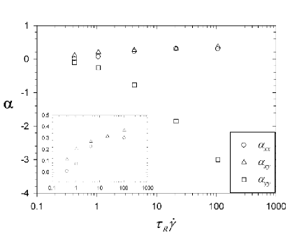
Figure 6: Plot of the thermodynamic force field, $\boldsymbol{\alpha}$, vs. De number for the C₅₀H₁₀₂ PE melt ($T$=450K, $P$=1atm). [Reproduced with permission from Baig_genericMC , Figure 1].

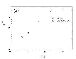
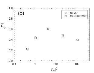
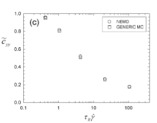
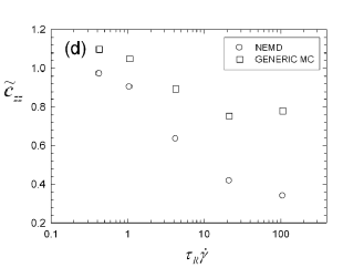
Figure 7: Comparison of the conformation tensor $\mathbf{c}$ components between NEMD and GENERIC MC simulations, as a function of De number: (a) $c_{xx}$, (b) $c_{xy}$, (c) $c_{yy}$, and (d) $c_{zz}$. The error bars are smaller than the size of the symbols. [Reproduced with permission from Baig_genericMC , Figure 1].

The information provided by the GENERIC MC simulations is important in many aspects:

• The dependence of the components of the tensor $\boldsymbol{\alpha}$ on De is directly related to the (nonequilibrium) free energy of system – see Eq. (22). Therefore, with the proposed methodology one can accurately calculate the free energy of the simulated system by requiring a series of simulations, according to the thermodynamic state points, by varying one component of $\boldsymbol{\alpha}$ and fixing the rest and then using thermodynamic integration. This can serve as a starting point for developing more accurate viscoelastic models.

• The new thermodynamically-guided method can help overcome the problem of long relaxation times (and of statistical noise in the Newtonian plateau) faced in brute-force NEMD simulations by providing the initial configuration at the relevant nonequilibrium state for a given De.

• The new method can also be combined with recently proposed coarse-graining simulation strategies for long polymer melts to enable the simulation of the viscoelastic properties of high molecular weight polymers, comparable to those encountered in practical polymer processing.

IV.3 Systematic time-scale bridging molecular dynamics for flowing polymer melts

We consider again a description of the polymer melt coarse-grained to the level of the conformation tensor. The corresponding Poisson bracket is known analytically, see Sect. IV.1. Same as in Sect. IV.2, we investigate the nonequilibrium stationary state of the polymer melt in a given flow situation, and therefore face the same problem of solving the stationary GENERIC equation (23) self-consistently. Here, we complete the studies reported in Sect. IV.2 and consistently determine also the friction matrix ${\bf M}$ from microscopic fluctuations according to general formula (10). Our presentation mainly follows Ref. pi_bemd .

IV.3.1 Systematic time-scale bridging algorithm

The coarse-grained energy and entropy, as well as the Poisson bracket require only static information and can therefore be determined very efficiently by Monte Carlo (MC) simulation methods, see Section IV.2 and Binder_MCguide ; Binder_MCMDpoly . Only the friction matrix ${\bf M}$ depends on dynamical properties, thus its numerical evaluation requires dynamical simulation, in our case Molecular Dynamics (MD). The GENERIC coarse-graining approach therefore suggests to combine the strengths of MC and MD simulations in a well-defined way to break the time-scale gap between microscopic and macroscopic scales.

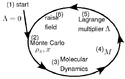
Figure 8: Schematic illustration of systematic time-scale bridging algorithm which consistently combines Monte Carlo and Molecular Dynamics simulations.

In order to implement these ideas consistently we propose a hybrid algorithm pi_bemd schematically illustrated in Fig. 8 as a general strategy for time-scale bridging simulations based on GENERIC. For the special case of flowing, unentangled polymer melts, the algorithm was implemented and tested in Ref. pi_bemd . For simplicity and speed of calculations, the classical FENE bead-spring model introduced in loose was used in these studies, although making use of an atomistic model does not pose any extra difficulties.

For this model system subject to a stationary flow with fixed velocity gradient $\boldsymbol{\kappa}$, the algorithm illustrated in Fig. 8 can be implemented as follows.

1. Start with an equilibrium system with $\boldsymbol{\kappa}=\boldsymbol{\lambda}={\bf 0}$.

2. Use a Monte Carlo scheme in order to generate an ensemble of $n_{\rm s}$ (typically $n_{\rm s}=500$) independent configurations that are distributed according to the generalized canonical distribution (16) with the current value of $\boldsymbol{\lambda}$. Calculate the value of the relevant variables in this ensemble, $\mathbf{x}=\langle\boldsymbol{\Pi}\rangle_{x}$. In order to efficiently generate an ensemble of $n_{\rm s}$ such configurations, a slight modification of the Monte Carlo algorithm proposed in mk_createchains was used in pi_bemd . The numerical values of the coarse-grained variables $\mathbf{x}=\langle\boldsymbol{\Pi}\rangle_{x}$ can then be estimated as the ensemble average $\mathbf{x}=(1/n_{\rm s})\sum_{k=1}^{n_{\rm s}}\boldsymbol{\Pi}(\mathbf{z}_{k})$ of the $n_{\rm s}$ configurations $\{\mathbf{z}_{k}\}$. In the last step, Maxwellian distributed velocities are assigned to the particles, realizing equilibrium in momentum space for the present choice of (velocity-independent) relevant variables.

3. The Monte Carlo generated ensemble is used as initial condition for Molecular Dynamics simulations of Hamilton’s microscopic dynamics. We use a standard velocity-Verlet algorithm that preserves the symplectic structure to simulate trajectories $\mathbf{z}_{k}(t)$, $k=1,\ldots,n_{\rm s}$, during a “short” time interval $0\leq t\leq\tau_{\rm s}$. The separating time scale $\tau_{\rm s}$ is short enough, such that the relevant variables $\mathbf{x}$ do not change significantly during the MD simulation. For this reason, the MD part of the simulation does not need any constraints such as thermo- or barostats nor flow-adapted boundary conditions. Performing short time, unconstrained, microcanonical molecular dynamics simulations is one of the great benefits of the present approach as it makes the scheme both highly efficient and applicable to arbitrary flow situations that – due to the lack of corresponding boundary conditions – could not be simulated so far.

4. From the particle trajectories $\mathbf{z}_{k}(t)$, we evaluate the friction matrix ${\bf M}$ from Eq. (10). We make use of time-translational invariance to equivalently rewrite Eq. (10) as

   $${\bf M}=\langle\mbox{\boldmath{$\cal M$}}(z)\rangle_{x},\quad\mbox{\boldmath{$\cal M$}}(\mathbf{z})=\frac{1}{2k_{\rm B}\tau_{\rm s}}\Delta_{\tau_{\rm s}}\boldsymbol{\Pi}(\mathbf{z})\Delta_{\tau_{\rm s}}\boldsymbol{\Pi}(\mathbf{z})$$ (28)

   where $\Delta_{\tau_{\rm s}}\boldsymbol{\Pi}(\mathbf{z})\equiv\boldsymbol{\Pi}(\mathbf{z}(\tau_{\rm s}))-\boldsymbol{\Pi}(\mathbf{z}(0))$ denotes fast fluctuations of $\boldsymbol{\Pi}$ (on the time scale $\tau_{\rm s}$). Equation (28) is more convenient for numerical evaluation than (10).

5. Updated value of the Lagrange multiplier $\boldsymbol{\lambda}$ are calculated from the stationary GENERIC equation (23) by inverting the symmetric, positive semi-definite matrix ${\bf M}$.

6. The procedure is now repeated until consistent values $\mathbf{x},{\bf M},\boldsymbol{\lambda}$ for given $\boldsymbol{\kappa}$ are obtained. Alternatively, one may use an efficient reweighting scheme if $\boldsymbol{\kappa}$ is changed only slightly and $\boldsymbol{\lambda}$ is already close to the true value $\boldsymbol{\lambda}\to\boldsymbol{\lambda}+\delta\boldsymbol{\lambda}$. Then, the explicit form of the generalized canonical distribution can be exploited to solve the nonlinear system of equations

   $${\bf 0}=\sum_{k=1}^{n_{\rm s}}\left[{\bf R}_{k}+k_{\rm B}\mbox{\boldmath{$\cal M$}}(\mathbf{z}_{k})\colon\!\delta\boldsymbol{\lambda}\right]w_{k},\;w_{k}\equiv\frac{e^{-\delta\boldsymbol{\lambda}:\boldsymbol{\Pi}(\mathbf{z}_{k})}}{\sum_{k^{\prime}}e^{-\delta\boldsymbol{\lambda}:\boldsymbol{\Pi}(\mathbf{z}_{k^{\prime}})}}$$ (29)

   for $\delta\boldsymbol{\lambda}$. This first order scheme solves the stationary GENERIC equations (23), where ${\bf R}_{k}\equiv\boldsymbol{\kappa}\cdot\boldsymbol{\Pi}(\mathbf{z}_{k})+\boldsymbol{\Pi}(\mathbf{z}_{k})\cdot\boldsymbol{\kappa}^{T}+k_{\rm B}\mbox{\boldmath{$\cal M$}}(\mathbf{z}_{k})\colon\!\boldsymbol{\lambda}$ is the error in the previous value of $\boldsymbol{\lambda}$. In a shear flow, for example, Eq. (29) represents six equations and six unknowns. The solution $\delta\boldsymbol{\lambda}$ of (29) allows one to calculate the reweighted slow variables and friction matrix, $\mathbf{x}=\sum_{k}w_{k}\boldsymbol{\Pi}(\mathbf{z}_{k})$, ${\bf M}=\sum_{k}w_{k}\mbox{\boldmath{$\cal M$}}(\mathbf{z}_{k})$, as well as updated Lagrange multipliers, $\boldsymbol{\lambda}\rightarrow\boldsymbol{\lambda}+\delta\boldsymbol{\lambda}$. Finally, the flow rate $\boldsymbol{\kappa}$ is increased, and the procedure is started again, until the control parameter space has been swept through.

With such a scheme, we establish the coarse-grained model along one-dimensional paths in the parameter space. Choosing, for example, viscometric flows of varying strength $\boldsymbol{\kappa}$ is analogous to the situation encountered in experiments.

IV.3.2 Fluctuations, separating time scale, and friction matrix

We have already emphasized several times that “fast” but correlated fluctuations give rise to dissipation on the coarse-grained level of description, which is described here by the friction matrix ${\bf M}$, Eq. (10) or (28). The notion “fast” is defined here by times $t$ smaller than the time scale $\tau_{\rm s}$, that separates the evolution of the relevant variables $\mathbf{x}$ from rapid dynamics of the remaining degrees of freedom. The existence of such a time scale (which is equivalent to the crucial assumption of time-scale separation discussed in Sect. III) is not obvious. Here, we observe that the correlation functions $C_{kl}(t)=\langle\dot{\Pi}_{k}^{\rm f}(t)\dot{\Pi}_{l}^{\rm f}(0)\rangle_{x}$ decay monotonically over a few molecular (Lennard-Jones) time units $\tau$. This shows that those fast fluctuations are indeed correlated only over short times compared to typical polymer relaxation times (which are huge relative to $\tau$). Therefore, we find that the friction matrix, which is proportional to the integral over $C(t)$, rapidly converges towards a value that is approximately independent of $\tau_{\rm s}$ in a broad range $5\leq\tau/\tau_{\rm s}\leq 50$, see Fig. 9.

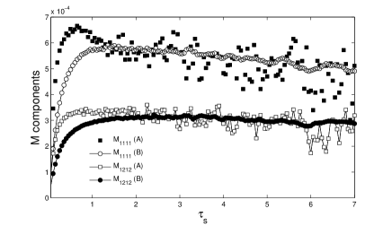
Figure 9: The friction matrix calculated from (A): Eq. (10) compared to (B): the values obtained from Eq. (28), as a function of the separating time scale $\tau_{\rm s}$. [Reprinted with permission from pi_bemd , Figure 2.]

IV.3.3 Results

Before discussing the results obtained with the proposed time-scale bridging algorithm, we like to mention several consistency checks that can be performed in order to test the range of applicability of the coarse-grained model. First, we compare two expressions for the macroscopic stress tensor. One is the standard virial expression $\boldsymbol{\sigma}=-V^{-1}\langle\mathbf{r}{\bf F}\rangle_{x}$, where $\mathbf{r}$ and ${\bf F}$ are the relative position and forces between particles. The kinetic contribution is found to be negligible in dense systems such as polymer melts as long as the flow rates are not too high mkbook . Evaluating the expression for the stress tensor $\boldsymbol{\sigma}$ in the generalized canonical ensemble leads to the expression $\boldsymbol{\sigma}^{\rm p}=-2V^{-1}k_{\rm B}T\mathbf{x}\cdot\boldsymbol{\lambda}$ for the (entropic part of the) polymer contribution to $\boldsymbol{\sigma}$, see Eq. (19). From Sect. IV.1, we know that $\boldsymbol{\sigma}$ and $\boldsymbol{\sigma}^{\rm p}$ differ by a simple-fluid contribution. Accounting for this contribution via the non-bonded short range repulsive interactions, we have verified that the two expressions for the stress tensor agree with each other for the flow rates studied. Next, by its definition and the symmetry of $\boldsymbol{\Pi}$, the matrix ${\bf M}$ possesses some basic symmetries that can be used to test the statistical accuracy of the ensemble averages. Finally, for the case of simple shear, $\boldsymbol{\kappa}=\dot{\gamma}{\bf e}_{x}{\bf e}_{y}$, we have used the identity $(x_{11}-x_{22})x_{12}^{-1}=(\lambda_{11}-\lambda_{22})\lambda_{12}^{-1}$, that can be derived from the stationary GENERIC equations Baig_genericMC , in order to check the consistency of our results. In our studies, this identity holds within error margins for the flow rates considered. We observed that breakdown of this relation at high flow rates signaled problems with the coarse-grained model as it can no longer capture the relevant dynamical processes at these elevated rates.

For the case of simple shear flow, we validated the algorithm by reproducing the chain-length dependence of the zero shear rate viscosity and of the first normal stress coefficient, which are known in the literature loose , see Fig. 10. Also the shear rate dependence of the viscosity obtained with the time-scale bridging algorithm is in very good agreement with standard NEMD results loose ; daivis ; daivis_nemd , as shown in Fig. 10.

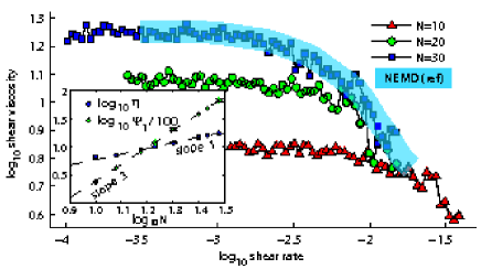
Figure 10: Polymer contribution to the shear viscosity as a function of shear rate for different molecular weights. Reference results loose obtained with standard NEMD simulations for $N=30$ are indicated. Inset: Zero shear rate viscosity $\eta_{0}$ and first normal stress coefficient $\Psi_{1}$ as a function of chain length. The expected scaling $\eta_{0}\propto N$ and $\Psi_{1}\propto N^{3}$ is observed, as shown by the dashed lines. [Reprinted with permission from pi_bemd , Figure 5.]

More results can be found in Ref. pi_bemd . As mentioned above, the flexibility of our time-scale bridging simulations allows us to study arbitrary flow fields. We therefore could perform the first steady state equibiaxial simulation for polymer melts. Results for this as well as other elongational flows can also be found in pi_bemd .

V Conclusions and perspectives

The tremendous multiplicity of length and time scales in polymeric systems clearly calls for systematic, multiscale modeling approaches in which a higher-resolution model is consistently coupled with a lower-resolution one. In particular, if one is interested in describing relaxation processes and structure development under nonequilibrium conditions, most present-day coarse-graining strategies based on the use of effective potentials are of limited use since they do not account for the additional dissipation and irreversibility accompanying inevitably the elimination of fast degrees of freedom in favor of a smaller set of slowly-relaxing structural variables. Therefore, thermodynamically guided simulations are very important and useful, where one takes full advantage of the underlying principles of nonequilibrium thermodynamics and statistical mechanics. There, the emphasis is shifted from the time evolution equations (which respect important physical laws such as the Onsager reciprocity relationships for the transport coefficients and the 2nd law of thermodynamics) to its four building blocks: the energy $E$, the entropy $S$, the Poisson matrix ${\bf L}$ and the friction matrix ${\bf M}$, describing the reversible and dissipative contributions to the dynamics.

We have outlined such a methodology for the case of unentangled polymer melts for which, guided by network theory approaches to polymer elasticity, the appropriate coarse-grained variable $\mathbf{x}$ is the conformation tensor. The underlying, microscopic model is simulated by the nonequilibrium molecular dynamics (NEMD) method. The relevant nonequilibrium state is assumed to be given by a generalized canonical distribution incorporating a conjugate variable (the Lagrange multiplier) $\boldsymbol{\lambda}$ to the conformation tensor. Monte Carlo simulations in this ensemble are employed in order to calculate the values of the slow variables $\mathbf{x}$ and the static building blocks $E$ and ${\bf L}$. For a given value of imposed flow rates, the Lagrange multiplier can be determined iteratively so that the solutions of the micro- and macro-solvers for the coarse-grained structural variables coincide. Through this one can compute model-independent values of the Lagrange multiplier, which for a wide range of strain rates (covering both the linear and the nonlinear viscoelastic regimes) bring results for the overall polymer conformation from the two models (microscale and macroscale) on top of each other. We presented two approaches to obtain the missing blocks of the macroscopic model. In Sect. IV.2, the computed values of the Lagrange multiplier are compared with those corresponding to specific choices of the friction or relaxation matrix ${\bf M}$ in the macroscopic GENERIC model (addressing the chosen structural variable; here the conformation tensor), one can identify shortcomings and suggest improvements. And this is the biggest advantage of the new framework since the multiscale model proceeds without a priori knowledge of the exact form of the macroscopic model. Being built on the GENERIC framework of nonequilibrium thermodynamics, what is only needed is just to rely on the nature of the chosen structural variables at the coarse level. This, further, emphasizes the significance of the choice of variables in the method. In the second approach, Sect. IV.3, we introduced a novel, low-noise, time-scale bridging strategy for the same system (low molecular weight, unentangled polymers) subjected to homogeneous flow fields. Through an alternating Monte Carlo-molecular dynamics iteration scheme we were able to obtain the model equations for the slow variables. For a chosen flow (including elongational ones), the method predicts structural as well as material functions beyond the regime of linear response. The method is simple to implement and allows for the calculation of time-dependent behavior through quantities readily available from the nonequilibrium steady states. In the end, it is only when all three different methodologies (macro-model, micro-model, and the macroscopic viscoelastic GENERIC equation bridging them) come together to complement each other that the entire multi-scale strategy can be considered as successful. Then, simulation techniques are elevated from brute-force computational tools to sophisticated techniques capable of mapping the detailed description of the system to a handful of carefully chosen variables whose dynamics (time evolution) is also faithfully described by an accurate analytical model.

Future efforts will address other systems such as entangled (linear and branched) polymers where, inspired by the corresponding GENERIC formalism, one should resort to a description in terms of the orientational distribution function of an entanglement segment along the primitive path of the chain.

References

- [1] J. Dealy and R. G. Larson. Structure and rheology of molten polymers. Hanser Publications, 2006.
- [2] R. B. Bird, C. F. Curtiss, R. C. Armstrong, and O. Hassager. Dynamics of Polymeric Liquids. John Wiley & Sons, New York, second edition, 1987.
- [3] R. G. Owens and T. N. Phillips. Computational Rheology. World Scientific, 2002.
- [4] R. Keunings. Advances in the computer modeling of the flow of polymeric liquids. Comp. Fluid Dyn. J., 9:449–458, 2001.
- [5] A. Ya. Malkin. The state of the art in the rheology of polymers: Achievements and challenges. Polymer Science, Ser. A, 51(1):80–102, 2009.
- [6] J. Bent, L. R. Hutchings, R. W. Richards, T. Gough, R. Spares, P. D. Coates, I. Grillo, O. G. Harlen, D. J. Read, R. S. Graham, A. E. Likhtman, D. J. Groves, T. M. Nicholson, and T. C. B. McLeish. Neutron-mapping polymer flow: Scattering, flow visualization, and molecular theory. Science, 301(5640):1691–1695, 2003.
- [7] J. Soulages, T. Schweizer, D. C. Venerus, M. Kröger, and H. C. Öttinger. Lubricated cross-slot flow of a low density polyethylene melt. J. Non-Newtonian Fluid Mech., 154:52–64, 2008.
- [8] G.W.M. Peters, J.F.M. Schoonen, F.P.T. Baaijens, and H.E.H. Meijer. On the performance of enhanced constitutive models for polymer melts in a cross-slot flow. J. Non-Newtonian Fluid Mech., 82(2-3):387–427, 1999.
- [9] W.M.H. Verbeeten, G.W.M. Peters, and F.P.T. Baaijens. Viscoelastic analysis of complex polymer melt flows using the extended Pom-Pom model. J. Non-Newtonian Fluid Mech., 108(1-3):301–326, 2002.
- [10] D. G. Hassell, D. Auhl, T. C. B. McLeish, and M. R. Mackley. The effect of viscoelasticity on stress fields within polyethylene melt flow for a cross-slot and contraction-expansion slit geometry. Rheol. Acta, 47(7):821–834, 2008.
- [11] H. C. Öttinger. Systematic coarse graining: “Four lessons and a caveat” from nonequilibrium statistical mechanics. MRS Bull., 32:936–940, 2007.
- [12] M. Kröger. Models for polymeric and anisotropic liquids, volume 675 of Lecture Notes in Physics. Springer, Berlin, 2005.
- [13] K. Kremer. Modeling soft matter. In Handbook of Materials Modeling, pages 2675–2686. Springer, 2005.
- [14] M. Doi and S. F. Edwards. The Theory of Polymer Dynamics. Oxford Universit Press, Oxford, 1986.
- [15] R. B. Bird and J. M. Wiest. Constitutive equations for polymeric liquids. Ann. Rev. Fluid Mech., 27:169–193, 1995.
- [16] R. B. Bird and H. C. Öttinger. Transport properties of polymeric liquids. Ann. Rev. Phys. Chem., 43:371–406, 1992.
- [17] E. A. Colbourn, editor. Computer Simulations of Polymers. Longman Scientific & Technical, Harlow, 1994.
- [18] K. Binder, editor. Monte Carlo and Molecular Dynamics Simulations in Polymer Science. Oxford University Press, New York, 1995.
- [19] S. C. Glotzer and W. Paul. Molecular and mesoscale simulation methods for polymer materials. Annu. Rev. Mater. Res., 32:401–436, 2002.
- [20] K. Kremer. Entangled polymers: From universal aspects to structure property relations. In N. Attig, K. Binder, H. Grubmüller, and K. Kremer, editors, Computational Soft Matter: From Synthetic Polymers to Proteins, Lecture Notes, volume 23 of NIC Series, pages 141–168. John von Neumann Institute for Computing, Jülich, 2004.
- [21] K. Kremer. Computer simulations for macromolecular science. Macromol. Chem. Phys., 204(2):257–264, 2003.
- [22] M. Kotelyanskii and D. N. Theodorou, editors. Simulation Methods for Polymers. Marcel Dekker, New York, 2004.
- [23] S. Girard and F. Müller-Plathe. Coarse-graining in polymer simulations. In Novel Methods in Soft Matter Simulations, volume 640 of Lecture Notes in Phys., pages 327–356. Springer, Berlin, 2004.
- [24] T. C. B. McLeish and R. G. Larson. Molecular constitutive equations for a class of branched polymers: The pom-pom polymer. J. Rheol., 42(1):81–110, 1998.
- [25] P. Wapperom and R. Keunings. Numerical simulation of branched polymer melts in transient complex flow using pom-pom models. J. Non-Newtonian Fluid Mech., 97(2-3):267–281, 2001.
- [26] A. E. Likhtman and R. S. Graham. Simple constitutive equation for linear polymer melts derived from molecular theory: Rolie-Poly equation. J. Non-Newtonian Fluid Mech., 114(1):1–12, 2003.
- [27] G. Ianniruberto and G. Marrucci. A simple consitutive equation for entangled polymers with chain stretch. J. Rheol., 45(6):1305–1318, 2001.
- [28] P. S. Stephanou, C. Baig, and V. G. Mavrantzas. A generalized differential constitutive equation for polymer melts based on principles of noneq uilibrium thermodynamics. J. Rheol., accepted:??, 2008.
- [29] S. Kim and S. J Karrila. Microhydrodynamics: Principles and Selected Applications. Dover Publications Inc., 2005.
- [30] S. Succi. The Lattice Boltzmann Equation for Fluid Dynamics and Beyond. Numerical Mathematics and Scientific Computation. Oxford University Press, New York, 2001.
- [31] B. Dünweg and A. J. C. Ladd. Lattice Boltzmann simulations of soft matter systems. Adv. Polym. Sci., 221:89, 2009.
- [32] R.G. Winkler, K Mussawisade, M. Ripoll, and G. Gompper. Rod-like colloids and polymers in shear flow: a multi-particle-collision dynamics study. J. Phys.: Condens. Matter, 16:S3941–S3954, 2004.
- [33] G. Gompper, T. Ihle, D.M. Kroll, and R.G. Winkler. Multi-particle collision dynamics: a particle-based mesoscale simulation approach to the hydrodynamics of complex fluids. Adv. Polym. Sci, 221:1, 2009.
- [34] C. Holm, J. F. Joanny, K. Kremer, R. R. Netz, P. Reineker, C. Seidel, T. A. Vilgis, and R. G. Winkler. Polyelectrolyte theory. In Polyelectrolytes with Defined Molecular Architecture II, volume 166 of Advances in Polymer Science, pages 67–111. Springer, 2004.
- [35] J.-E. Shea and C. L. Brooks III. From folding theories to folding proteins: A review and assessment of simulation studies of protein folding and unfolding. Ann. Rev. Phys. Chem., 52:499–535, 2001.
- [36] R. S. Graham, A. E. Likhtman, T. C. B. McLeish, and S. T. Milner. Microscopic theory of linear, entangled polymer chains under rapid deformation including chain stretch and convective constraint release. J. Rheol., 47(5):1171–1200, 2003.
- [37] D. Auhl, J. Ramirez, A. E. Likhtman, P. Chambon, and C. Fernyhough. Linear and nonlinear shear flow behavior of monodisperse polyisoprene melts with a large range of molecular weights. J. Rheol., 52(3):801–835, 2008.
- [38] G. Ianniruberto and G. Marrucci. A multi-mode CCR model for entangled polymers with chain stretch. J. Non-Newtonian Fluid Mech., 102(2):383–395, 2002.
- [39] H. C. Öttinger and A. N. Beris. Thermodynamically consistent reptation model without independent alignment. J. Chem. Phys., 110:6593–6596, 1999.
- [40] H. C. Öttinger. Thermodynamically admissible reptation models with anisotropic tube cross sections and convective constraint release. J. Non-Newtonian Fluid Mech., 89:165–185, 2000.
- [41] H. C. Öttinger. A thermodynamically admissible reptation model for fast flows of entangled polymers. J. Rheol., 43:1461–1493, 1999.
- [42] J. Fang, M. Kröger, and H. C. Öttinger. A thermodynamically admissible reptation model for fast flows of entangled polymers. II. Model predictions for shear and elongational flows. J. Rheol., 44:1293–1317, 2000.
- [43] D. W. Mead, R. G. Larson, and M. Doi. A molecular theory for fast flows of entangled polymers. Macromolecules, 31(22):7895 –7914, 1998.
- [44] J. D. Schieber, J. Neergaard, and S. Gupta. A full-chain, temporary network model with slip-links, chain-length fluctuations, chain connectivity and chain stretching. J. Rheol., 47(1):213–233, 2003.
- [45] S. Shanbhag and R. G. Larson. A slip-link model of branch-point motion in entangled polymers. Macromolecules, 37(21):8160–8166, 2004.
- [46] D. M. Nair and J. D. Schieber. Linear viscoelastic predictions of a consistently unconstrained brownian slip-link model. Macromolecules, 39(9):3386–3397, 2006.
- [47] A. E. Likhtman. Single-chain slip-link model of entangled polymers: Simultaneous description of neutron spin-echo, rheology, and diffusion. Macromolecules, 38(14):6128–6139, 2005.
- [48] M. Doi and J. Takimoto. Molecular modelling of entanglement. Philos. Trans. R. Soc. Lond. A, 361(1805):641–652, 2003.
- [49] Y. Masubuchi, J.-I. Takimoto, K. Koyama, G. Ianniruberto, G. Marrucci, and F. Greco. Brownian simulations of a network of reptating primitive chains. J. Chem. Phys., 115(9):4387–4395, 2001.
- [50] Y. Masubuchi, G. Ianniruberto, F. Greco, and G. Marrucci. Entanglement molecular weight and frequency response of sliplink networks. J. Chem. Phys., 119(13):6925–6930, 2003.
- [51] D. Rigby and B. E. Eichinger. Polymer modeling. Curr. Opinion Solid State Material Science, 5(5):445–450, 2001.
- [52] J. I. Siepmann, S. Karaborni, and B. Smit. Simulating the critical behaviour of complex fluids. Nature, 365:330–332, 1993.
- [53] P. Padilla and S. Toxvaerd. Structure and dynamical behavior of fluid n-alkanes. J. Chem. Phys., 95(1):509–519, 1991.
- [54] D. K. Dysthe, A. H. Fuchs, and B. Rousseau. Fluid transport properties by equilibrium molecular dynamics. III. Evaluation of united atom interaction potential models for pure alkanes. J. Chem. Phys., 2000.
- [55] M. Rehan, W. L. Mattics, and U. W. Suter. Rotational isomeric state models in macromolecular systems. Adv. Polym. Sci., 131-132, 1997.
- [56] R. Kubo, M. Toda, and N. Hashitsume. Statistical Physics II. Nonequilibrium Statistical Mechanics. Springer, Berlin, second edition, 1991.
- [57] M. Vladkov and J.-L. Barrat. Linear and nonlinear viscoelasticity of unentangled polymer melts: Molecular dynamics and Rouse mode analysis. Macromol. Theory Simul., 15:252–262, 2006.
- [58] J. T. Padding and W. J. Briels. Ab-initio coarse-graining of entangled polymer systems. In Nanostructured Soft Matter, NanoScience and Technology, pages 437–460. Springer, Netherlands, 2007.
- [59] K. Kremer and G.S. Grest. Dynamics of entangled linear polymer melts: A molecular-dynamics simulation. J. Chem. Phys., 92:5057–5086, 1990.
- [60] M. Kröger, W. Loose, and S. Hess. Structural changes and rheology of polymer melts via nonequilibrium molecular dynamics. J. Rheol., 37:1057, 1993.
- [61] B. D. Todd. Computer simulation of simple and complex atomistic fluids by nonequilibrium molecular dynamics techniques. Comp. Phys. Comm., pages 14–21, 2001.
- [62] B. D. Todd and P. J. Daivis. Homogeneous non-equilibrium molecular dynamics simulations of viscous flow: techniques and applications. Mol. Sim., 33:189, 2007.
- [63] M. Kröger and S. Hess. Rheological evidence for a dynamical crossover in polymer melts via nonequilibrium molecular dynamics. Phys. Rev. Lett., 85:1128–1131, 2000.
- [64] B. J. Edwards, C. Baig, and D. J. Keffer. An examination of the validity of nonequilibrium molecular-dynamics simulation algorithms for arbitrary steady-state flows. J. Chem. Phys., 123:114106, 2005.
- [65] B. J. Edwards, C. Baig, and D. J. Keffer. A validation of the p-SLLOD equations of motion for homogeneous steady-state flows. J. Chem. Phys., 124:194104, 2006.
- [66] C. Baig, B. J. Edwards, D. J. Keffer, and H. D. Cochran. A proper approach for nonequilibrium molecular dynamics simulations of planar elongational flow. J. Chem. Phys., 112:114103, 2005.
- [67] C. Baig, B. J. Edwards, D. J. Keffer, H. D. Cochran, and V. A. Harmandaris. Rheological and structural studies of linear polyethylene melts under planar elongational flow using nonequilibrium molecular dynamics simulations. J. Chem. Phys., 124:084902, 2006.
- [68] A. W. Lees and S. F. Edwards. The computer study of transport processes under extreme conditions. J. Phys. C, 5(15):1921–1930, 1972.
- [69] A. M. Kraynik and D. A. Reinelt. Extensional motions of spatially periodic lattices. Int. J. Multiphase Flow, 18(6):1045–1059, 1992.
- [70] M. Doi. Challenge in polymer physics. Pure Appl. Chem., 75(10):1395–1402, 2003.
- [71] W. Paul, G. D. Smith D. Y., Yoon, B. Farago, S. Rathgeber, A. Zirkel, L. Willner, and D. Richter. Chain motion in an unentangled polyethylene melt: A critical test of the Rouse model by molecular dynamics simulations and neutron spin echo spectroscopy. Phys. Rev. Lett., 80(11):2346–2349, 1998.
- [72] S. Bair, C. McCabe, and P. T. Cummings. Comparison of nonequilibrium molecular dynamics with experimental measurements in the nonlinear shear-thinning regime. Phys. Rev. Lett., 88:058302, 2002.
- [73] R. E. Tuzun, D. W. Noid, B. G. Sumpter, and C. E. Wozny. Recent advances in polymer molecular dynamics simulation and data analysis. Macromol. Theor. Simul., 6(5):855–880, 2003.
- [74] C. K. Ober, S. Z. D. Cheng, P. T. Hammond, M. Muthukumar, E. Reichmanis, K. L. Wooley, and T. P. Lodge. Research in macromolecular science: Challenges and opportunities for the next decade. Macromolecules, 42:465–471, 2009.
- [75] V. G. Mavrantzas, T. Boone, E. Zervopoulou, and D. N. Theodorou. End-bridging Monte Carlo: An ultra-fast algorithm for the equilibration of the condensed phases of long polymers. Macromolecules, 32:5072–5096, 1999.
- [76] V. G. Mavrantzas. Monte Carlo simulation of chain molecules. In S. Yip, editor, Handbook of Materials Modeling, pages 2583–2597. Springer, Netherlands, 2005.
- [77] N. Ch. Karayiannis, V. G. Mavrantzas, and D. N. Theodorou. A novel Monte Carlo scheme for the rapid equilibration of atomistic model polymer systems of precisely defined molecular architecture. Phys. Rev. Lett., 88:105503, 2002.
- [78] R. Auhl, R. Everaers, G. S. Grest, and K. Kremer. Equilibration of long chain polymer melts in computer simulations. J. Chem. Phys., page 12718, 2003.
- [79] D. N. Theodorou. Equilibration and coarse-graining methods for polymers. In Computer Simulations in Condensed Matter Systems: From Materials to Chemical Biology, Volume 2, volume 704 of Lecture Notes in Physics, pages 419–448. Springer, Berlin, 2006.
- [80] M. Kröger. Shortest multiple disconnected path for the analysis of entanglements in two- and three-dimensional polymeric systems. Comp. Phys. Comm., 168(3):209–232, 2005.
- [81] S. K. Sukumaran, G. S. Grest, K. Kremer, and R. Everaers. Identifying the primitive path mesh in entangled polymer liquids. J. Poly. Sci. B: Poly. Phys., 43(8):917–933, 2005.
- [82] R. Everaers, S. K. Sukumaran, G. S. Grest, C. Svaneborg, A. Sivasubramanian, and K. Kremer. Rheology and microscopic topology of entangled polymeric liquids. Science, 303:823–826, 2004.
- [83] S. Shanbhag, S. J. Park, W. Zhou, and R. G. Larson. Implications of microscopic simulations of polymer melts for mean-field tube theories. Mol. Sim., 105(2-3):249–260, 2007.
- [84] M. Kröger, J. Ramírez, and H. C. Öttinger. Projection from an atomistic chain contour to its primitive path. Polymer, 43:477–487, 2002.
- [85] V. A. Harmandaris, V. G. Mavrantzas, D. N. Theodorou, M. Kröger, J. Ramírez, H. C. Öttinger, and D. Vlassopoulos. Crossover from the Rouse to the entangled polymer melt regime: Signals from long, detailed atomistic molecular dynamics simulations, supported by rheological experiments. Macromolecules, 36:1376–1387, 2003.
- [86] J. M. Kim, D. J. Keffer, M. Kröger, and B. J. Edwards. Rheological and entanglement characteristics of linear-chain polyethylene liquids in planar Couette and planar elongational flows. J. Non-Newtonian Fluid Mech., 152:168–183, 2008.
- [87] R. E. Miller and E. B. Tadmor. Hybrid continuum mechanics and atomistic methods for simulating materials deformation and failure. MRS Bull., 32:920–926, 2007.
- [88] G. Lu, E. B. Tadmor, and E. Kaxiras. From electrons to finite elements: A concurrent multiscale approach for metals. Phys. Rev. B, 73:024108, 2008.
- [89] G. De Fabritiis, R. Delgado-Buscalioni, and P. V. Coveney. Multiscale modeling of liquids with molecular specificity. Phys. Rev. Lett., 97:134501, 2006.
- [90] S. T. Milner. Polymer brushes. Science, 251(4996):905–914, 1991.
- [91] M. G. Guenza. Theoretical models for bridging timescales in polymer dynamics. J. Phys.: Condens. Matter, 20:033101, 2008.
- [92] M. Praprotnik, C. Junghans, L. D. Site, and K. Kremer. Simulation approaches to soft matter: Generic statistical properties vs. chemical details. Comp. Phys. Comm., 179(1-3):51–60, 2008.
- [93] M. Praprotnik, L. D. Site, and K. Kremer. Multiscale simulation of soft matter: From scale bridging to adaptive resolution. Ann. Rev. Phys. Chem., 59:545–571, 2008.
- [94] K. Kremer and F. Müller-Plathe. Multiscale simulation in polymer science. Mol. Sim., 28:729–750, 2002.
- [95] J. Baschnagel, K. Binder, P. Doruker, A.A. Gusev, O. Hahn, K. Kremer, W.L. Mattice, F. Müller-Plathe, M. Murat, W. Paul, S. Santos, U.W. Suter, and V. Tries. Bridging the gap between atomistic and coarse-grained models of polymers: Status and perspectives. Adv. Polym. Sci., 152:41–156, 2000.
- [96] P. Nielaba, M. Mareschal, and G. Cicotti, editors. Bridging Time Scales: Molecular Simulations for the Next Decade, volume 606 of Lecture Notes in Physics. Springer, Berlin, 2002.
- [97] E. Weinan, X. Li, and E. Vanden-Eijnden. Some recent progress in multiscale modeling. In S. Attinger and P. Koumoutsakos, editors, Multiscale Modelling and Simulation, volume 39 of Lecture Notes in Computational Science and Engineering, pages 3–23. Springer, 2004.
- [98] G. A. Voth, editor. Coarse-Graining of condensed phases and biomolecular systems. CRC press, Boca Raton, 2009.
- [99] T. Murtola, A. Bunker, I. Vattulainen, M. Deserno, and M. Karttunen. Multiscale modeling of emergent materials: biological and soft matter. Phys. Chem. Chem. Phys., 11(12):1869–1892, 2009.
- [100] A. R. Denton. Effective interactions in soft materials. In Nanostructured Soft Matter, NanoScience and Technology, pages 395–433. Springer, Netherlands, 2007.
- [101] R. Faller. Coarse-grain modeling of polymers. In T. R. Cundari K. B. Lipkowitz, editor, Reviews in Computational Chemistry, volume 23, pages 233–262. John Wiley & Sons, Inc., 2007.
- [102] A. N. Gorban, N. K. Kazantzis, I. V. Kevrekidis, H. C. Öttinger, and C. Theodoropoulos, editors. Model Reduction and Coarse-Graining Approaches for Multiscale Phenomena. Springer, Berlin, 2006.
- [103] H. Grabert. Projection Operator Techniques in Nonequilibrium Statistical Mechanics. Springer, Berlin, 1982.
- [104] S.O. Nielsen, C.F. Lopez, G. Srinivas, and M.L. Klein. Coarse grain models and the computer simulation of soft materials. J. Phys.: Condens. Matter, 16:R481, 2004.
- [105] J. P. Hansen and H. Löwen. Effective interactions for large-scale simulations of complex fluids. In P. Nielaba, M. Mareschal, and G. Cicotti, editors, Bridging Time Scales: Molecular Simulations for the Next Decade, pages 167–196. Springer, Berlin, 2002. Lecture Notes in Physics, Vol. 606.
- [106] Q. Sun and R. Faller. Systematic coarse-graining of atomistic models for simulation of polymeric systems. Comp. Chem. Eng., 29(11-12):2380–2385, 2005.
- [107] R. Faller. Automatic coarse graining of polymers. Polymer, 45(11):3869–3876, 2004.
- [108] T. Spyriouni, C. Tzoumanekas, D.N. Theodorou, F. Müller-Plathe, and G. Milano. Coarse-grained and reverse-mapped united-atom simulations of long-chain atactic polystyrene melts: Structure, thermodynamic properties, chain conformation, and entanglements. Macromolecules, 40:3876–3885, 2007.
- [109] K. Kamio, K. Moorthi, and D.N. Theodorou. Coarse grained end bridging Monte Carlo simulations of poly(ethylene terephthalate) melt. Macromolecules, 40:710–722, 2007.
- [110] D. Reith, M. Pütz, and F. Müller-Plathe. Deriving effective mesoscale potentials from atomistic simulations. J. Comp. Chem., 24(13):1624–1636, 2003.
- [111] D. Reith, H. Meyer, and F. Müller-Plathe. Mapping atomistic to coarse-grained polymer models using automatic simplex optimization to fit structural properties. Macromolecules, 34(7):2335–2345, 2001.
- [112] G. Milano and F. Müller-Plathe. Mapping atomistic simulations to mesoscopic models: A systematic coarse-graining procedure for vinyl polymer chains. J. Phys. Chem. B, 109:18609–18619, 2005.
- [113] G. Santangelo, A. Di Matteo, F. Müller-Plathe, and G. Milano. From mesoscale back to atomistic models: A fast reverse-mapping procedure for vinyl polymer chains. J. Phys. Chem. B, 111:2765–2773, 2007.
- [114] V. A. Harmandaris, D. Reith, N. F. A. van der Vegt, and K. Kremer. Comparison between coarse-graining models for polymer systems: Two mapping schemes for polystyrene. Macromol. Chem. Phys., 208(19-20):2109–2120, 2007.
- [115] V. A. Harmandaris, N.P. Adhikari, N. F. A. van der Vegt, and K. Kremer. Hierarchical modeling of polystyrene: From atomistic to coarse-grained simulations. Macromolecules, 39:6708–6719, 2006.
- [116] C.F. Abrams and K. Kremer. Combined coarse-grained and atomistic simulation of liquid bisphenol A-polycarbonate: Liquid packing and intramolecular structure. Macromolecules, 36(1):260–267, 2003.
- [117] S. Leo, N. van der Vegt, L. Delle Site, and K. Kremer. Bisphenol A polycarbonate: Entanglement analysis from coarse-grained MD simulations. Macromolecules, 38:8078–8092, 2005.
- [118] P. Carbone, F. Negri, and F. Müller-Plathe. Coarse-grained model for polyphenylene dendrimers: Switching and backfolding of planar three-fold core dendrimers. Macromolecules, 40(19):7044–7055, 2007.
- [119] T. A. Knotts IV, N. Rathore, D.C. Schwartz, and J. J. de Pablo. A coarse grain model for DNA. J. Chem. Phys., 126:084901, 2007.
- [120] C. Peter, L. D. Site, and K. Kremer. Classical simulations from the atomistic to the mesoscale and back: coarse graining an azobenzene liquid crystal. Soft Matter, 4:859–869, 2008.
- [121] J. Zwicker and R.J. Lovett. When does a pair correlation function fix the state of an equilibrium system? J. Chem. Phys., 93:6752–6755, 1990.
- [122] A. K. Soper. Empirical potential Monte Carlo simulation of fluid structure. Chemical Physics, 202(2):295–306, 1996.
- [123] H.-J. Qian, C. C. Liewb, and F. Müller-Plathe. Effective control of the transport coefficients of coarse-grained liquid and polymer models using the dissipative particle dynamics and Lowe-Andersen equations of motion. preprint, 2009.
- [124] X. Chen, P. Carbone, W. L. Cavalcanti, G. Milano, and F. Müller-Plathe. Viscosity and structural alteration of a coarse-grained model of polystyrene under steady shear flow studied by reverse nonequilibrium molecular dynamics. Macromolecules, 40:8087–8095, 2007.
- [125] P. K. Depa and J. K. Maranas. Speed up of dynamic observables in coarse-grained molecular-dynamics simulations of unentangled polymers. J. Chem. Phys., 123(094901), 2005.
- [126] V. A. Harmandaris and K. Kremer. Quantitative study of polymer dynamics through hierarchical multi-scale dynamic simulations. cond-mat, arXiv:0809.1518, 2008.
- [127] W.G. Noid, J.-W. Chu, G.S. Ayton, V. Krishna, S. Izvekov, G.A. Voth, A. Das, and H.C. Andersen. The multiscale coarse-graining method. I. A rigorous bridge between atomistic and coarse-grained models. J. Chem. Phys., 128:244114, 2008.
- [128] W.G. Noid, P. Liu, Y. Wang, J.-W. Chu, G.S. Ayton, S. Izvekov, H.C. Andersen, and G.A. Voth. The multiscale coarse-graining method. II. Numerical implementation for coarse-grained molecular models. J. Chem. Phys., 128:244115, 2008.
- [129] R.L. Henderson. Uniqueness theorem for fluid pair correlation-functions. Phys. Lett. A, 49(3):197–198, 1974.
- [130] C.G. Gray and K.E. Gubbins. Theory of Molecular Fluids. Oxford University Press, New York, 1984.
- [131] S. Jain, S. Garde, and S.K. Kumar. Do inverse Monte Carlo algorithms yield thermodynamically consistent interaction potentials? Ind. Eng. Chem. Res., 45:5614–5618, 2006.
- [132] P. Carbone, H. A. K. Varzaneh, X. Chen, and F. Müller-Plathe. Transferability of coarse-grained force fields: The polymer case. J. Chem. Phys., 128:064904, 2008.
- [133] V. Krishna, W.G. Noid, and G.A. Voth. The multiscale coarse-graining method. IV. Transferring coarse-grained potentials between temperatures. J. Chem. Phys., 131(2):024103, 2009.
- [134] Y. Wang, W. G. Noid, P. Liu, and G. A. Voth. Effective force coarse-graining. Phys. Chem. Chem. Phys, 11(12):2002–2015, 2009.
- [135] X. Guerrault, B. Rousseau, and J. Farago. Dissipative particle dynamics simulations of polymer melts. I. Building potential of mean force for polyethylene and cis-polybutadiene. J. Chem. Phys., 121:6538–6546, 2004.
- [136] J. T. Padding and W. J. Briels. Coarse-grained molecular dynamics simulations of polymer melts in transient and steady shear flow. J. Chem. Phys., 118(22):10276–10286, 2003.
- [137] J. T. Padding and W. J. Briels. Uncrossability constraints in mesoscopic polymer melt simulations: Non-Rouse behavior of C120H242. J. Chem. Phys., 115(6):2846–2859, 2001.
- [138] R. L. C. Akkermans and W. J. Briels. A structure-based coarse-grained model for polymer melts. J. Chem. Phys., 114(2):1020–1031, 2001.
- [139] R. L. C. Akkermans and W. J. Briels. Coarse-grained dynamics of one chain in a polymer melt. J. Chem. Phys., 113(15):6409–6422, 2000.
- [140] D.J. Evans and G.P. Morriss. Nonlinear-response theory for steady planar Couette flow. Phys. Rev. A, 30:1528–1530, 1984.
- [141] P. Kindt and W.J. Briels. Scaling of mesoscale simulations of polymer melts with the bare friction coefficient. J. Chem. Phys., 123:224903, 2005.
- [142] H. C. Öttinger. Coarse-graining of wormlike polymer chains for substantiating reptation. J. Non-Newtonian Fluid Mech., 120:207–213, 2004.
- [143] C. Tzoumanekas and D.N. Theodorou. Topological analysis of linear polymer melts: A statistical approach. Macromolecules, 39:4592–4604, 2006.
- [144] G. Tsolou, V.G. Mavrantzas, and D.N. Theodorou. Detailed atomistic molecular dynamics simulation of cis-1,4-poly(butadiene). Macromolecules, 38:1478–1492, 2005.
- [145] K. Kremer, S.K. Sukumaran, R. Everaers, and G.S. Grest. Entangled polymer systems. Comp. Phys. Comm., 169:75–81, 2005.
- [146] N. Uchida, G.S. Grest, and R. Everaers. Viscoelasticity and primitive path analysis of entangled polymer liquids: From F-actin to polyethylene. J. Chem. Phys., 128:044902, 2008.
- [147] K. Foteinopoulou, N.C. Karayiannis, V.G. Mavrantzas, and M. Kröger. Primitive path identification and entanglement statistics in polymer melts: Results from direct topological analysis on atomistic polyethylene models. Macromolecules, 39:4207–4216, 2006.
- [148] R.N. Khaliullin and J.D. Schieber. Analytic expressions for the statistics of the primitive-path length in entangled polymers. Phys. Rev. Lett., 100:188302, 2008.
- [149] M. Doi and N.Y. Kuzuu. Rheology of star polymers in concentrated solutions and melts. J. Polym. Sci., Polym. Lett. Ed., 18:775–780, 1980.
- [150] S. Shanbhag and R. G. Larson. Chain retraction potential in a fixed entanglement network. Phys. Rev. Lett., 94:076001, 2005.
- [151] M. Doi and S. F. Edwards. Dynamics of concentrated polymer systems. Part 2. – Molecular motion under flow. J. Chem. Soc. Faraday Trans. 2, 74:1802–1817, 1978.
- [152] M. Doi and J.-I. Takimoto. Molecular modelling of entanglement. Phil. Trans. R. Soc. Lond. A, 361:641–652, 2003.
- [153] T. Yaoita, T. Isaki, Y. Masubuchi, H. Watanabe, G. Ianniruberto, F. Greco, and G. Marrucci. Highly entangled polymer primitive chain network simulations based on dynamic tube dilation. J. Chem. Phys., 121(24):12650–12654, 2004.
- [154] Y. Masubuchi, G. Ianniruberto, F. Greco, and G. Marrucci. Quantitative comparison of primitive chain network simulations with literature data of linear viscoelasticity for polymer melts. J. Non-Newtonian Fluid Mech., 149:87–92, 2008.
- [155] A. A. Louis, P. G. Bolhuis, R. Finken, V. Krakoviack, E. J. Meijer, and J. P. Hansen. Coarse-graining polymers as soft colloids. Physica A, 306:251–261, 2002.
- [156] A. A. Louis, P. G. Bolhuis, J. P. Hansen, and E. J. Meijer. Can polymer coils be modeled as “soft colloids”? Phys. Rev. Lett., 85:2522, 2000.
- [157] P. G. Bolhuis, A. A. Louis, J. P. Hansen, and E. J. Meijer. Accurate effective pair potentials for polymer solutions. J. Chem. Phys., 114:4296, 2001.
- [158] P. Kindt and W.J. Briels. A single particle model to simulate the dynamics of entangled polymer melts. J. Chem. Phys., 127(13):134901, 2007.
- [159] I. Pagonabarraga and D. Frenkel. Non-ideal DPD fluids. Mol. Simul., 25:167–175, 2000.
- [160] I. Pagonabarraga and D. Frenkel. Dissipative particle dynamics for interacting systems. J. Chem. Phys., 115(11):5015–5026, 2001.
- [161] V.G. Mavrantzas and D.N. Theodorou. Atomistic simulation of polymer melt elasticity: Calculation of the free energy of an oriented polymer melt. Macromolecules, 31(18):6310–6332, 1998.
- [162] A. van den Noort, W.K. den Otter, and W.J. Briels. Coarse-graining of slow variables in dynamic simulations of soft matter. Europhys. Lett., 80:28003, 2007.
- [163] A. van den Noort and W.J. Briels. Coarse grained simulations of elongational viscosities, superposition rheology and shear banding in model core-shell systems. Macromol. Theory Simul., 16(8):742–754, 2008.
- [164] V. G. Mavrantzas and H. C. Öttinger. Atomistic Monte Carlo simulations of polymer melt elasticity: Their nonequilibrium thermodynamics GENERIC formulation in a generalized canonical ensemble. Macromolecules, 35:960–975, 2002.
- [165] F. E. Bernardin III and G. C. Rutledge. Estimation of macromolecular configurational properties from atomistic simulations of oligomers under nonequilibrium conditions. Macromol. Theor. Simul., 17:23–31, 2008.
- [166] H. C. Öttinger. Thermodynamic admissibility of the pompon model for branched polymers. Rheol. Acta, 40:317–321, 2001.
- [167] H. C. Öttinger. Beyond Equilibrium Thermodynamics. Wiley, Hoboken, 2005.
- [168] P.J. Hoogerbrugge and J.M.V.A. Koelman. Simulating microscopic hydrodynamic phenomena with dissipative particle dynamics. Europhys. Lett., 19(3):155–160, 1992.
- [169] M. Fyta, J. Sircar, E. Kaxiras, S. Melchionna, M. Bernaschi, and S. Succi. Parallel multiscale modeling of biopolymer dynamics with hydrodynamic correlations. Int. J. Multiscale Comp. Eng., 6(1):25, 2008.
- [170] M. Ripoll, K. Mussawisade, R. G. Winkler, and G. Gompper. Low-Reynolds-number hydrodynamics of complex fluids by multi-particle-collision dynamics. Europhys. Lett., 68:106, 2004.
- [171] T. Ihle, E. Tüzel, and D. M. Kroll. Consistent particle-based algorithm with a non-ideal equation of state. Europhys. Lett., 73:664, 2006.
- [172] J. T. Padding and W. J. Briels. Time and length scales of polymer melts studied by coarse-grained molecular dynamics simulations. J. Chem. Phys., 117(2):925–943, 2002.
- [173] H. C. Öttinger. General projection operator formalism for the dynamics and thermodynamics of complex fluids. Phys. Rev. E, 57:1416, 1998.
- [174] P. M. Chaikin and T. C. Lubensky. Principles of Condensed Matter Physics. Cambridge University Press, 2000.
- [175] A. N. Beris and B. J. Edwards. Thermodynamics of Flowing Systems with Internal Microstructure. Oxford University Press, New York, 1994.
- [176] P. Español. Statistical mechanics of coarse-graining. In Novel Methods in Soft Matter Simulations, volume 640 of Lecture Notes in Physics, pages 69–115. Springer, 2004.
- [177] J.J. de Pablo and H. C. Öttinger. An atomistic approach to general equation for the nonequilibrium reversible-irreversible coupling. J. Non-Newtonian Fluid Mech., 96:137–162, 2001.
- [178] H. C. Öttinger and H. Struchtrup. The mathematical procedure of coarse graining: From Grad’s ten-moment equations to hydrodynamics. Multiscale Model. Simul., 6:53–69, 2007.
- [179] I. E. Dzyaloshinskii and G. E. Volovick. Poisson brackets in condensed matter physics. Ann. Phys. (N.Y.), 125(1):67–97, 1980.
- [180] R. K. P. Zia and B. Schmittmann. A possible classification of nonequilibrium steady states. J. Phys. A: Math. Gen., 39(24):L407–L413, 2006.
- [181] E. T. Jaynes. Information theory and statistical mechanics. Phys. Rev. A, 106(4):620–630, 1957.
- [182] D. Zubarev, V. Morozov, and G. Röpke. Statistical mechanics of nonequilibrium processes. Akademie Verlag, Berlin, 1997.
- [183] A. N. Gorban and I. V. Karlin. Invariant Manifolds for Physical and Chemical Kinetics, volume 660 of Lecture Notes in Phys. Springer, Berlin, 2005.
- [184] C. Hijón, M. Serrano, and P. Español. Markovian approximation in a coarse-grained description of atomic systems. J. Chem. Phys., 125:204101, 2006.
- [185] K. S. Schweizer. Microscopic theory of the dynamics of polymeric liquids: General formulation of a mode-mode coupling approach. J. Chem. Phys., 91(9):5802–5821, 1989.
- [186] S.-H. Chong and M. Fuchs. Mode-coupling theory for structural and conformational dynamics of polymer melts. Phys. Rev. Lett., 88:185702, 2002.
- [187] H. C. Öttinger. Nonequilibrium thermodynamics of glasses. Phys. Rev. E, 74:011113, 2006.
- [188] E. Del Gado, P. Ilg, M. Kröger, and H. C. Öttinger. Non-affine deformations of inherent structure as signature of cooperativity in supercooled liquids. Phys. Rev. Lett., 101:095501, 2008.
- [189] F. E. Bernardin III and G. C. Rutledge. Simulation of mechanical properties of oriented glassy polystyrene. Polymer, 48:7211–7220, 2007.
- [190] P. Ilg. Macroscopic thermodynamics of flowing polymers derived from systematic coarse-graining procedure. Physica A, 387:6484–6496, 2008.
- [191] M. Dressler, B. J. Edwards, and H. C. Öttinger. Macroscopic thermodynamics of flowing polymeric liquids. Rheol. Acta, 38:117–136, 1999.
- [192] M. Kröger, C. Luap, and R. Muller. Polymer melts under uniaxial elongational flow: stress-optical behavior from experiments and nemd computer simulations. Macromolecules, 30:526–539, 1997.
- [193] C. Baig and V. G. Mavrantzas. Thermodynamically guided nonequilibrium Monte Carlo method for generating realistic shear flows in polymeric systems. Phys. Rev. Lett., 99:257801, 2007.
- [194] T. C. Ionescu, B. J. Edwards, D. J. Keffer, and V. G. Mavrantzas. Energetic and entropic elasticity of nonisothermal flowing polymers: experiment, theory, and simulation. J. Rheol., 52(1):105–140, 2008.
- [195] T. C. Ionescu, B. J. Edwards, D. J. Keffer, and V. G. Mavrantzas. Atomistic simulation of energetic and entropic elasticity in short-chain polyethylenes. J. Rheol., 52(2):567–602, 2008.
- [196] C. Baig and V. G. Mavrantzas. Multiscale simulation of polymer melt viscoelasticity guided from nonequilibrium statistical thermodynamics: Atomistic non-equilibrium molecular dynamics coupled with Monte Carlo in an expanded statistical ensemble. Phys. Rev. B, 79:144302, 2009.
- [197] P. Ilg, H. C. Öttinger, and M. Kröger. Systematic time-scale-bridging molecular dynamics applied to flowing polymer melts. Phys. Rev. E, 79:011802, 2009.
- [198] D. P. Landau and K. Binder. A Guide to Monte Carlo Simulations in Statistical Physics. Cambridge University Press, 2000.
- [199] M. Kröger. Efficient hybrid algorithm for the dynamic creation of semiflexible polymer solutions, brushes, melts and glasses. Comput. Phys. Commun., 118:278–298, 1999.
- [200] P. J. Daivis, M. L. Matin, and B. D. Todd. Nonlinear shear and elongational rheology of model polymer melts at low strain rates. J. Non-Newtonian Fluid Mech., 147(1-2):35–44, 2007.
- [201] P. J. Daivis, M. L. Matin, and B. D. Todd. Nonlinear shear and elongational rheology of model polymer melts by non-equilibrium molecular dynamics. J. Non-Newtonian Fluid Mech., 111(1):1–18, 2003.