Attractor period distribution for critical Boolean networks

Abstract

Using analytic arguments, we show that dynamical attractor periods in large critical Boolean networks are power-law distributed. Our arguments are based on the method of relevant components, which focuses on the behavior of the nodes that control the dynamics of the entire network and thus determine the attractors. Assuming that the attractor period is equal to the least common multiple of the size of all relevant components, we show that the distribution in large networks is well approximated by a power-law with an exponent of $-1$. Numerical evidence based on sampling of attractors supports the conclusions of our analytic arguments.

Boolean networks have been extensively studied as simplified models for complex systems of multiple interacting units Albert and Barabási (2002); Aldana-Gonzalez et al. (2003); Drossel (2008). They are defined by a directed graph in which the nodes have binary output states that are determined by Boolean functions of the states of the nodes connected to them with directed in-links. They have been used to model a variety of biological, physical, and social systems. In a number of recent studies Li et al. (2004); Albert and Othmer (2003); Davidich and Bornholdt (2008), for example, it has been shown that Boolean network models can correctly reproduce essential features of the dynamics of real biological networks, while dramatically limiting the number of parameters needed to describe their behavior Bornholdt (2005).

In their original variant, the out-links of the directed graph that describes the topology of Boolean networks were assumed to be completely random. Of course, the topology of the interactions in real networks is far from being random. Nevertheless, the extreme abstraction of random Boolean networks allows for the identification of basic mathematical laws of complex network dynamics. Many non-trivial effects occur in this seemingly trivial model. Only recently major progress has been made toward analytically understanding the dynamics of random Boolean networks Samuelsson and Troein (2003); Drossel (2005); Mihaljev and Drossel (2006); Drossel et al. (2005).

Here we study the dynamical attractor distribution of critical Boolean networks using the method of relevant components. Numerical evidence is presented that supports our analytic arguments. Additionally, we show that the attractor distributions occurring in Boolean networks that have evolved to criticality based on a competition between nodes Paczuski et al. (2000); Bassler et al. (2004); Liu and Bassler (2007) match those we can deduce from the analytical understanding how attractors arise.

Consider ensembles of networks with $N$ nodes in which the behavior each node depends on exactly $K$ other nodes. Thus, each node of the directed graph defining the network interactions has exactly $K$ in-links. The Boolean states of the nodes are updated synchronously at uniformly spaced time steps that can be assumed to be of unit duration. Each node $i$ has a Boolean state $s_{i}(t)\in\{0,1\}$ at time $t$ that is determined by a Boolean function $f_{i}$ of the states of the $K$ nodes it depends on $i_{1}$, $i_{2}$, …$i_{K}$ had during the previous time step

$$s_{i}(t+1)=f_{i}\left(s_{i_{1}}(t),s_{i_{2}}(t),\ldots,s_{i_{K}}(t)\right),\qquad\forall i.$$ (1)

The choice of the functions $f_{i}$ determines the dynamics. A particular directed graph together with the Boolean functions defined at each node is a network realization, and so we consider consider ensembles of network realizations.

The network state of a given realization at time $t$ is the vector of $N$ Boolean components given by the states of the nodes at that time, $\vec{s}(t)$. There are $2^{N}$ possible network states. The networks we consider, therefore, have a finite state space and a discrete, deterministic dynamics. Thus, starting from any initial state the dynamics of the network state will, in finite time, collapse to an attractor of finite period. There can be one, or more, attractors, each of which has a basin of attraction corresponding to the region of state space from which the dynamics eventually collapses to that attractor. The late time dynamics of a Boolean network can be quantified by the number of attractors $\nu$, their periods $L_{j}$, and the size of their basins of attraction $A_{j}$, $j=1,2,\ldots,\nu$.

Generally, depending on the sets of Boolean functions describing the dynamics of the nodes ${\cal F}=\{f_{1},f_{2},\ldots,f_{N}\}$ in the realizations of an ensemble of networks, the dynamics of the ensemble can be classified into two phases with distinct behavior. We want to focus on the boundary between the phases, where the dynamics is critical. A critical network can be obtained either by construction, by evolving the set ${\cal F}$ of Boolean functions Bassler et al. (2004); Paczuski et al. (2000); Liu and Bassler (2007) or by evolving the topology Bornholdt and Rohlf (2000); Liu and Bassler (2006); Gross and Blasius (2008); Luque et al. (2001). Note though that evolving the Boolean functions can effectively result in an evolution of the topology Reichhardt and Bassler (2007).

The paper is organized as follows: First, we introduce some needed concepts and briefly review what is currently known about the attractor distribution of critical Boolean networks. These prior results are all numerical. Second, the attractor period distribution is calculated using novel analytic methods. As we will see, consistent with previous numerical observations, the attractor periods in large critical Boolean networks are power-law distributed. Finally, numerical results, obtained using novel methods, are shown that confirm our analytic predictions and allow some of the previous numerical results to be explained.

It is possible to distinguish the two phases of the dynamics in random Boolean networks by considering the sensitivity of the dynamical trajectory of the network state to a small change Aldana-Gonzalez et al. (2003); Derrida and Pomeau (1986); Shmulevich and Kauffman (2004). Consider two different initial states of a single network realization, $\vec{s}^{(1)}(0)$ and $\vec{s}^{(2)}(0)$. The normalized Hamming distance $h_{t}$ between subsequent trajectories of the two states is the fraction of nodes having a different node value: $h(t)=N^{-1}\sum_{i=1}^{N}\left(s_{i}^{(1)}(t)-s_{i}^{(2)}(t)\right)^{2}$. For small $h(t)$ the probability that more than one input of a node differs in the two states can be neglected and the time evolution of the Hamming distance can be written as $h(t+1)=\lambda h(t)$ where $\lambda$ is the sensitivity Shmulevich and Kauffman (2004).

The “frozen” phase of the dynamics is characterized by small sensitivities, $\lambda<1$. In this case, a perturbation of a node’s value propagates to less than one other node on average per time step. In this phase, in a large network, the output states of the vast majority of nodes become frozen and a perturbation of a node’s value will eventually die out. A node is “frozen” on an attractor if it stops changing its value after some transient time. The number and periods of the attractors of the network are not influenced by frozen nodes. Instead, as we shall see shortly, those quantities can be found from combinatorial arguments involving only the number of “relevant” non-frozen nodes. As there are few of those in the frozen phase, the attractors will therefore be short.

On the other hand, in the “chaotic” phase the sensitivity is large, $\lambda>1$, and a perturbation of a node’s state spreads on average to more than one node each time step. Even after long times there will still be nodes changing their state because of the perturbation and so there is a lot of non-frozen nodes. Thus, attractor periods can be very long, incorporating a finite fraction of the whole state space.

However, for networks with $K>2$, if the functions are chosen with a bias toward having homogeneous output regardless of their input, then frozen behavior can also occur. In particular, as the homogeneity increases, the sensitivity decreases, and at a critical value of homogeneity a phase transition from chaotic to frozen behavior occurs Derrida and Pomeau (1986). Here, we are interested in critical networks that are at the boundary between the two phases. As we will see, critical networks have a rich, complex dynamical behavior that is intermediate between frozen and chaotic Aldana-Gonzalez et al. (2003).

In order to understand the dynamics of a Boolean network it is important to find the relevant components of the network that control its dynamics. This “method of relevant components” is based on a classification of nodes according to their dynamical behavior Bastolla and Parisi (1998). There are three kind of nodes: frozen nodes and two kinds of non-frozen nodes. Non-frozen nodes can be either irrelevant or relevant. A relevant node influences at least one other relevant node. The relevant nodes completely determine the dynamics and are independent of the behavior of the irrelevant ones, while the behavior of the irrelevant ones are completely determined by the relevant ones. The set of relevant nodes can be partitioned into components that are connected subgraphs. Each of these subgraphs is a, so-called, “relevant component.” The dynamics of each relevant component is independent of the others.

The attractor period is the number of synchronous update steps needed until the same network state occurs again. All possible attractor periods of a network realization can be deduced by combinatorics involving the possible period of the dynamics of the relevant components. In particular, each attractor period is a least common multiple (${\rm LCM}$) of possible periods for each relevant component of the realization. For example, if there are two relevant components with possible periods $p_{1}\in\{2,3,6\}$ and $p_{2}\in\{1,2\}$, then the possible attractor periods of the entire network are $P\in\{2,3,6,12\}$.

For critical networks, it is known that almost all relevant components are simple loops with only the largest component possibly being more complex Kaufman and Drossel (2006). Using these facts, the dynamics of a network realization can be analyzed as follows. In a relevant component that is an ordered loop of $L$ nodes, every node $i$ has exactly one input from node $(i-1)$ for $1<i<L+1$, with the closing condition $s_{L+1}\equiv s_{1}$. In this case, the behavior of node $i$ is determined by the input it receives from node $(i-1)$. None of the nodes in the loop can have a Boolean function that gives a constant output regardless of the state of the previous node in the loop. Constant outputs would block the loop and immediately lead to a fixed point attractor. Thus, two possible coupling functions are left for each node, either “copy” or “invert”.

Loops are either “even” or “odd” depending on the number of invert-functions they contain. This distinction can be reduced to the question of whether or not a loop has a single inverting Boolean function, $f_{i}=1-s_{i-1}$, because the dynamics of loops with pairs of inverting functions are equivalent to those of loops without the pairs. To see this simply choose two arbitrary nodes with inverting functions and change them to copy functions, then flip all values of the intermediate nodes. The number and period of attractors is not changed by this substitution.

Every synchronous update of a loop can be imagined as an incremental rotation of the whole configuration. In an even loop, after $N$ updates the same configuration is reached again. While in an odd loop, the same configuration is reached again after $2N$ updates. However, the periods of loops with a non-prime-number of nodes can be shorter. For example, on an even loop, having only copy-functions, consisting of 4 nodes the pattern ‘0101’ has a period of 2. However, in the arguments below this possibility is ignored.

Loops with a non-prime-number of nodes can have an even shorter attractor period. For example, on an even loop (with only copy-functions) consisting of 4 nodes the pattern ‘0101’ has a period of 2. However, such cases of shorter periods than for prime loops can be ignored as they become more improbable the more larger components appear. To justify this, consider a loop of length $L$. Let $\mathcal{D}$ be the set of divisors of $L$. Shorter attractors have periods that are elements of this set. Since, as mentioned before, we exclude the two fixed point attractors with all nodes having the same values, there are $2^{L}-2$ possible states for a loop of this length. How many of these possible states are realized as part of a shorter period attractor?

Clearly, if $L$ is a prime number, then the cardinality of the set of divisors is $|\mathcal{D}|=2$. This observable grows extremely slowly with growing $L$, e.g., $\max_{L\leq 10^{4}}\left(|\mathcal{D}(L)|\right)=64$ and only $\max_{L\leq 10^{8}}\left(|\mathcal{D}(L)|\right)=768$. Thus, the number of divisors of $L$ is much smaller than $L$ itself. This implies that shorter periods of a loop do not occur very often. The probability to have a period smaller than $L$, $P_{<L}$, can be estimated as follows. In principle, the fraction of states which are neither fixed points nor part of a period of length $L$ must be calculated. The number of those states is given by the length of each shorter period multiplied with its multiplicity, i.e. how often such a period occurs. In the worst case, the period is $L/2$, which is only possible for even number of nodes in the loop. For $|\mathcal{D}|=3$ (only one additional divisor beside $1$ and $L$), $P_{<L}$ is maximal, because all states of the period less than $L$ are united at the only non-trivial divisor value, $L/2$. Thus, since there are $2^{L/2}$ different patterns of that length, an upper bound for the fraction of states in an attractor with period shorter than $L$ is

$$P_{<L}\leq\frac{2^{L/2}}{2^{L}-2}\approx 2^{-L/2}$$

Note that the probability $P_{<L}$ vanishes for growing $L$. A similar argument incorporating the prime number density has been used in to evaluate a lower bound for the mean attractor period in $K=1$ networks Drossel et al. (2005).

The topic of determining the average period $\langle L\rangle$ and average number $\langle\nu\rangle$ of attractors in critical RBNs has a long history Kauffman (1969); Bastolla and Parisi (1998); Bilke and Sjunnesson (2002); Socolar and Kauffman (2003). Only recently it has been shown that both of these quantities increase with network size $N$ faster than any power law Samuelsson and Troein (2003); Kaufman et al. (2005). Determining the attractor distribution, however, has received less attention.

In Bhattacharjya and Liang (1996) a numerical algorithm to study the attractor distribution of Boolean networks was proposed. Using that algorithm and studying networks of size up to $N\sim 10^{5}$, they found that the attractor periods are power-law distributed for unbiased random networks with $K=2$, which they interpreted as evidence for the existence as evidence that these networks are at a critical point at the “edge of chaos”. Other, mostly numerical, studies of biased random networks with $K=4$ found power-law attractor period distributions on the critical line at the boundary between the fixed and chaotic phases Bastolla and Parisi (1998, 1997, 1996). It has also been found that the attractor periods are power-law distributed in the self-organized stationary state of Boolean networks whose set of node functions ${\cal F}$ evolve through a competition that punishes majority behavior Paczuski et al. (2000). Because of this, it was concluded that the stationary state is critical. Generally, however, as was done in these studies and others Drossel (2008), it is possible to directly measure the attractor period distributions only for relatively small networks. In the following we offer an analytical understanding of the power-law distribution of attractor periods for all kinds of critical networks by explaining how this behavior arises.

In order to calculate the attractor distribution of a critical network, we start by looking at the topology of such a network, more precisely at the distribution of relevant component loops. An essential result from previous studies is that the distribution is Poissonian, and that a loop consisting of $L$ nodes appears with probability $p_{L}=L^{-1}$ when $L$ is smaller than a cutoff, $L<L_{\rm max}$. The cut-off length depends on the size of the network, $L_{\rm max}\sim\sqrt{N}$ Drossel (2005).

The period of the attractor is determined by the ${\rm LCM}$ of all size relevant components. As discussed above, it is known that, in the large network limit, only the largest relevant component of a critical network has a finite probability of being more complex than a simple connection-loop Kaufman and Drossel (2006).

We now make the approximation that all relevant components are simple loops. This assumption is valid because the complex components can be constructed from additional links in loops or by interconnecting multiple loops. Depending on the network topology and on the Boolean functions at the nodes with more than one relevant input, the period of the complex component can be either smaller or larger than the length of the loops which are used to construct it Kaufman and Drossel (2006). Shorter period components will be included by our random procedure by just picking smaller loop lengths. For larger periods, complex relevant components deliver a contribution which can play a role only when their period is comparable with $L_{\rm max}$. Thus, the validity of the assumption that all relevant components are simple loops improves as $L_{\rm max}$ increases.

We also assume that the period of the attractor corresponding to a given loop is equal to the length of the loop. This assumption applies even to loops with odd length that actually have a period that is twice as long. However, the factor of 2 that occurs for odd length loops, produces only a small correction to our results and does not change our principal conclusions.

Thus, we conclude, that the distribution of attractor periods decays as a power law with exponent $-1$, $p(L)\sim 1/L$. As discussed above, this result is consistent with previous numerical studies.

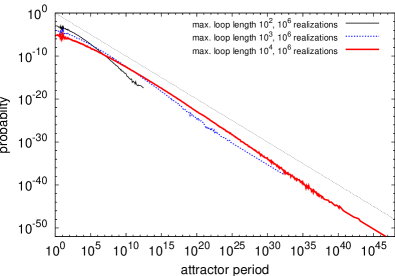
Figure 1: Distribution of attractor periods $L$. These probability distributions are found by generating relevant components and deducing the corresponding attractor period for $10^{6}$ realizations. The known loop-distribution is used, up to a cutoff value. The figure shows different cut-offs of $10^{2}$ (blue slashed line), $10^{3}$ (red crosses) and $10^{4}$ (solid black line). It is assumed that each loop contributes only to one attractor that in turn has an attractor period comparable to its number of nodes. The dotted line corresponds to a power-law with exponent $-1$. The fluctuations at small attractor periods are due to the number of divisors integers have, see text for details.

The validity of the above arguments can be explored using numerical sampling. Take $s$ different samples, each of which corresponds to a single attractor of a network realization. Note that a network realization might have more than one possible attractor, but we take only one per realization. Then, the procedure described above is implemented: Take a set of loops of length $L$, each of which occur with probability $1/L$, and calculate the ${\rm LCM}$. Using this method we end up with an histogram of attractor period, as shown in Fig. 1.

In order to display the histogram data in a logarithmic representation, the data is binned, i.e., attractor periods within a certain range are put into one bin. The width of the bins grows with a binning factor, a given bin has $b$ times the size of its neighboring bin on the left. The results are shown with a binning factor of $b=1.2$ for $L>14$, for small $L$ we just used the period of the attractor itself. By this choice we guarantee that each bin contains at least one possible attractor period. Binning is used as soon the bins may contain more than one possible attractor period, i.e., for attractors with more 14 states. The histogram is normalized such that the total probability is one. As expected, as the network size, or equivalently the maximum loop length, grows the distribution approaches a power law with exponent $-1$. Note that with this new sampling method huge system sizes can be studied. The free parameter in our method is the cutoff $L_{\rm max}$ which is a function of the system size. A further simplification is to take just the product of the individual loop periods instead of the ${\rm LCM}$.

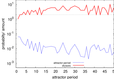
Figure 2: Probability of attractors to have period $L$ (blue dashed curve) and the number of divisors of $L$ (red solid curve). Each time the values in the upper curve have the value 2 (dotted horizontal line), $L$ is a prime number.

Consider what happens when the attractor period is short. Figure 2 shows the result using the ${\rm LCM}$ method. It also shows the number of divisors of each integer. Binning is not used in this figure. The distribution has spikes at particular periods, which are also apparent in Fig. 1. These spikes occur when the number of divisors is small. The histogram for the distribution of attractor periods in the self-organized steady state of an evolutionary Boolean network model, shown in Fig. 2 of Paczuski et al. (2000), exhibits a very similar spike-pattern. Note that in that paper, binning was used for smaller attractor periods, thus some peaks are averaged away.

As explained above, a given attractor period can be approximated by taking the least common multiple of some loop lengths (as proxy for the loop period) and we also know the probability for each loop length. If all loops up to certain length $x$ contribute to the attractor, number theory provides a formula for that. Using the prime number theorem, and an inequality proved by Nair Tenenbaum (1995), the least common multiples of the first $x$ positive integers with $x=\{1,2,\ldots\}$ obey

$$s(x) \equiv {\rm LCM}(1,2,\ldots,x)\geq\exp\left(x\left(1+\mathcal{O}(1)\right)\right)$$ (2)

The series $s(x)$ starts with $1,2,6,12,60,420,\ldots$ Sloane and Plouffe (1995) and represents all possible attractor periods. For large $x$, the probability for an attractor period constructed of all possible periods is negligible because the $e^{x}$ in Eq. (2) appears in the denominator of the probabilities for the overall attractor period. For smaller $x$, of say $x<10^{3}$, this approximation does not hold yet, but then the approximation $p(L)\sim 1/L$ does hold.

Only a full state space enumeration of the dynamics allows one to obtain the exact attractor distribution. However, this is only possible for small system sizes. This is true even if an intelligent pruning algorithm is used that disregards irrelevant nodes and simulates only the dynamics of the relevant nodes for a given realization.

For this reason, previous studies of the attractor period distribution have relied on sampling. However, sampling has potential problems Berdahl et al. (2009). One problem that can occur when generating attractor-statistics by sampling of various network realizations is undersampling. Undersampling occurs when simulating without any prior knowledge about the structure of the state space. If nothing about the relevant components is known, then one has to determine to which attractor each initial condition converges to. In order to do this, one has to determine the successor for each state, meaning $2^{N}$ updates. Because of this restriction, it is only possible to sample only a set of initial configurations that correspond to a negligible fraction of the state space for large system sizes. Another known problem that occurs with sampling is that the frequency with which attractors are found depends on the size of their basin of attraction, see e.g. Ref. Samuelsson and Troein (2003).

Our new method has neither the problem of undersampling nor of being biased by the basin sizes, and allows us to effectively study very large networks. It constructs the overall attractor of a network realization by taking the period of the relevant components the realization is constructed of. Our analytic arguments explain the numerical evidence found by others that attractor periods in large critical Boolean networks are power-law distributed. Thus, critical Boolean networks exhibit scaling also in the attractor period distribution, a property that until now has not been analytically shown.