Entanglement quantification from incomplete measurements: Applications using photon-number-resolving weak homodyne detectors

Abstract

The certificate of success for a number of important quantum information processing protocols, such as entanglement distillation, is based on the difference in the entanglement content of the quantum states before and after the protocol. In such cases, effective bounds need to be placed on the entanglement of non-local states consistent with statistics obtained from local measurements. In this work, we study numerically the ability of a novel type of homodyne detector which combines phase sensitivity and photon-number resolution to set accurate bounds on the entanglement content of two-mode quadrature squeezed states without the need for full state tomography. We show that it is possible to set tight lower bounds on the entanglement of a family of two-mode degaussified states using only a few measurements. This presents a significant improvement over the resource requirements for the experimental demonstration of continuous-variable entanglement distillation, which traditionally relies on full quantum state tomography.

1 Introduction

Entanglement is a fundamental characteristic of quantum systems and a primary resource in quantum information science. Therefore methods to experimentally measure the entanglement of the quantum state of a system are important both for the interpretation of experiments involving quantum systems and for verifying the operation and capacity of a quantum processor or communications system. The most common approach to this problem is to perform quantum tomography of the unknown state of the system [1]. Quantum state tomography amounts to measuring a tomographically complete set of observables, followed by suitably postprocessing the data. For example, in systems specified by continuous variables (such as the quadrature amplitudes of an optical field, or the position and momentum of a mechanical oscillator), the basic theoretical principle is that a collection of probability distributions of the transformed continuous variables is the Radon transform of its Wigner function. Starting from experimentally measured marginals, therefore, an inverse Radon transform gives the Wigner function from which elements of the density matrix can be obtained. The notion was first experimentally realized in the domain of quantum optics [2, 3]. Since then quantum state tomography has been improved to give controlled statistical errors using maximum-likelihood or least squares [4], made more efficient for low-rank states using ideas of compressed sensing [5], and equipped with statistical error bars [6]. This is of particular importance in the case of density matrices of non-classical states, which are typically characterized by a negative quasi-probability distribution, such as the Wigner function [7]. Reconstruction of such non-classical states is indeed a part and parcel of experimental demonstrations of quantum information protocols. Non-classical features may be difficult to reconstruct. In photonic applications, this is often due to low quantum detection efficiencies, leading to noisy measurements. [8, 9] Typically, overall detection efficiencies above $50\%$ are required. However, direct detection of other non-classical signatures may be effected using different sorts of detectors. For example, weak-field homodyne detection coupled with photon counting provides a means to detect entanglement in Gaussian states. [10, 11]

In this work we present an extensive numerical study of a strategy that provides robust direct quantative estimates for the entanglement content of a state, without the need of full quantum state tomography. In order to accomplish this task, we systematically investigate the performance of a weak-field homodyne detector with photon-number resolution as an experimentally feasible component for the construction of local measurement operators. These will be a set of positive operator valued measurements (POVMs). The POVM elements required for such a construction are characterized by a model of the homodyne detector, based on a previous characterization of the time-multiplexed photon-number-resolving detectors [12]. This detector has also been characterized using the nascent field of detector tomography [13]. The fundamental question we will answer here is the entanglement content of the least entangled state consistent with the available measurement data [14, 15, 16, 17]. Thus, we will be left with a lower bound on the entanglement of the state in question. In particular, this procedure can be used for setting a lower bound on the Logarithmic Negativity [18], the evaluation of which can be reduced to an efficiently solvable class of convex optimization problems called semidefinite programs [14, 15, 16, 17, 19]. We apply our technique to two mode photon-subtracted quadrature squeezed states. Setting bounds on such a family of non-Gaussian quantum states is of major significance for the implementation of a continuous-variable entanglement distillation protocol [20, 21].

Although we will primarily be concerned with continuous-variable entanglement distillation [21] in this work, we must make it clear at the outset that the technique studied here can be applied to any task that aims to manipulate entanglement between spatially separated observers by local operations and classical communications (LOCC), and subsequently confirm the outcome, also by means of local operations and classical communications. This goes back to the resource nature of entanglement, and the ability to manipulate it by LOCCs. Continuous variable entanglement distillation is an important instance of such a situation. It should also be clear that we are not limited to entirely optical settings, and similar techniques should be helpful to eventually identify entanglement in opto-mechanical settings, say of entanglement between a micromirror and an optical mode.

In cases such as these, it is often possible to gather enough information by a limited number of measurements to assess the correlations in the state. The natural question then is whether the correlations revealed by these local measurements (aided possibly by classical communication) represent classical correlations, or entanglement [14, 17]. This circumvents the necessity of the resource-intensive process of quantum state tomography. The method is also more robust with respect to measurement errors than full state tomography. Importantly, no a-priori assumptions concerning the purity or the specific form of the states enter the certifiable bound on the degree of entanglement.

The paper is structured as follows. In Sec. (2), we formalize as a semidefinite program (SDP) the problem of putting lowers bounds on the entanglement content of states using localized measurement statistics. Sec. (3) describes the specific time-multiplexed homodyne detector that we use to build these localized measurements. In Sec. (4), we present the numerical results on the bounds set on the entanglement content of a two-mode photon subtracted quadrature squeezed state, for different values of relevant experimental parameters. We also present an extensive numerical exploration of the performance of the detector under different experimental conditions. In particular, we analyze the required phase accuracy and phase stability in our homodyne scheme. We also discuss the tolerance of the convex optimization algorithm to experimental noise. Finally, in Sec. (5) we report the conclusions. As a matter of notation, all logarithms in this paper are taken to base $2$.

2 Lower bounds using convex optimization

As stated in the introduction, we are seeking the amount of entanglement in the least entangled state compatible with a set of measurement results. Mathematically, this can be presented as

$$E_{\min}=\min_{\rho}\{E(\rho):\mathrm{Tr}(\rho M_{i})=m_{i}\},$$ (1)

where $E$ is the measure of entanglement, and $M_{i}$ are the measurements made with measurement data $m_{i}.$ Additional constraints that $\rho$ is a density matrix, i.e., positive, and $\mathrm{Tr}(\rho)=1$, are also imposed. The latter is easily done by setting $M_{0}=\mathbb{I}$ and $m_{0}=1.$ Depending on the measure of entanglement, and the measurements chosen, the minimization in Eq. (15) can even be performed analytically, but generically that is not the case. Here, we briefly present a technique following the presentation in Refs. [14, 15] that allows the above problem to be cast as a semidefinite program when the entanglement measure is the Logarithmic Negativity [18].

Logarithmic Negativity is defined as the logarithm of the 1-norm of the partial transposed density matrix $\|\rho^{T_{1}}\|_{1}.$ The 1-norm can be expressed as [22]

$$\|\rho^{T_{1}}\|_{1}=\max_{\|H\|_{\infty}=1}\mathrm{Tr}(H\rho^{T_{1}})=\max_{\|H\|_{\infty}=1}\mathrm{Tr}(H^{T_{1}}\rho),$$ (2)

with the maximization being over all hermitian operators $H$, where $\|.\|_{\infty}$ denotes the standard matrix operator norm, namely the largest singular value of the matrix. Using the monotonicity of the logarithm, the minimization in Eq. (15) can be rewritten as

$$\mathcal{N}_{\min}=\log\min_{\rho}\left\{\max_{H}\{\mathrm{Tr}(H^{T_{1}}\rho)\big{|}\|H\|_{\infty}=1\}:\mathrm{Tr}(\rho M_{i})=m_{i}\right\}.$$ (3)

The minimax equality allows us to interchange the maximization and the minimization, leading to

$$\mathcal{N}_{\min}=\log\max_{H}\left\{\min_{\rho}\{\mathrm{Tr}(H^{T_{1}}\rho):\mathrm{Tr}(\rho M_{i})=m_{i}\}:\|H\|_{\infty}=1\right\}.$$ (4)

For any real numbers $\{\nu_{i}\}$ for which

$$H^{T_{1}}\geq\sum_{i}\nu_{i}M_{i},$$ (5)

clearly the lower bound

$$\mathrm{Tr}(H^{T_{1}}\rho)\geq\sum_{i}\nu_{i}\mathrm{Tr}(M_{i}\rho)=\sum_{i}\nu_{i}m_{i}.$$ (6)

holds true for states $\rho$. Thus we get

$$\mathcal{N}_{\min}\geq\log\max_{H}\left\{\max_{\nu_{i}}\big{\{}\sum_{i}\nu_{i}m_{i}:H^{T_{1}}\geq\sum_{i}\nu_{i}M_{i}\big{\}}:\|H\|_{\infty}=1\right\}.$$ (7)

Note that the state $\rho$ drops completely out of contention now. Since the inner minimization in Eq. (4) is a semidefinite program, strong duality in the strictly feasible case ensures equality in Eq. (7). Thus, having fixed the operators that we choose to measure $M_{i},$ any choice of $H$ and $\nu_{i}$ such that $H^{T_{1}}\geq\sum_{i}\nu_{i}M_{i}$ and $\|H\|_{\infty}=1,$ provides us with a lower bound on the Logarithmic Negativity of states which provide expectation values of $m_{i}.$ Finally, we can rewrite Eq. (7) as

$$\mathrm{maximize}\;\;\;\log\Big{(}\sum_{i}\nu_{i}m_{i}\Big{)},$$ (8)

$$\mathrm{subject\;to}\;\;H^{T_{1}}\geq\sum_{i}\nu_{i}M_{i},$$

$$\;\;\;\;\;\;\mathrm{and}\;\;\;-\mathbb{I}\leq H\leq\mathbb{I},$$

which can be solved quite easily using standard SDP solvers, like SeDuMi [23], once we have decided what our measurements $M_{i}$ are. Since these are to be local, the typical form of the measurement, in the case of bipartite states, is

$$M_{i}=\Pi^{1}_{j}\otimes\Pi^{2}_{k}.$$ (9)

The problem is thus reduced to the construction of the operators $\Pi^{1,2}_{j},$ which is what we move onto in the next section. In passing, we mention that the choice of these measurement operators can also be cast as a SDP, although it is more challenging to incorporate the locality constraint into its framework.

This idea gives useful and practically tight bounds to the entanglement content, not having to assume any a-priori knowledge about the state, or properties of it such as its purity. If the set of expectation values $\{\mathrm{Tr}(M_{i}\rho)\}$ is tomographically complete, obviously, the bound is promised to give the exact value, but in practice, a much smaller number of measurements is sufficient to arrive at good bounds. Data of expectation values can be composed, that is if two sets of expectation values are combined, the resulting bound can only become better, to the extent that two sets that only give rise to trivial bounds can provide tight bounds. The approach presented here is perfectly suitable for any finite-dimensional system, and also for continuous-variable systems, as long as the observables $M_{i}$ are bounded operators. Photon counting with a phase reference gives rise to such operators, as we will see. Note also that similar ideas, formulating lower bounds to entanglement measures, constraining expectation values of observables can also be formulated for other measures of entanglement [15, 16]. This is in line with the idea of systems identification of trying to directly estimate relevant quantities, instead of aiming at the detour of reconstructing the quantum states first.

3 Photon-number-resolved weak homodyne detection

We consider now the application of entanglement quantification to detection of entangled photonic states. In this application we propose to make use of photon-number resolving detectors. These have several useful features that make them well-suited to the measurement of non-classical signatures of light beams. First, weak-field homodyne detection provides a way to demonstrate the entangled character of EPR-like two-mode squeezed states [10, 11, 24], in contrast to strong-field homodyne detection [25]. Second, because the amplitude of the local oscillator is comparable to that of the signal, the phase sensitivity of the photon counting distribution is much smaller than that of a regular homodyne detector. This greatly reduces the problem of synchronizing local reference frames, which generally becomes more difficult with increasing distance.

Within the framework of the quantum theory of measurement, the action of a detector is completely specified by its positive operator valued measurement (POVM) set [26]. A POVM element is a positive definite operator $\Pi_{\beta,\gamma}\geq 0$, which represents the outcome $\beta$ of a given detector, for a setting $\gamma$ corresponding to a particular value for a tunable parameter in the detector. In the case of a homodyne detector, $\gamma$ would correspond to the phase or the amplitude of the local oscillator. The complete set should satisfy $\sum_{\beta}\Pi_{\beta,\gamma}=\mathbb{I}$. The probability $p_{\beta,\gamma}$ of obtaining outcome $\beta$ for setting $\gamma$ can be related to the state of the system $\rho$ by $p_{\beta,\gamma}=\mathrm{Tr}(\rho\Pi_{\beta,\gamma})$.

Our detection scheme consists of a weak local oscillator (LO) mixed with the signal $\rho$ at a variable reflectivity ($R$) beam-splitter (BS). The outcome of such an interference is collected by time-multiplexed photon-number-resolving (PNR) detectors [27]. The time-multiplexed detectors (TMD) split the incoming pulses into $8$ distinct modes, which are eventually detected by binary avalanche photo-diodes (APDs) which can register either $0$ or $1$ click. Thus there are $9$ possible outcomes for a given TMD which are labelled by the number of clicks $\beta=0,\dots,8$. The settings of the detector $\gamma$, in turn, are determined by a number of experimental parameters, such as LO amplitude $|\alpha|$ and phase $\theta$, BS reflectivity $R$, and detector efficiency $\eta$. By tuning the detector settings it is possible to prepare POVM elements able to project onto a large variety of radiation field states, ranging from Fock states to quadrature squeezed states [12].

3.1 Detector model

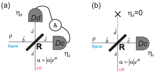
Figure 1: Homodyne detection scheme for (a) balanced and (b) unbalanced configuration. $D_{c,d}$ are PNR detectors of the time-multiplexed type.

In Fig. (1 (a)) we show a schematic of our detection system for the balanced configuration. The BS input modes, labeled $a$ and $b$, correspond to the LO and the signal ($\rho$), respectively. The output modes, labeled by $c$ and $d$, are detected by PNR detectors $D_{c}$ and $D_{d}$. The joint detection events, denoted $\{\beta=(n_{c},n_{d})\}$, are recorded for different LO settings $\gamma=(|\alpha|,\theta)$. The LO, is prepared in a coherent state with state vector $|\alpha\rangle$ of complex amplitude $\alpha=|\alpha|e^{i\theta}$ and provides the phase reference needed to access off-diagonal elements in $\rho$, as the PNR detectors alone have no phase sensitivity [27]. For ideal PNR detectors, the probability to obtain measurement outcome $\beta$ for LO setting $\gamma$ is related to $\rho$ by [28]

$$p_{\beta,\gamma}=\mathrm{Tr}_{c,d}[{U}\sigma{U}^{\dagger}|n_{c},n_{d}\rangle\langle n_{c},n_{d}|],$$ (10)

where $U=e^{i\chi(b^{\dagger}a+a^{\dagger}b)}$ is the unitary operator representing the BS, $R=\cos(\chi)^{2}$ is the BS reflectivity, $\sigma=|\alpha\rangle\langle\alpha|_{a}\otimes\rho_{b}$ the two-mode input state and $|n_{c},n_{d}\rangle=|n_{c}\rangle_{c}|n_{d}\rangle_{d}$ the photon number state vectors of mode $c$ ($d$) to be detected at PNR detectors $D_{c}$ ($D_{d}$).

In order to account for the imperfections of the time-multiplexed PNR detectors we use a well tested model of the TMDs [27]. Within this model, the TMD operation can be described as a map from the incoming photon-number distribution $\vec{r}$, as a vector (i.e., the diagonal components of the density matrix) to the measured click statistics $\vec{k}$ by $\vec{k}=C\cdot L\cdot\vec{r}$. Here $L$ and $C$ are matrices accounting for loss and the intrinsic detector structure [27], respectively. To calculate the POVM elements implemented by our PNR homodyne detector, the POVMs for TMD detectors $D_{c}$ and $D_{d}$ are determined from the $C$ and $L$ matrices (characterized by independent methods [13]). The TMD POVMs are then substituted into Eq. (10), in place of the photon number projectors $|n_{c},n_{d}\rangle\langle n_{c},n_{d}|$, to obtain the final expression for the imperfect POVM elements $\Pi_{\beta,\gamma}$. We note that our TMDs can resolve up to $8$ photons, setting the number of possible outcomes to $81$.

3.2 Unbalanced detection scheme

Our aim is to use such homodyne PNR detectors to provide lower bounds on the entanglement of bipartite quantum states, in which case two of such devices should be employed. To this end, the joint POVM statistics of the four modes involved in the detection need to be measured, increasing the total number of POVM elements to $81^{2}=6561.$ In order to simplify the experimental arrangement, we use the detector in an unbalanced configuration, so that we only detect one of the outgoing modes of each homodyne BS. In this way only two modes need to be jointly detected and the total number of POVM elements is reduced to $9^{2}=81$. This unbalanced scheme can be modeled by setting the efficiency $\eta$ of one the PNR detectors to zero (see Fig. (1 (b))). The only disadvantage of this unbalanced scheme is that the overall efficiency is in principle reduced by $50\%$, but this limitation can be overcome by increasing the BS reflectivity $R$. Additionally, as we will show in the next section, our partial detection approach alleviates the strong efficiency requirements of full tomography allowing for the additional losses of the unbalanced scheme.

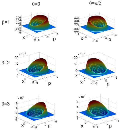
Figure 2: Wigner representation of selected POVM elements $\Pi_{\beta,\gamma}$ for the unbalanced scheme described in Fig. (1 (b)). Different columns correspond to LO phase settings $\theta=0$ and $\theta=\pi/2$. The rows correspond to three different detector outcomes $\beta=1,2,3$. The amplitude of the LO, BS reflectivity and detector efficiency are, $|\alpha|=1$, $R=50\%$ and $\eta=10\%$ , respectively.

In Fig. (2), we show numerically constructed Wigner functions corresponding to $6$ different POVM elements $\Pi_{\beta,\gamma}$, characterizing the unbalanced scheme. The axes $(x,p)$ label the phase space quadratures. The different columns correspond to different LO phases $\theta=0$ and $\theta=\pi/2$. The rows correspond to three consecutive outcomes $\beta=1,2,3$, labelling the corresponding number of detector clicks. For these simulations we fixed the amplitude of the LO to $|\alpha|=1$, the BS reflectivity to $R=50\%$ and the detector efficiency to $\eta=10\%$, which is a realistic value for a single mode TMD. The figure shows that $\Pi_{\beta,\gamma}$ are not rotationally symmetric, as expected for a phase sensitive detector. The oscillations in the Wigner functions are due to the low efficiency of the detectors which mixes different photon number states, whose phase-space representation is given by consecutive rings of increasing radii. Also, as is expected, a change in the LO phase setting by $\pi/2$ corresponds to an overall phase-space rotation in the Winger function. In the next section we show that by using $8$ POVM elements of the type shown in Fig. (2) for each subsystem, we can construct the measurements $M_{i}$ mentioned in Sec. (2), which can be employed to bound the entanglement content of two-mode degaussified states.

4 Application to continuous-variable entanglement distillation

We will now apply the above methods to a setting that plays a central role in continuous-variable entanglement distillation. Entanglement distillation aims at producing more highly entangled states out of a situation where entanglement is present only in a dilute and noisy form, presumably generated by some lossy quantum channel. It provides the key step in quantum repeater ideas allowing for the distribution of long-range entanglement in the presence of noise. Crudely speaking, one may distinguish between actual distillation schemes that involve more than one specimen of an entangled state at each step of the protocol, and “Procrustean” or local filtering approaches that take a single copy of a state and under appropriate local filtering give rise – if successful – to a more highly entangled state. In the setting of strict Gaussian operations, continuous-variable entanglement distillation of neither kind is possible [21], but this obstacle can be overcome with the help of non-Gaussian ingredients such as photon addition or subtraction [20]. Such first Procrustean steps can also be used as starting points in full entanglement distillation protocols. Indeed, quite exciting first steps towards full continuous-variable entanglement distillation have recently been taken experimentally [9, 30, 31, 32, 33].

In the subsequent discussion we show the use of quantitative tests to certify success in such a scheme. Needless to say, we discuss specific input states, but it should be clear that the given entanglement bounds do not make use of that a-priori knowledge. We consider as our initial state vector $|\psi^{\mathrm{ini}}\rangle$ an ideal pure two-mode quadrature squeezed state of the form

$$|\psi^{\mathrm{ini}}\rangle=\sqrt{1-\lambda^{2}}\sum_{n=0}^{\infty}\lambda^{n}|n,n\rangle_{1,2},$$ (11)

where $\lambda$ represents the squeezing parameter, and the subindices $(1,2)$ represent each spatial mode. Such type of states are produced in the laboratory by the non-linear process of spontaneous parametric down conversion (SPDC) in non-linear crystals [29]. In order to simplify our numerical calculations, we will restrict the maximum photon-number per mode to $n_{\mathrm{max}}=3$. Thus the set of bipartite initial states $\rho_{1,2}^{\mathrm{ini}}$ is given by the set of $16\times 16$ density matrices $\rho_{1,2}^{\mathrm{ini}}=|\psi^{\mathrm{ini}}\rangle\langle\psi^{\mathrm{ini}}|$. The Logarithmic Negativity for the bipartite state in Eq. (11) takes the simple form

$$\mathcal{N}(\rho_{1,2}^{\mathrm{ini}})=\log\|(\rho_{1,2}^{\mathrm{ini}})^{T_{1}}\|_{1}=\log\left(\frac{1+\lambda}{1-\lambda}\right),$$ (12)

as can readily be verified.

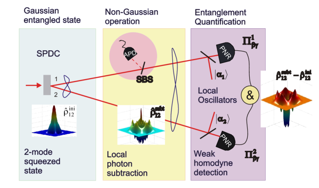
Figure 3: (Color online) Scheme describing the bipartite initial state $\rho_{1,2}^{\mathrm{ini}}$ produced by spontaneous parameteric down conversion (SPDC). Next, the poton-subtracted state $\rho_{1,2}^{\mathrm{subt}}$ is prepared by local subtraction of a single photon at a tunable subtraction beam splitter (SBS). The entanglement content in $\rho_{1,2}^{\mathrm{subt}}$ is quantified by our partial detection approach. This type of scheme is one of the main components of an entanglement distillation protocol [20].

4.1 Two-mode photon-subtracted quadrature squeezed state

In order to distill continuous-variable entanglement from Gaussian states, such as the two-mode quadrature squeezed state described by Eq. (11), an operation that removes the Gaussian nature of the probability distribution is required [20]. Examples of such non-Gaussian operations are the conditional subtraction or addition of a photon [9, 33]. An ideal two-mode photon-subtracted quadrature squeezed state can be modeled by inserting a BS of transmission $T$ (the so-called subtraction beam-splitter SBS) in one spatial mode. The reflected mode from the SBS is then detected by a standard (ideal) avalanche photodetector (APD) (this is schematized in Fig. (3)). The photon subtracted state can, in the approximation of having a a very weakly reflecting beam-splitter, thus be written as

$$|\psi^{\mathrm{subt}}\rangle=C\sum_{n=1}^{n_{\max}}(\lambda T)^{n}\sqrt{n}|n-1,n\rangle_{1,2},$$ (13)

where $C$ is a normalization constant and in our simulations $n_{\mathrm{max}}=3$. The corresponding density matrix is $\rho_{1,2}^{\mathrm{subt}}=|\psi^{\mathrm{subt}}\rangle\langle\psi^{\mathrm{subt}}|$. We note that the family of states described by Eq. (13) are of current interest in the realm of continuous-variable entanglement distillation, as they represent a particular kind of non-Gaussian state (i.e., a state whose Wigner representation is not Gaussian), whose entanglement content $\mathcal{N}(\rho^{\mathrm{subt}}_{1,2})$ is predicted to be larger than $\mathcal{N}(\rho^{\mathrm{ini}}_{1,2})$, for suitable experimental parameters ($\lambda$, $T$) [21].

4.2 Construction of the observables

Our aim is to construct bipartite measurement operators $M_{i}$ as a tensor product of the POVM elements corresponding to each subsystem $\Pi_{1}\otimes\Pi_{2}$. In particular, we will consider $8$ POVM elements for each subsystem $(1,2)$, specified by four different outcomes $\beta=0,1,2,3$ and two different settings $\gamma$ corresponding to $\theta=0$ and $\theta=\pi/2$. Thus the selected POVM subset for each mode consist of $8$ elements $\Pi_{\beta,\gamma}$, collected as

$$\{\Pi_{0,0},\Pi_{1,0},\Pi_{2,0},\Pi_{3,0},\Pi_{0,\pi/2},\Pi_{1,\pi/2},\Pi_{2,\pi/2},\Pi_{3,\pi/2}\},$$ (14)

where we will keep this ordering in the POVM elements for the rest of the paper. We measure $8\times 8$ configurations, which determine $64$ POVMs $M_{i}$, labelled by the index $i$, of the form in Eq. (9) with $j,k=1,\dots,8$ being the indices labelling the POVM elements of mode $(1,2)$ respectively, and $i=(j,k)$ the joint index, labelling the bipartite measurement operator. For example, the observable $M_{(6,1)}$ corresponds to the POVM elements $\Pi_{1,\pi/2}$ for mode 1 and $\Pi_{0,0}$ for mode $2$. This gives a total of 64 measurements, which in turn determine 64 expectation values $\mathrm{Tr}(\rho_{1,2}M_{i})=m_{i}$, with $i=1,\dots,64$. This is a clear reduction with respect to full state tomography, which would require (at least) $16^{2}-1=255$ measurements in order to reconstruct $\rho_{1,2}$ in a truncated Hilbert space of dimension $16$.

In order to find the lower bound on the Logarithmic Negativity of the photon-subtracted states $\rho_{1,2}^{\mathrm{subt}}$ described in Eq. (13), by means of the set of measurement observables $M_{i}$ as defined in Eq. (9), we follow the procedure described in Sec. (2). Note that in a real experiment $\mathrm{Tr}(\rho_{1,2}^{\mathrm{subt}}M_{i})$ should be replaced by the actual experimental probability estimates which will be subject to different sources of noise. We will discuss the effect of experimental noise on entanglement bounds in the final subsection.

4.3 Numerical results

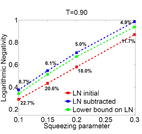
Figure 4: (Color online) Logarithmic Negativity (LN) for the initial state (red curve), subtracted state (blue curve) and lower bound on LN of subtracted state obtained by convex optimization (green curve), vs. squeezing parameter ($\lambda$). Percentual entanglement increase with a single photon-subtraction step and percentual difference between the actual LN of the subtracted state and the one obtained by convex optimization are indicated. The SBS transmission was fixed at $T=90\%$.

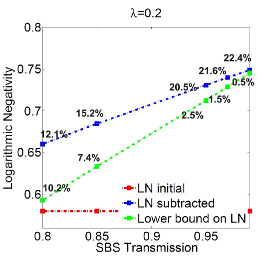
Figure 5: (Color online) Logarithmic Negativity (LN) for the initial state (red curve), subtracted state (blue curve) and lower bound on LN of subtracted state obtained by convex optimization (green curve), vs. SBS transmission ($T$). Percentual entanglement increase with a single photon-subtraction step and percentual difference between the actual LN of the subtracted state and the one obtained by convex optimization are indicated. The squeezing parameter was fixed at $\lambda=0.2$.

Fig. (4) presents the percentual entanglement increase between $|\psi^{\mathrm{ini}}\rangle$ (red curve) and $|\psi^{\mathrm{subt}}\rangle$ (blue curve) for different squeezing parameters $\lambda$ ranging from $\lambda=0.1$ to $\lambda=0.3$. Percentual differences between the actual Logarithmic Negativity characterizing the photon-subtracted state and the lower bound obtained by convex optimization (green curve) are also indicated. The transmission coefficient of the subtraction beam-splitter (SBS) in Fig. (2) was fixed at ($T=90\%$), the LO amplitude and detector efficiency were set to $|\alpha|=1$ and $\eta=10\%$, respectively. It is noticeable that while a single-photon-subtraction step produces a larger entanglement increase for lower values of $\lambda$, the lower bound on the entanglement becomes tighter for higher squeezing parameter $\lambda$. The percentual error in the lower bound is in all cases below $9\%$, which reveals the accuracy of our partial detection scheme in characterizing entanglement.

Fig. (5) presents the percentual entanglement increase between $|\psi^{\mathrm{ini}}\rangle$ (red curve) and $|\psi^{\mathrm{subt}}\rangle$ (blue curve) for different SBS transmission $T$, ranging from $T=80\%$ to $T=99\%$. Percentual differences between the actual Logarithmic Negativity characterizing the photon-subtracted state vector ($|\psi^{\mathrm{subt}}\rangle$) and the lower bound obtained by convex optimization (green curve) are also indicated. The squeezing parameter was fixed at ($\lambda=0.2$), the LO amplitude and detector efficiency were set to $|\alpha|=1$ and $\eta=10\%$, respectively. Fig. (5) shows that for a fixed squeezing parameter the single-photon-subtraction step produces a larger entanglement increase for higher SBS transmission $T$ and that the lower bound becomes tighter for higher $T$. In all cases, the percentual error in the lower bound remains below $11\%$.

Next, we tested the robustness of the measurement scheme with respect to different types of LO phase noise. To this end we constructed a set of 64 POVM elements as described in the previous section, for a fixed LO amplitude $\alpha=1$, detector efficiency $\eta=0.10$, SBS transmission $T=0.90$ and squeezing parameter $\lambda=0.2$. The two fixed phase setting $\theta_{0}=(0,\pi/2)$ were subject to different types of fluctuations. In particular, we investigated the required precision in the LO phase $\theta$ by adding different amounts of random phase noise $\epsilon$ in the form $\theta=(0\pm\epsilon/10,\pi/2(1\pm\epsilon/10))$, where $0\leq\epsilon\leq 1$ is a random number with a uniform distribution. In our numerical simulations we found that for a phase error of up to $10\%,$ the lower bound differs from the actual Logarithmic Negativity by less than $1\%$. This means that an LO phase precision of 5 degrees (at the most) is required for the bounds to produce a highly tight estimate. This is shown in Fig. (6 (a)), for $\theta_{0}=(0,\pi/2)$, a squeezing parameter $\lambda=0.2$, a SBS transmission $T=90\%$, an LO amplitude $|\alpha|=1$ and a detector efficiency $\eta=0.10$.

We also analyzed the effect of temporal phase fluctuations, by modelling the LO as a phase averaged coherent state described by the complex amplitude $\alpha=\sum_{j}|\alpha|e^{i(\theta_{0}+\delta\theta_{j})}$ with $j=1,\dots,100$ and $\delta\theta$ a random phase with a uniform distribution centered around $\theta_{0}\in[0,\pi/2]$ and with width $\Delta\theta$. We found that a phase width of up to $0.6$ radians ($\approx 30$ degrees) introduces a percentual difference in the lower bound of up to $15\%$. For a phase width $\Delta\theta$ of up to $0.4$ radians ($\approx 20$ degrees) the lower bound on the logarithmic negativity is within $10\%$. This is shown in Fig. (6 (b)), for a squeezing parameter $\lambda=0.2$, a SBS transmission $T=90\%$, an LO amplitude $|\alpha|=1$ and a detector efficiency $\eta=0.10$.

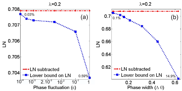
Figure 6: (Color online) Exact Logarithmic Negativity (red curve) and lower bound obtained by convex optimization (blue curve) for the photon-subtracted state vs. (a) dimensionless phase noise $\epsilon$ and (b) phase noise standard deviation $\Delta\theta$ in radians for LO phase settings $\theta_{0}=(0,\pi/2)$. Max. and min. percentual differences are indicated. The squeezing parameter was fixed at $\lambda=0.2$.

Finally, we analyzed the impact of a different homodyne BS reflectivity $R$ on the overall accuracy of the entanglement quantification scheme. We found that for $R\geq 80\%$ the lower bound on the Logarithmic Negativity differs by less than $0.2\%$ from the actual value, as long as the LO amplitude remains small enough ($|\alpha|\leq 2.5$) due to the limited photon-number resolution in the time-multiplexed detectors. This is shown in Fig. (7 (a)). Fig. (7 (b)) shows a complete simulation for $50\%\leq R\leq 99\%$, $|\alpha|=2.5$, $\lambda=0.1$ and $T=90\%$. In all the simulations, the TMD efficiencies were set to $\eta=0.10$ and the LO phase settings were chosen as $\theta=(0,\pi/2)$. Additionally, the subtraction APD in Fig. (3) is assumed to have a limited efficiency, which is modelled by interposing a beamsplitter with transmittivity of $15\%$. The numerical simulations in this work were implemented using the convex optimization package SeDuMi [23].

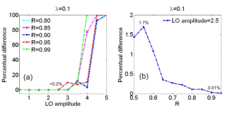
Figure 7: (Color online) (a) Percentual error in the lower bound set by convex optimization for different homodyne BS reflectivities $R$. The error remains below $0.2\%$ for a sufficiently weak LO amplitude $|\alpha|<2.5$. (b) Extension to a larger range of BS reflectivities $R$, for $\lambda=0.1$, $|\alpha|=2.5$, $\theta=(0,\pi/2)$.

4.4 Tolerance to experimental measurement errors

In the numerical simulations presented here we have used the exact expectation values $m_{i}=\mathrm{Tr}(\rho^{\mathrm{subt}}M_{i})$ for the minimization of Logarithmic Negativity. However, in a real experiment such expectation values are affected by different sources of noise. In this subsection, we test the tolerance of the scheme to experimental errors. There are several ways to include such an error. One approach would be to estimate variances of measured values, and then make a model including Gaussian-distributed errors for the measured variables. Another would be a hard bound on the degree of entanglement as a function of a small norm deviation from the perfect data, giving rise to a box error model. This latter error model even allows for a malicious correlation in the errors, in that all errors add constructively. Clearly, independent, identically distributed errors would give rise to much more robust bounds.

Nonetheless, in order to evaluate the feasible robustness of our method, we will now refer to this latter, more demanding error model: We merely require for an $\epsilon>0$ that the measured value $n_{i}$ and the true expectation value $m_{i}=\mathrm{Tr}{(M_{i}\rho)}$ satisfy $m_{i}\in[(1-\epsilon)n_{i},(1+\epsilon)n_{i}]$ for all $i$. Hence, the problem to be solved becomes

$$\mathcal{N}_{\min}=\min_{\rho}\{\mathcal{N}(\rho):\mathrm{Tr}(\rho M_{i})=n_{i},\,m_{i}\in[(1-\epsilon)n_{i},(1+\epsilon)n_{i}]\,\,\,\forall i\},$$ (15)

Including such measurement errors, Eq. (8) then clearly becomes

$$\mathrm{maximize}\;\;\;\;\log\Big{(}\sum_{i}\nu_{i}n_{i}\Big{)},$$ (16)

$$\mathrm{subject\;to}\;\;H^{T_{1}}\geq\sum_{i}\nu_{i}M_{i},$$

$$\hskip 56.9055ptm_{i}\in[(1-\epsilon)n_{i},(1+\epsilon)n_{i}]\,\,\forall i,$$

$$\;\;\;\;\;\;\mathrm{and}\;\;\;-\mathbb{I}\leq H\leq\mathbb{I},$$

which can be solved as easily as Eq. (8) using SeDuMi [23]. Note that the resulting bound is even valid if each of the errors in the measured data are maliciously correlated.

In this subsection, we use as an example a two-mode squeezed state with $\lambda=0.2$ from which a photon is subtracted using a SBS with $T=95\%.$ The APD in Fig. (2) is assumed to have a limited efficiency, which is achieved by interposing a beamsplitter with transmittivity of $20\%.$ In a short table below, we present the bounds attained by solving the SDP in Eq. (16) for some representative values of $\epsilon.$

$\epsilon$	0.0	0.001	0.01	0.1
$\mathcal{N}_{\min}$	0.7308	0.7185	0.6660	0.3034

These numbers must be compared with the entanglement of the initial two-mode squeezed state, which has $\mathcal{N}=0.5803,$ and the ideal photon subtracted state which has $\mathcal{N}=0.7309.$ Note that the state on which we put the lower bounds is inevitably mixed, and the table shows the robustness and effectiveness of our scheme. $\epsilon=0.01$ is enough to demonstrate the enhancement of entanglement by distillation with experimentally realistic parameters, without having to undertake a full tomography of the quantum states involved. This value of $\epsilon$ translates to about $10000$ data points, via the central limit theorem, for each measurement configuration. This is in line with the number of data points taken in other experiments involving reconstruction of non-Gaussian states [9].

5 Conclusions

We have presented quantitative numerical evidence that a novel homodyne detection scheme with photon-number resolution is able to set accurate bounds on the entanglement content of a family of two-mode photon-subtracted quadrature squeezed states. The entanglement lower bounds retrieved by the measurement scheme are accurate to within $10\%$ for the full range of squeezing parameters $\lambda=0.1-0.3$ and subtraction beam-splitter transmissions $T=80\%-99\%$. We found that the bounds become tighter for higher $\lambda$ and $T$. We also analyzed the required phase precision and stability in the local oscillator (LO), and found that a precision of less than $5$ degrees is required for a bound accuracy within $1\%$, while temporal phase fluctuations of up to $20$ degrees can be accepted for a lower bound with $10\%$ accuracy. Additionally we found that a homodyne beam-splitter reflectivity $R$ above $60\%$, for an LO amplitude within $|\alpha|=2.5$ is sufficient to obtain a lower bound on the Logarithmic Negativity which agrees to within $2\%$ with the actual Logarithmic Negativity value characterizing the photon-subtracted state. The results reported here provide strong numerical evidence of the suitability of our partial detection scheme for entanglement quantification of bipartite degaussified states. We note that this type of partial detection approach is not only attractive due to its accuracy but also due to its scalability. This is of importance for the application of an entanglement distillation protocol combining two degaussified sources [20, 21]. In particular, our scheme can be easily scaled to the detection of four spatial modes, in which case it would require the measurement of only $64^{2}=4096$ outcome probabilities. In contrast, full state tomography would require (at least) $16^{4}-1=65535$ different measurements. Therefore our method provides a feasible, direct and resilient way of accurately experimentally characterizing entanglement in continuous-variable quantum systems. Finally, we anticipate the amount of data required in order to obtain an adequate precision in the measurement-outcome probabilities characterizing our partial measurement scheme to be considerably lower than that required for full state tomography.

References

References

- [1] G. M. D’Ariano, M. G. A. Paris, and M. F. Sacchi, Advances in Imaging and Electron Physics 128, 205 (2003).
- [2] D. Smithey, M. Beck and M. Raymer, and A. Faridani, Phys. Rev. Lett. 70, 1244 (1993).
- [3] T. Dunn, I. A. Walmsley and S. Mukamel, Phys. Rev. Lett. 74, 884 (1995).
- [4] M. P. A. Branderhorst, I. A. Walmsley, R. L. Kosut, and H Rabitz, J. Phys. B 41, 074004 (2008); R. L. Kosut, I. A. Walmsley, and H. Rabitz, arXiv quant-ph/0411093 (2004).
- [5] D. Gross, Y.-K. Liu, S. Flammia, S. Becker, and J. Eisert, arxiv:0909.3304 R.L. Kosut, arXiv:0812.4323; A. Shabani, R.L. Kosut, and H. Rabitz, arXiv:0910.5498.
- [6] K. M. R. Audenaert and S. Scheel, New J. Phys. 11, 023028 (2009).
- [7] M. Hillery, R. F. O’Connell, M. O. Scully, and E. P. Wigner, Phys. Rep. 106, 121 (1984); W. P. Schleich, Quantum optics in phase space, Wiley, Berlin (2001).
- [8] A. I. Lvovsky and M. G. Raymer, Rev. Mod. Phys. 81, 299 (2009).
- [9] A. Ourjoumtsev, A. Dantan, R. Tualle-Brouri, and P. Grangier, Phys. Rev. Lett. 98, 030502 (2007).
- [10] P. Grangier, M. J. Potasek and B. Yurke, Phys. Rev. A, 38, R3132 (1988).
- [11] A. Kuzmich, I. A. Walmsley, and L. Mandel, Phys. Rev. Lett., 85, 1349 (2000).
- [12] G. Puentes, J. S. Lundeen, M. P. A. Branderhorst, H. B. Coldenstrodt-Ronge, B. J. Smith, and I. A. Walmsley, Phys. Rev. Lett. 102, 080404 (2009).
- [13] J. S. Lundeen, A. Feito, H. Coldenstrodt-Ronge, K. L. Pregnell, Ch. Silberhorn, T. C. Ralph, J. Eisert, M. B. Plenio, and I. A. Walmsley, Nature Physics, 5, 27 (2009); A. Feito, J. S. Lundeen, H. Coldenstrodt-Ronge, J. Eisert, M. B. Plenio, and I. A. Walmsley, New J. Phys. 11, 093038 (2009); H.B. Coldenstrodt-Ronge, J. S. Lundeen, A. Feito, B.J. Smith, W. Mauerer, Ch. Silberhorn, J. Eisert, M. B. Plenio, I.A. Walmsley, J. Mod. Opt. 56, 432 (2009).
- [14] K. M. R. Audenaert and M. B. Plenio, New J. Phys. 8, 266 (2006).
- [15] J. Eisert, F. G. S. L. Brandão, and K. M. R. Audenaert, New J. Phys. 8, 46 (2007).
- [16] O. Gühne, M. Reimpell, and R. F. Werner, Phys. Rev. Lett. 98, 110502 (2007).
- [17] M. B. Plenio, Science, 324, 342 (2009).
- [18] M. B. Plenio, Phys. Rev. Lett. 95, 090503 (2005); J. Eisert, PhD thesis (Potsdam, February 2001); G. Vidal and R.F. Werner, Phys. Rev. A 65, 032314 (2002).
- [19] S. Boyd and L. Vandenberghe, Convex optimization, Cambridge University Press, Cambridge (2005).
- [20] D. E. Browne, J. Eisert, S. Scheel, and M. B. Plenio, Phys. Rev. A 67, 062320 (2003); J. Eisert, D. E. Browne, S. Scheel, and M. B. Plenio, Annals of Physics (NY) 311, 431 (2004).
- [21] J. Eisert, S. Scheel, and M. B. Plenio, Phys. Rev. Lett. 89, 137903 (2002); J. Fiurasek, Phys. Rev. Lett. 89, 137904 (2002); G. Giedke and J. I. Cirac, Phys. Rev. A 66, 032316 (2002).
- [22] R. Bhatia, Matrix analysis, Springer, New York (1997).
- [23] All the simulations in this work were preformed using the convex optimization routine SeDuMi 1.1, available for free downloading at http://sedumi.ie.lehigh.edu.
- [24] K. Banaszek and K. Wodkiewicz, Phys. Rev. A 58, 4345 (1998); Phys. Rev. Lett. 98 82, 2009 (1999).
- [25] Z. Y. Ou, S. F. Pereira, H. J. Kimble, and K. C. Peng, Phys. Rev. Lett., 68, 3663 (1992).
- [26] A. S. Holevo, Probabilistic and statistical aspects of quantum theory, North Holland, Amsterdam (1982).
- [27] D. Achilles, C. Silberhorn, C. Sliwa, K. Banaszek, I. A. Walmsley, M. J. Fitch, B. C. Jacobs, T. B. Pittman, and J.D. Franson, J. Mod. Opt. 51, 1499 (2004).
- [28] K. L. Pregnell, and D. T. Pegg, Phys. Rev. A 66, 013810 (2002).
- [29] P. J. Mosley, J. S. Lundeen, B. J. Smith, P. Wasylczyk, A. B. U’Ren, Ch. Silberhorn, and I. A. Walmsley, Phys. Rev. Lett. 100, 133601 (2008).
- [30] R. Dong, M. Lassen, J. Heersink, Ch. Marquardt, R. Filip, G. Leuchs, and U. Andersen, Nature Physics 4, 919 (2008); B. Hage, A. Samblowski, J. DiGuglielmo, A. Franzen, J. Fiurasek, and R. Schnabel, Nature Physics 4, 915 (2008).
- [31] H. Takahashi, J. Neergaard-Nielsen, M. Takeuchi, M. Takeoka, K. Hayasake, A. Furusawa, M. Sasaki, arXiv:0907.2159.
- [32] G. Xiang, T. Ralph, A. Lund, N. Walk, and G. J. Pryde, arXiv:0907.3638.
- [33] V. Parigi, A. Zavatta, M. S. Kim, and M. Bellini, Science 317, 1890 (2007).