Absolute timing of the Crab pulsar with the INTEGRAL/SPI telescope

Abstract

We have investigated the pulse shape evolution of the Crab pulsar emission in the hard X-ray domain of the electromagnetic spectrum. In particular, we have studied the alignment of the Crab pulsar phase profiles measured in the hard $X-$rays and in other wavebands. To obtain the hard $X-$ray pulse profiles, we have used six year ($2003-2009$, with a total exposure of about 4 Ms) of publicly available data of the SPI telescope on-board of the INTEGRAL observatory, folded with the pulsar time solution derived from the Jodrell Bank Crab Pulsar Monthly Ephemeris (http://www.jb.man.ac.uk). We found that the main pulse in the hard $X-$ray $20-100$ keV energy band is leading the radio one by $8.18\pm 0.46$ milliperiods in phase, or $275\pm 15~{}\mu s$ in time. Quoted errors represent only statistical uncertainties. Our systematic error is estimated to be $\sim 40\mu s$ and is mainly caused by the radio measurement uncertainties. In hard $X-$rays, the average distance between the main pulse and interpulse on the phase plane is $0.3989\pm 0.0009$. To compare our findings in hard $X-$rays with the soft $2-20$ keV X-ray band, we have used data of quasi-simultaneous Crab observations with the PCA monitor on-board the Rossi X-Ray Timing Explorer (RXTE) mission. The time lag and the pulses separation values measured in the $3-20$ keV band are $0.00933\pm 0.00016$ (corresponding to $310\pm 6~{}\mu s$) and $0.40016\pm 0.00028$ parts of the cycle, respectively. While the pulse separation values measured in soft $X-rays$ and hard $X-rays$ agree, the time lags are statistically different. Additional analysis show that the delay between the radio and X-ray signals varies with energy in the 2 - 300 keV energy range. We explain such a behaviour as due to the superposition of two independent components responsible for the Crab pulsed emission in this energy band.

1 Introduction

The Crab pulsar (PSR B0531+21) is the best studied isolated pulsar. The pulsed emission was discovered long ago and in the X-rays (Fritz et al., 1969; Bradt et al., 1969) and in the $\gamma$-rays (Kurfess, 1971) domains. and its pulse morphology has been studied in the full range of the electromagnetic spectrum. In all energies, the pulse profile has two prominent features, the main pulse (or the first peak, P1) and the interpulse (or the second peak, P2). The relative intensities of these peaks depend on the energy band. The second peak dominates in the $\sim 200-1200$ keV energy band. By all appearances, the distance between the peaks on the phase plane is almost constant in time, slightly varying around the value $\Delta\psi=0.40(0)$ depending on energy (see Thompson et al., 1977; Wills et al., 1982; White et al., 1985; Nolan et al., 1993; Masnou et al., 1994; Moffett and Hankins, 1996; Pravdo et al., 1997; Kuiper et al., 2001; Brandt et al., 2003; Rots et al., 2004; the MAGIC collaboration, 2008). For a long time it has been assumed that both peaks are perfectly lined up in phase over the whole energy range. This assumption has been disputed for the first time in the work of Masnou et al. (1994). Based on the data of the FIGARO II telescope (balloon experiment), the authors found that the first peak in the $0.15-4$ MeV energy band is leading the radio main pulse by $\sim 400\pm 150~{}\mu s$. Later, the misalignment in phase of the main radio pulse and the main pulse in shorter wavelengths has been confirmed by several instruments. No absolute agreement exists in the value of the radio delay measured by different instruments even for the same energy band, though they are close to each other especially if one takes into account not only statistical errors but also the possible systematic uncertainties. The most recent measurements of the X,$\gamma$-rays to radio lag are: RXTE/PCA — $344\pm 40~{}\mu s$ (Rots et al., 2004), JEM-X/INTEGRAL — $300\pm 67~{}\mu s$ (Brandt et al., 2003), ISGRI/ and SPI/INTEGRAL — $285\pm 12~{}\mu s$ and $265\pm 23~{}\mu s$, respectively (statistical errors only, Kuiper et al., 2003), EGRET/CGRO — $241\pm 29~{}\mu s$ (Kuiper et al., 2003). The INTEGRAL results mentioned above are based on observations covering only several days, thus these data can be folded with the single ephemeris record, while different ephemerides were used for RXTE and CGRO observations. That means that RXTE and CGRO results should be statistically more significant since they are less affected by uncertainties in the radio ephemerides (see Rots et al., 2004). Recently, the optical-radio delay has also been confirmed, $255\pm 21~{}\mu s$ (Oosterbroek et al., 2008).

In this paper we present the timing analysis of the Crab pulsar in the $2-300$ keV energy range with the SPI/INTEGRAL telescope and the RXTE instruments.

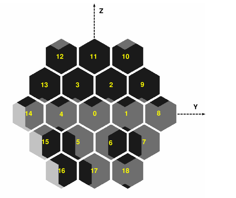
Figure 1: The shadowgram of the detectors plane of the SPI telescope in the simple case when only one source is located in the SPI FOV. The“black” colour corresponds to the area illuminated by the source ; “Dark grey” to the area shadowed by the mask; “Light grey – to the area closed for the source by the collimator.

2 Observations and data reduction

2.1 INTEGRAL

The International Gamma-Ray Astrophysics Laboratory (INTEGRAL; Winkler et al., 2003) was launched on Proton/Block-DM on October 17, 2002 into a geosynchronous highly eccentric orbit with high perigee (Eismont et al., 2003). The scientific payload of INTEGRAL includes four telescopes: the spectrometer SPI (Vedrenne et al., 2003), the imager IBIS (Ubertini et al., 2003), the X-ray monitor JEM-X (Lund et al., 2003) and the optical monitor OMC (Mas-Hesse et al., 2003).

2.1.1 The SPI telescope characteristics

In this paper, we focus on analysis of the SPI data. For detailed description of the instrument calibrations and performance, see Vedrenne et al. (2003), Atti$\acute{e}$ et al. (2003) and Roques et al. (2003). Below we give only a brief review of the key characteristics of the instrument and software relevant for this work.

SPI consists of 19 high purity germanium detectors (GeD) packed into a hexagonal array (see Figure 1). The combination of a good sensitivity to the continuum and line emission in the energy band $20-8000$ keV, provided by a large geometrical detector’s plane area ($\sim 500~{}cm^{2}$) and cryogenic system, and a good timing resolution ($102.4~{}\mu sec$) gives us an opportunity to study even very fast X/$\gamma$-rays pulsars.

There are two main types of SPI events: single events (registered by only one detector) and multiple events (scattered photon detected by two and more detectors). Though the pulsating signal is clearly detected in both types of events, we did not use the multiple events because of difficulties in the extraction of the spatial information, worse timing resolution and the lack of a tested energy response matrix. It should be noted that this kind of data was successfully used by Dean et al. (2008) for measuring Crab polarisation.

2.1.2 The SPI clock and time connection

SPI has its own internal clock, a 20MHz oscillator that generates time tag signal every 2048 periods, i.e. 102.4 $\mu s$ – the time resolution of the instrument. The SPI clock is synchronised with the on-board clock at every $125$ ms (the 8Hz on-board cycle, $OBT_{8Hz}$) by a reseting of the counter associated to the SPI oscillator. The SPI time tags are counted from the beginning of the 8Hz cycle and divide the $125$ ms interval into 1019 intervals of 102.4 micro seconds duration plus one interval with a duration of 70 micro seconds. In fact, the base frequencies of both on-board and SPI clocks are slightly varying with time (e.g. due to variation of the crystals temperature) that leads to variation in duration of SPI time tag intervals. We have estimated this effect to be very small ($<5~{}\mu s$ for any statistically significant analysis), neglected it and used the nominal values of the frequencies. The on-board time (OBT) of the current 8Hz cycle is the value of the datation of the beginning of the cycle (SPI User Manual - Issue 5.2 - SEP 2002). By convention, the On Board Time (OBT) of any event is the time of the leading edge of the interval where the event has been detected, that is :

$$OBT=OBT_{8Hz}+N_{tt}*D/2^{-20},$$ (1)

where $N_{tt}$ is the number of the SPI time tag interval ($0..1019$) and $D=102.4\times 10^{-6}s$ is the length of the interval. The divisor $2^{-20}$ is introduced to convert time expressed in seconds to on-board time units and reflects the conventional time resolution of the INTEGRAL clock (the real clock accuracy is $2^{-19}$ seconds). For the conversion of the On Board Time to Coordinated Universal Time (UTC) and for the barycentric correction we have used routines from the standard Off-line Science Analysis software package version 7.0 developed at INTEGRAL Science Data Centre (Courvoisier et al., 2003) and the time correlation files provided with the auxiliary data for the INTEGRAL data archive generation number 2. The equation (1) and the time transformation routines ensure accuracy of returning Universal Time of the order of $100~{}\mu s$. For precise timing analysis, a time correction must be added to OBT before any conversion:

$$\Delta T=\Delta T_{SPI}+\Delta T_{sat}+\Delta T_{rev2},$$ (2)

where $\Delta T_{SPI}=D/2=51.2~{}\mu s$ — the mean systematic shift due to the fact that the arrival time of events is defined as the time of the leading edge of the time tag interval, while the actual arrival times are normally distributed inside the time tag interval;
$\Delta T_{sat}=83~{}\mu s$ – the delay between the on-board time and SPI time (ground calibration, Alenia Spazio, 2002);
$\Delta T_{rev2}=-47~{}\mu s$ – this shift is common for all time correlation files from the archive generation 2 (will disappear in the new generation of archive).
Note, that the SPI instrumental delay given in the Table 4 of Walter et al. (2003) is the sum of the first two terms ($134~{}\mu s$) of the expression (2).

In our analysis, to avoid an additional discretization in time series we decided to define the time of any registered event not as the time of the leading edge of the appropriate time tag interval, but as a linearly randomised time inside this time tag interval, and the final expression for OBT is the following:

$$OBT=OBT_{8Hz}+\left((N_{tt}+rand[0,1])*D+\Delta T\right)/2^{-20},$$ (3)

in this case $\Delta T_{SPI}=0$ and therefore $\Delta T=+36\times 10^{-6}~{}s$.

Table 1: List of observations used in this analysis.

Rev.	Observing Period	Exp.a	Target b
No	UTC	ks
YEAR 2003
0043	$\bf 19.177-21.783$ Feb.	$\bf 164$	CRAB
0044	$\bf 22.163-24.772$ Feb.	$\bf 177$	CRAB
0045	$\bf 25.167-27.699$ Feb.	$\bf 162$	CRAB
0102	$\bf 14.623-17.218$ Aug.	$\bf 91$	CRAB
0103	$\bf 17.610-17.845$ Aug.	$\bf 22$	CRAB
0124	$\bf 19.430-22.031$ Oct.	$\bf 195$	IC443
0125	$\bf 22.422-25.023$ Oct.	$\bf 196$	IC443
0126	$\bf 25.414-28.015$ Oct.	$\bf 110$	IC443
YEAR 2004
0170	$\bf 5.122-7.302$ Mar.	$\bf 119$	CRAB
0182	$\bf 9.987-12.504$ Apr.	$\bf 197$	IC443
0184	$\bf 15.976-18.566$ Apr.	$\bf 222$	IC443
0239	$\bf 27.435-30.036$ Sep.	$\bf 187$	CRAB
0247	$\bf 21.363-23.964$ Oct.	$\bf 223$	IC433
YEAR 2005
0300	$\bf 28.910-31.504$ Mar.	$\bf 188$	CRAB
0352	$\bf 31.463-2.890$ Aug/Sep.	$\bf 200$	A0535
0365	$\bf 11.096-11.938$ Oct.	$\bf 59$	CRAB
YEAR 2006
0422	$\bf 28.729-31.198$ Mar.	$\bf 190$	CRAB
0464	$\bf 1.252-3.011$ Aug.	$\bf 60$	Taurus
0483	$\bf 28.711-29.627$ Sep.	$\bf 69$	CRAB
YEAR 2007
0541	$\bf 19.537-22.128$ Mar.	$\bf 213$	CRAB
0605	$\bf 27.016-28.927$ Sep.	$\bf 154$	CRAB
YEAR 2008
0665	$\bf 24.473-27.033$ Mar.	$\bf 194$	CRAB
0666	$\bf 27.463-30.022$ Mar.	$\bf 204$	CRAB
0727	$\bf 25.940-28.488$ Sep.	$\bf 197$	CRAB
0728	$\bf 28.932-1.499$ Sep./Oct.	$\bf 184$	CRAB
YEAR 2009
0774	$\bf 13.538--16.145$ Feb.	$\bf 196$	CRAB

^a – this value represents the total exposure of selected data
^b – for the complete description of the observations see the ISOC site http://www.sciops.esa.int

2.1.3 Data selection

In our analysis we have used publicly available data of all observations where the source was in the FOV of the SPI telescope. The exposure of selected data totals up approximately $4$ Ms.

SPI is a telescope with a coded mask aperture and most INTEGRAL observations are organised as a set of snapshots of the sky around a target (pointings or Science Windows – continuous observations pointed on a given direction in the sky). It means that the instrument effective area for the chosen target is changing from pointing to pointing. This effective area is mainly determined by geometrical area of the non-shadowed part of the detector plane (see Figure 1).

To extract the Crab pulsed signal we have used the epoch folding technique (Leahy et al., 1983). Any set of observations can be represented as a set of the whole detector plane count rates and in these terms, the total folded curve is the direct sum of the folded countrates of the individual pointings. To reach the best result we need to find an optimal series of the INTEGRAL pointings for which the signal to noise ratio will be the highest one. In this regard, several parameters characterise each pointing: the exposure of the pointing, $T_{i}$; the background conditions – the instrumental background countrate plus the sum of the countrates from other sources in the FOV, $C_{i}^{b}$; the illumination fraction of the detector plane, $\alpha_{i}$, corresponding to the source direction (could include not only geometrical factor, varies from 0 to $\sim 0.6$); and the mean countrate of the pulsating part of the source emission, $C_{i}^{p}$ (for completeness, below we are introducing also the term $C_{i}^{dc}$ - the mean unpulsating countrate of the pulsar, for the Crab pulsar $C_{i}^{dc}=0$). Using the terminology introduced above and assuming that all variances follow the Poisson statistic, the signal to noise ratio for the sequence of M pointings can be expressed as follows:

$$\left(\frac{S}{N}\right)_{M}=\frac{\sum\limits_{i=1}^{M}\alpha_{i}C_{i}^{p}T_{i}}{\sqrt{\sum\limits_{i=1}^{M}(C_{i}^{b}+\alpha_{i}(C_{i}^{p}+C_{i}^{dc}))T_{i}}}$$ (4)

The optimal set of K pointings chosen from the initial set of M pointings is that for which the value of $(S/N)_{K}$ calculated using the equation (4) reaches its maximum. In the case of a large number M the exhaustive search will take infinite time (even for $M=100$ the number of combinations exceeds $10^{30}$, in our case $M>1000$). Several simplifications have been investigated.

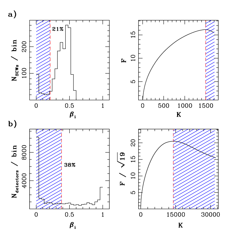
Figure 2: The left panels show the distribution of the number of SCWs (a) or the number of individual detectors (b) versus their illumination fraction for our data set. The function F(K) (see the equation (6)) is plotted on the rights panels for two cases: a) the whole detector plane; b) individual detectors. Shaded areas correspond to the data that should be excluded from the analysis. The function F in the case (b) is renormalised to be in the same units as in the case (a).

Considering that the INTEGRAL pointings (or Science Windows, SCWs) cover generally $\sim 2-5$ ks time intervals, we can treat the exposure $T_{i}$ of individual member of the data series as constant, i.e. $T_{i}\simeq const=T$, $i\in[1,M]$. Moreover, in the SPI telescope, the background dominates the useful signal, i.e. $(C_{i}^{p}+C_{i}^{dc})\ll C_{i}^{b}$ is true for any point source excluding the brightest events like Gamma-Ray Bursts or short intense bursts from Soft Gamma-Ray Repeaters and Anomalous X-ray Pulsars. Further, the amplitude of the variation of the SPI background does not exceed $\sim 50\%$ of its mean level (excluding periods of Solar flares). So, we can treat $C_{i}^{b}\simeq const=C_{b}$ for $i\in[1,M]$. We are assuming also that the mean value of the pulsar “Pulsed” component is constant in time $C_{i}^{p}\simeq const=C_{p}$. Now, taking into account assumptions listed above, we can modify the equation (4) as:

$$\left(\frac{S}{N}\right)_{M}\simeq\sqrt{\frac{TC^{2}_{p}}{C_{b}}}~{}\frac{\sum\limits_{i=1}^{M}\alpha_{i}}{\sqrt{M}}$$ (5)

In equation (5) we do not reduce the number of combinations in comparison with the equation (4) but now it is easy to see that the procedure of searching for the optimal set is equivalent to searching for the maximum value of the following discrete function:

$$F(K)=\frac{\sum\limits_{i=1}^{K}\beta_{i}}{\sqrt{K}},K\in[1,M]$$ (6)

where $B=[\beta_{i}]$ is the back ordered $A=[\alpha_{i}]$ set.

The speculations presented above could be easily extended to the case when we do not treat the whole detector plane (hereinafter referred to as the case I) but each detector separately (case II). In the latter case, $\alpha_{i}$ is the illumination fraction of an individual detector and varies in the range $0-1$, and M is the number of pointings times the number of the individual detectors (19 for SPI).

We have obtained the solution for our set of INTEGRAL observations for both cases as illustrated in Figure 2. To reach the maximum of the signal to noise ratio in case I, we should exclude from the analysis the pointings with an illumination fraction below $21\%$. In case II, we should use only those detectors that have an illumination fraction above $38\%$. Figure 2, shows that using individual detectors (case II) we obtain a $\simeq 30\%$ improvement of the signal detection significance. In this paper dedicated to the timing analysis, we have implemented case II.

2.2 Jodrell Bank Crab Pulsar Monthly Ephemeris

For the folding of the Crab pulsar lightcurves, we have used the time solution derived from Jodrell Bank Crab Pulsar Monthly Ephemeris (Lyne et al., 1993) and the corresponding Crab Pulsar coordinates. The database is available through the World Wide Web (http://www.jb.man.ac.uk/pulsar/crab.html) and contains the dispersion-corrected time of arrival of the centre of the main pulse (in TDB time system), the frequency and its first derivative and the range of validity. From this database we extracted the radio ephemerides covering the periods of the INTEGRAL observations. For each radio ephemeris record we took its two neighbours and calculated the second derivative of the frequencies so that the phases and frequencies given at the edge of the validity intervals and those deduced by extrapolation are consistent with each other better than $0.0001$ in phase and $10^{-7}$ in frequency. The resulting ephemerides for the INTEGRAL observing periods are given in Table 2.

The main pulse arrival time in the monthly ephemeris is determined with an error around $60~{}\mu s$, that includes the uncertainty in the delay due to interstellar scattering $\sim 20~{}\mu s$ (owing to the dispersion measure uncertainty $\Delta DM\sim 0.005~{}pc/cm^{3}$) as well as those arising from unknown instrumental effects $\sim 40~{}\mu s$ (see e.g. Rots et al. 2004 and references there). While the first part can be treated as a statistical error that follows the Poisson statistic and decreases with the number of independent measurements, the second part should be treated as a systematic error that is always present in the measured values.

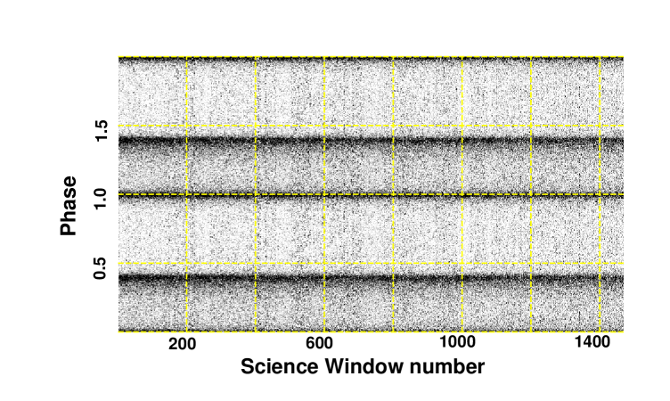
Figure 3: Science window by Science window folded curves in the 20-100 keV energy band. The folding procedure is based on ephemerides from the Table 2. No $\Delta\Psi$ correction is applied (see text).

2.3 RXTE

The PCA instrument onboard the RXTE (Rossi X-ray Timing Explorer) orbiting X-ray observatory consists of five identical proportional counters with a total area of 6500 cm², operating in the 2-60 keV energy range (Bradt et al., 1993). The accuracy of the RXTE clock in absolute time for our observing time interval (2003-2009 yy.) is better than $2~{}\mu s$ (see Rots et al. 2004 and references therein). Because of its large area and excellent time resolution and time accuracy, the instrument is sensitive enough to reconstruct a significant 400 bins phase curve of the Crab pulsar using an exposure of the order of 1 ks. We used Crab PCA observations that coincide in time (within two weeks) with any of our INTEGRAL observation and contain data in the Generic event mode format with time resolution better than $250~{}\mu s$. For the fine clock correction and barycenter correction we used faxbary script from the FTOOLS package that calls the axBary code (see e.g. the RXTE Guest Observer Facility). For the folding procedure we use the same routine and the same ephemerides as for SPI/INTEGRAL.

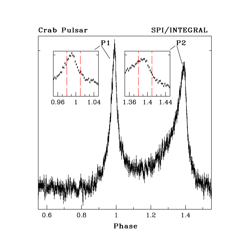
Figure 4: Crab phase histogram in the 20-100 keV energy band in absolute phase with the phase resolution of $0.0025$. “1” corresponds to the phase of the main radio pulse. Inner panels magnify the main pulse and the interpulse peaks. Dashed vertical lines bound the intervals used for the fit procedure. The exposure is of the order of 100 ks.

3 SPI/INTEGRAL analysis and results

To perform epoch folding analysis we ascribe to each detected photon the phase $\Psi_{t}$ using the appropriate ephemeris from the Table 2 and the following formula:

$$\Psi_{t}=\Psi_{0}+f(t-t_{0})+\frac{1}{2}(t-t_{0})^{2}\frac{df}{dt}+\frac{1}{6}(t-t_{0})^{3}\frac{d^{2}f}{dt^{2}}$$ (7)

where $t_{0}$, $f$, $\frac{df}{dt}$, $\frac{d^{2}f}{dt^{2}}$ is the radio ephemerides valid for the moment “t” and $\Psi_{0}\equiv 0$ (we want to work in absolute phase, i.e. the main radio pulse is at phase $0.0$). Then we can plot the phase values producing light curves with the requested resolution (here we use 400 bins per cycle). The middle of the zero bin is corresponding to the phase $0.0$.

As a first step, to check our SPI data set for the presence of unknown “glitches” from the Crab pulsar or some instrumental artifacts (e.g. inaccuracy in the on-board to Universal time conversion procedure) we folded separately each SCW lightcurve in the broad $20-100$ keV energy band. The result of the dynamical folding is presented on Figure 3, where we see that the shape of the Crab phase histograms and absolute phases are very stable (the two peaks of the pulse are good tracers).

In order to determine the phase of the hard X-ray main pulse and interpulse more precisely and to study possible variations of these values in time we summed up the SCW folded curves for each revolution. The SPI pulse profile for the Crab pulsar in the $20-100$ keV energy band for the exposure $\sim 100$ ks is presented on Figure 4. To define the phase of the pulses, we fitted the data for each revolution with a composite model: a Gaussian function plus a constant background, in the phase intervals $0.98-1.01$ and $1.38-1.41$ for the main pulse and interpulse, respectively, and adopted the fitted position of the Gaussian centroid as the appropriate phase of the corresponding pulse. To make sure that the fit results are model independent, we fitted the data for the main pulse with two other models: Lorentzian — used in Rots et al. (2004) (due to the lack of statistic for the one revolution timescale we could not apply the complete procedure of the peak-finding described in this paper) and Lorentzian plus constant — used in Kuiper et al. (2003). We found that all three models yield similar values, with dispersion not exceeding $0.0003$ period ($<10~{}\mu s$).

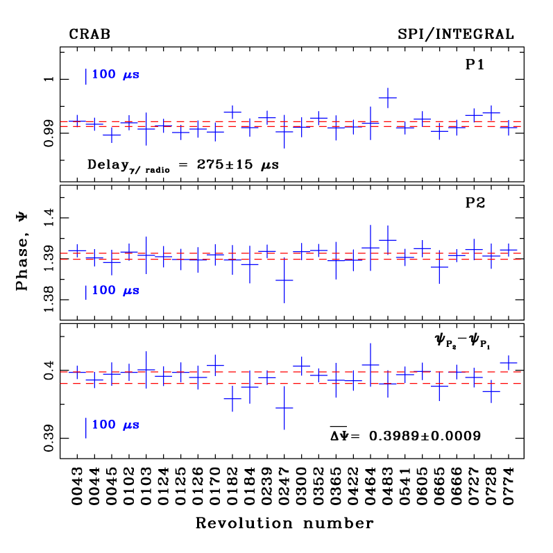
Figure 5: The best fit values of the main pulse (P1), interpulse (P2) positions and distance between them in the phase plane versus the revolution number, in the $20-100$ keV energy band. The horizontal dashed lines show the one sigma (statistical only) confidence intervals for the averaged values.

The absolute phases of the main pulse and interpulse (with respect to the radio main pulse) together with the phase difference between them, as a function of the observation number, are shown in Figure 5. The distributions of $\Psi_{P1}$ and $\Psi_{P2}$ values are well consistent with normal distributions ($\Psi_{P2}-\Psi_{P1}$ is not a measured value but a combination of two independent functions). The mean value of the hard X-ray main pulse phase is $0.99182\pm 0.00046$, thus, the pulse leads the radio main pulse by $8.18\pm 0.46$ milliperiods or $275\pm 15~{}\mu s$. Such quoted error does not include $40~{}\mu s$ coming from the uncertainty of the radio ephemeris. The average value of the two pulses separation is $0.3989\pm 0.0009$ parts of the cycle. Note, that this relative value is independent of any uncertainty in the radio timing ephemeris.

4 Comparison with PCA

For independent check of the hard X-ray results, we carried out the analogous analysis in the 2-20 keV energy band. We used the data of Crab observations with the PCA monitor quasisimultaneous with INTEGRAL. We used the same radio ephemeris and the same pulse definition procedure. The phase positions of the X-ray main pulse relative to the radio one for 79 PCA/RXTE observations are shown in the bottom panel of Figure 6, showing that also the main X-ray pulse leads the radio one. To determine the mean value of the time lag we approximated the PCA data with a constant and got $0.00933\pm 0.00016$ in phase units or $310\pm 6\mu s$ in time. Again we are quoting only statistical errors but we keep in mind the systematic $\sim 40\mu s$ error that comes from the radio ephemeris uncertainties. Based on two measured time lags “X-ray/radio” and “hard X-ray/radio” we can conclude that the main X-ray pulse is leading the hard X-ray main pulse by $35\pm 16\mu s$. This value differs only marginally from zero (we provided the one sigma error) even taking into account that in this case the radio error does not play a role since we used the same radio ephemerides for both measurements. Another quantity that is independent of any uncertainty in the radio timing ephemerides is the phase difference between the main pulse and interpulse. From our set of PCA/RXTE observations, we got a value of $0.40016\pm 0.00028$ that is in a good agreement with the result obtained in hard X-rays ($0.3989\pm 0.0009$, SPI/INTEGRAL).

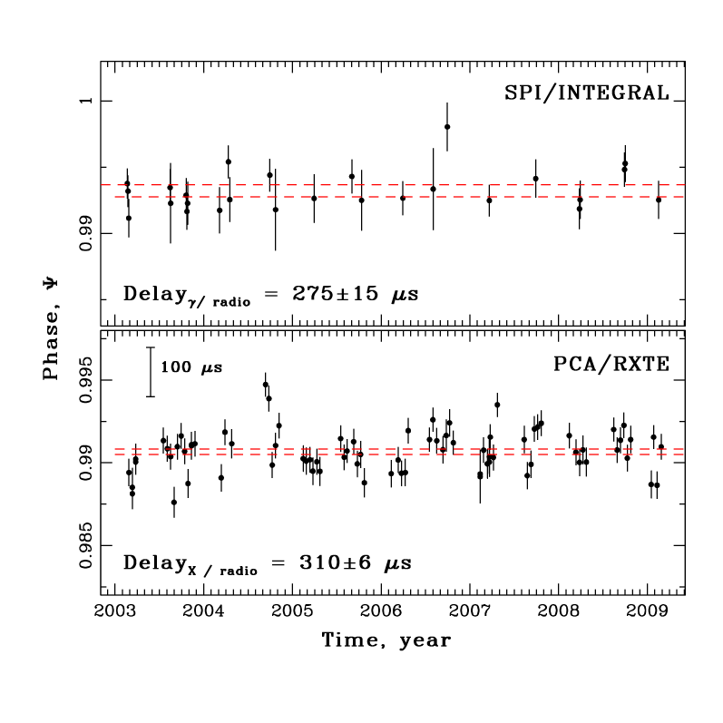
Figure 6: The main pulse maximum arrival phase in the $20-100$ keV energy band with SPI/INTEGRAL (1 point by time interval order of 100 ks), and in the $2-20$ keV energy band with PCA/RXTE (1 point — a few kiloseconds). The same radio ephemerides and fit procedure have been used. The horizontal dashed lines show the one sigma (statistical only) confidence intervals for the averaged values.

5 Radio delay evolution with energy

We have measured accurately the delays of the main pulse arrival time in wide $2-20$ keV (soft X-rays) and $20-100$ keV (hard X-rays) energy bands with respect to the radio main pulse arrival time. The $310\pm 6~{}\mu s$ soft X-ray/radio delay derived in this paper based on the PCA data (Rots et al. 2004 provides even higher value $344\pm 40~{}\mu s$) is marginally higher than the radio delay with respect to $275\pm 15~{}\mu s$ hard X-ray/radio delay measured with SPI. Both values are also slightly higher of the radio/optical delay of $255\pm 21~{}\mu s$ derived from S-Cam optical observations (Oosterbroek et al. 2008) and the $241\pm 29~{}\mu s$ radio/gamma one ($>30$ MeV, EGRET, Kuiper et al. 2003). To check whether this differences are real or not, we have made an additional analysis and investigated the behaviour of the radio delay with energy. The radio delay evolution with energy have been observed in optical wavelength (Oosterbroek et al. 2008), that gave us an extra motivation. We have built folded curves in narrower energy bands. We split the $2-20$ keV PCA energy band on three parts, while we used five energy channels to cover the 20-300 keV energy band for SPI data. We also added the High-Energy X-Ray Timing Experiment (HEXTE/RXTE) data in four energy bands covering the $20-250$ keV energy range, allowing a direct crosschecking with SPI results. The position of the main peak has been determined as previously, from a fit with a composite model: a Gaussian function plus a constant background, in the phase interval $0.98-1.01$. Figure 7 presents the evolution of the radio delay versus energy for the RXTE and SPI data, together with the optical and $\gamma-$rays points from Oosterbroek et al. (2008) and Kuiper et al. (2003). The decreasing trend of the radio delay with energy in the ($2-300$ keV) energy domain supports the reality of the delay measured between the soft X- and hard X-ray main peaks, even though the individual error bars are large. When modelling this decrease by a simple linear law (dashed line in Figure 7 ) we find that the radio delay decreases with a rate of $\sim 0.6\pm 0.2~{}\mu s/keV$. The obtained Chi2 of 7.1 for 10 dof compared to the value of 42.4 for 11 dof for a constant model corresponds to a probability of 3.5$\times 10^{-5}$ that its improvement is by chance.

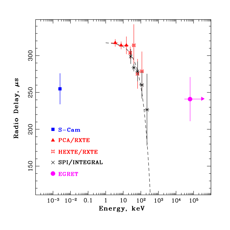
Figure 7: The radio delay in function of energy. The optical (S-Cam) and $\gamma-$ray (EGRET) points are from Oosterbroek et al. 2008 and Kuiper et al. 2003, respectively. The data of the RXTE instruments and SPI are from this work.

6 Discussion and conclusions

We have investigated the pulse profile of the Crab pulsar between 2 and 300 keV with PCA/RXTE instrument and SPI/INTEGRAL telescope. We found the strong indication that in this energy range the radio delay is significantly decreasing with energy. The simplest explanation of such a behaviour is that the $X-ray/\gamma_{soft}$-ray emission originates in a region extended along the open magnetic field lines, with softer photons originating at higher altitudes while the time offsets represent simply the path-length differences. In this case, the time delay determines the characteristic azimuthal size of the emitting area as $54\pm 18$ km.

It is clear that the radio delay can not decrease linearly through the full gamma rays range, since the EGRET point imposes a positive value. Moreover, contrary to we observe above 2 keV, the radio delay increases between optical and X-rays. It is interesting to note that the X-ray delay is consistent with the rate of $-5.9\pm 1.9~{}\mu s/1000~{}\AA$ derived from the $3920-8230~{}\AA$ optical waveband by Oosterbroek et al. (2008).

Even thought the dependence of the main pulse phase position on energy is complex, we can explain it with a rather simple scheme, where the pulsed emission consists of the superposition of two independent components having different phase distributions and energy spectra. Indeed, such an analytical model has been introduced by Massaro et al. (2000) to interprete the BeppoSAX data in the 0.1-300 keV energy band (see also improvements Massaro et al., 2006; Campana et al., 2009). In the optical up to $\gamma-$ray domain, this model includes: an “optical”, $C_{o}$ and an “X-ray”, $C_{x}$. The fractional part of the $C_{x}$ component increases in the main pulse with increasing energy from 1 keV up to a 1 MeV, then decreases up to $\sim 10$ MeV energy but is negligible below 1 keV and above 10 MeV. $C_{x}/C_{o}$ ratio behaviour following the same law as the Bridge/P1 ratio presented in Kuiper et al. (2001). Thereby, in the X-ray band, the $C_{x}$ component shifts the maximum of the pulse I $(C_{x}+C_{o})$ emission toward the radio maximum on the phase plane. It explains that the radio delay decreases with energy in X-rays while it keeps identical values in the optical and $\gamma-$ray wavebands where the $C_{x}$ component is negligible. Considering that the values of the radio delay are nearly the same in the optical wavelengths and $\gamma-$rays, where $C_{o}$ largely dominates over $C_{x}$, we can suggest that the $C_{o}$ component corresponds to a single emission mechanism and emission location from optical to $\gamma-$rays. In this case, the $\sim 250~{}\mu s$ radio delay indicates that the radio emission is produced in a region located closer from the Neutron Star by $\sim 75$ km than the $C_{o}$ production site. On the other hand, the $C_{x}$ component could be unrelated to the $C_{o}$ one, with a different origin and/or source location. In this case, the source behaviour in X-rays would result from a superposition of (at least) two independent components and the measured values of the radio delay in this energy band would not have any direct physical explanation.

Table 2: The Crab pulsar ephemerides for the INTEGRAL observations listed in Table 1. We used the Crab Pulsar position given in Jodrell Bank: $RA=83.633217^{\circ}$ and $DEC=22.014464^{\circ}$ in the J2000 epoch

Rev.	$T_{valid}$ (MJD),	$~{}f~{}~{}~{}~{}$,     Hz	$\Delta t_{0},\mu sec$	Rev.	$T_{valid}$ (MJD),	$~{}f~{}~{}~{}~{}$,     Hz	$\Delta t_{0},\mu sec$
No	$t^{Int}_{0}$ (MJD),	$~{}df/dt~{}~{}$, $10^{-10}$ sec-2	$\Delta\Psi$	No	$t^{Int}_{0}$ (MJD),	$~{}df/dt~{}~{}$, $10^{-10}$ sec-2	$\Delta\Psi$
	$t^{MP}_{0}$ (sec)	$d^{2}f/dt^{2}$, $10^{-21}$ sec-3			$t^{MP}_{0}$ (sec)	$d^{2}f/dt^{2}$, $10^{-21}$ sec-3
	$52671-52699$	$29.8092705147$	$18$		$53431-53461$	$29.7847841837$	$-19$
0043	$52685$	$-3.7366060$	$0.0005$	0300	$53444$	$-3.7315793$	$-0.0006$
	$0.076659$	$9.0$			$0.033023$	$6.0$
	$52671-52699$	$29.8092705147$	$-1$		$53584-53615$	$29.7798524524$	$36$
0044	$52685$	$-3.7366060$	$-0.0000$	0352	$53597$	$-3.7299236$	$0.0011$
	$0.076659$	$9.0$			$0.029626$	$9.0$
	$52671-52699$	$29.8092705147$	$-69$		$53644-53675$	$29.7778867428$	$-24$
0045	$52685$	$-3.7366060$	$-0.0021$	0365	$53658$	$-3.7294045$	$-0.0007$
	$0.076659$	$9.0$			$0.022656$	$4.0$
	$52852-52883$	$29.8034282349$	$8$		$53796-53826$	$29.7730221322$	$-19$
0102	$52866$	$-3.7350193$	$0.0002$	0422	$53809$	$-3.7278153$	$-0.0006$
	$0.018825$	$-1.0$			$0.005391$	$4.0$
	$52852-52883$	$29.8034282349$	$31.0$		$53917-53948$	$29.7690932051$	$4$
0103	$52866$	$-3.7350193$	$-0.0009$	0464	$53931$	$-3.7267461$	$0.0001$
	$0.018825$	$-1.0$			$0.020193$	$15.0$
	$52913-52944$	$29.8014598690$	$-11$		$53971-54009$	$29.7670971393$	$162$
0124	$52927$	$-3.7344076$	$-0.0003$	0483	$53993$	$-3.7264807$	$0.0048$
	$0.019997$	$3.0$			$0.011812$	$18.0$
	$52913-52944$	$29.8014598690$	$-52$		$54160-54191$	$29.7612711958$	$-25$
0125	$52927$	$-3.7344076$	$-0.0016$	0541	$54174$	$-3.7245631$	$-0.0007$
	$0.019997$	$3.0$			$0.020652$	$5.0$
	$52913-52944$	$29.8014598690$	$-31$		$54344-54374$	$29.7553516229$	$31$
0126	$52927$	$-3.7344076$	$-0.0009$	0605	$54358$	$-3.7225368$	$0.0009$
	$0.019997$	$3.0$			$0.010645$	$13.0$
	$53068-53074$	$29.7969173441$	$-50.0$		$54526-54557$	$29.7494993041$	$-46.0$
0170	$53071$	$-3.7535080$	$-0.0015$	0665	$54540$	$-3.7206976$	$-0.0014$
	$0.010486$	$350.0$			$0.008472$	$13.0$
	$53095-53105$	$29.7958809510$	$73$		$54526-54557$	$29.7494993041$	$-23$
0182	$53100$	$-3.7414057$	$0.0022$	0666	$54540$	$-3.7206976$	$-0.0007$
	$0.008622$	$200$			$0.008472$	$13.0$
	$53105-53115$	$29.7955577865$	$-22$		$54710-54741$	$29.7435856030$	$54$
0184	$53110$	$-3.7392771$	$-0.0007$	0727	$54724$	$-3.7189687$	$0.0016$
	$0.024904$	$-100$			$0.013181$	$17.0$
	$53255-53279$	$29.7906210263$	$40$		$54710-54741$	$29.7435856030$	$69$
0239	$53263$	$-3.7333983$	$0.0012$	0728	$54724$	$-3.7189687$	$0.0021$
	$0.021234$	$7.0$			$0.013181$	$17.0$
	$53279-53311$	$29.7896533932$	$-48.0$		$54863-54892$	$29.7386704404$	$-23$
0247	$53293$	$-3.7329692$	$-0.0014$	0774	$54877$	$-371735.72$	$-0.0007$
	$0.101225$	$9.9$			$0.000804$	$14.9$

References

- Alenia Spazio (2002) Alenia Spazio 2002, INTEGRAL End-to-End Timing Test Report, INT-RP-AI-0227, European Space Agency
- Atti et al. (2003) Atti, D., Gordier, B., Gros, M. et al. 2003, A&A, 411, L71
- Bradt et al. (1969) Bradt, H., Rappaport, S., Mayer, W., et al. 1969, Nature, 222, 728
- Bradt et al. (1993) Bradt, H.V., Rothschild, R. E., and Swank, J. H. 1993, A&AS, 97, 355
- Brandt et al. (2003) Brandt, S., Budtz-Jorgensen, C., Lund, N., et al. 2003, A&A, 411, L433
- Campana et al. (2009) Campana, R., Massaro, E., Mineo, T. and Cusumano, G. 2009, arXiv:0903.3655v1
- Courvoisier et al. (2003) Courvoisier, T.J.-L., Walter, R., Beckmann, V. et al. 2003, A&A, 411, L53
- Eismont et al. (2003) Eismont, N., Ditrikh, A., Janin, G. et al. 2003, A&A, 411, L37
- Fritz et al. (1969) Fritz, G., Henry, R.C., Meekins, J.F., et al. 1969, Science, 164, 709
- Kuiper et al. (2001) Kuiper, L., Hermsen, W., Gusumano, G. et al. 2001, A&A, 378, 918
- Kuiper et al. (2003) Kuiper, L., Hermsen, W., Walter, R. et al. 2003, A&A, 411, L31
- Kurfess (1971) Kurfess, J.D., 1971, ApJ, 168, L39
- Leahy et al. (1983) Leahy, D. A., Darbro, W., Elsner, R. F., et al. 1983, ApJ, 266, 160
- Lund et al. (2003) Lund, N., Brandt, S., Budtz-Jorgensen, C., et al. 2003, A&A, 411, L231
- Lyne et al. (1993) Lyne, A. G., Pritchard, R. S. and Graham-Smith, F. 1993, MNRAS, 265, 1003
- the MAGIC collaboration (2008) The MAGIC collaboration 2008, Science, 322, 1221
- Mas-Hesse et al. (2003) Mas-Hesse, M., Gimenez, A., Culhane, L., et al. 2003, A&A, 411, L261
- Masnou et al. (1994) Masnou, J. L., Agrinier, B., Barouch, E., et al. 1994, A&A, 290, 503
- Massaro et al. (2000) Massaro, E., Cusumano, G., Litterio, M and Mineo, T. 2000, A&A, 361, 695
- Massaro et al. (2006) Massaro, E., Campana, R., Cusumano, G., and Mineo, T. 2006, A&A, 459, 859
- Moffett and Hankins (1996) Moffett, D. A., and Hankins, T. H. 1996, ApJ, 468, 779
- Nolan et al. (1993) Nolan, P. L., Arzoumanian, Z., Bertsch, D. L., et al. 1993, ApJ, 409, 697
- Oosterbroek et al. (2008) Oosterbroek, T., Cognard, I., Golden A. et al. 2008, A&A, 488, 271
- Pravdo et al. (1997) Pravdo, S. H., Angelini, L., and Harding, A. K. 1997, ApJ, 491, 808
- Roques et al. (2003) Roques, J. P., Schanne, S., von Kienlin, A., et al. 2003, A&A, 411, L91
- Rots et al. (2004) Rots, A. H., Jahoda, K., and Lyne A. G. 2004, ApJ, 605, L129
- Thompson et al. (1977) Thompson, D. J., Fichtel, C. E., Hartman, D.,A., et al. 1977, ApJ, 213, 252
- Ubertini et al. (2003) Ubertini, P., Lebrun, F., Di Cocco, G., et al. 2003, A&A, 411, L131
- Vedrenne et al. (2003) Vedrenne, G., Roques, J. P., Sch nfelder, V., et al. 2003, A&A, 411, L63
- Walter et al. (2003) Walter, R., Favre, P., Dubath, P., et al. 2003, A&A, 411, L25
- White et al. (1985) White, R. S., Sweeney, W., Tumer, T. and Zych, A. 1985, A&A, 299, L23
- Wills et al. (1982) Wills, R. D., Bennett, K., Bignami, G. F., et al. 1982, Nature, 296, 723
- Winkler et al. (2003) Winkler, C., Courvoisier,T.J.-L., Di Cocco, G., et al. 2003, A&A, 411, L1