Abstract

I tackle the problem of partitioning a sequence into homogeneous segments, where homogeneity is defined by a set of Markov models. The problem is to study the likelihood that a sequence is divided into a given number of segments. Here, the moments of this likelihood are computed through an efficient algorithm. Unlike methods involving Hidden Markov Models, this algorithm does not require probability transitions between the models. Among many possible usages of the likelihood, I present a maximum a posteriori probability criterion to predict the number of homogeneous segments into which a sequence can be divided, and an application of this method to find CpG islands.

1 Introduction

An important element in analysing a sequence of letters is to find out whether the sequence has a structure, and if so, how it is structured. Usually, looking for structure in a sequence implies a partition – or segmentation – in which each segment can be considered “homogeneous”, on the basis of a specific criterion. There are two main approaches to tackle this problem (Braun and Müller,, 1998).

A commonly used methodology is to model the sequence with Markov models. A Markov model gives, for each word of a given length, the probabilities of letters conditionally following this word – called emission probabilities. The likelihood of a segment of letters is the product of these probabilities at all the positions of the segment. Various models give different likelihoods for a given segment, some of them greater than others. Looking for a segmentation of a sequence means dividing it into segments, so that a model chosen as the best from amongst a set of models is attributed to each segment. One way to study the structure of a sequence is to analyse the set of its segmentations.

To make this task possible, the set of models is usually organized to form a Markov meta-model in which there are transition probabilities between the models. This is known as a Hidden Markov Model (HMM). In this context, the models are usually called states, but for the sake of consistency I keep the same vocabulary as before. In an HMM, a run of models is a Markov process with a probability, and, given a run of models, the sequence has a likelihood. If a segment is defined as a range of positions modelled by a unique model, it is possible to compute the probability of a segmentation given the sequence and the HMM. As this method permits efficient (i.e. with linear complexity) algorithms for sequence analysis and partitioning (Rabiner,, 1989), it is used in numerous applications, for example in bioinformatics (Churchill,, 1989; Baldi et al.,, 1994; Lukashin and Borodovsky,, 1998; Peshkin and Gelfand,, 1999; Nicolas et al.,, 2002; Boys and Henderson,, 2004) and in speech recognition (Ostendorf et al.,, 1996).

However, since in an HMM the chain of the models is markovian, the lengths of the segments defined by the models are expected to follow geometric laws, which may be a false hypothesis for real data segments. Various solutions have been proposed to overcome this problem, such as using semi-Markov chains (Guédon,, 2005) or macro-states (Ephraim and Merhav,, 2002), but in fact they make the modelling task more complex, since more parameters are used to obtain a better modelling of the lengths of the segments. Moreover, in the problem of sequence segmentation using a set of models, the inter-model transition probabilities used in an HMM correspond to an a priori on the distributions of the segments, and are superfluous parameters if we consider that the models themselves should be sufficient to segment the sequence, as in the approach described below. Finally, in an HMM, the models modelling and the length modelling can be seen as two competing modellings, because in the parts of the sequence where the models do not discriminate clearly, the length parameters will have a predominant influence. This is even more problematic when the lengths of the real segments are very different along the sequence.

A way to avoid these “extra” parameters is to establish a homogeneity criterion for a segment (such as the variance of its composition, or its maximum likelihood given specific models), and to determine a set of segments that divide the sequence and minimize – or maximize – this criterion. This problem – also known as the changepoint problem – can be solved by an optimal algorithm (Bellman,, 1961), but its time-complexity is quadratic with the length of the sequence, which prohibits the analysis of very long sequences. Alternatively, this problem can be tackled linearly using hierarchical segmentation (Li et al.,, 2002; Li,, 2001), or with approximations about the limits of the segments (Barry and Hartigan,, 1993; Braun et al.,, 2000), but these approaches do not ensure that the best partition is found. Moreover, when the homogeneity criterion is monotonous with the number of segments (such as the maximum likelihood of markovian processes), these methods need an additional criterion to stop the segmentation process. For each number of segments, the calculation of the criterion is based on the built partition and is very dependent on the choice of this partition. Without a stopping criterion, these methods produce multi-level descriptions of the structure of the sequences that may be quite interesting, but I am not aware of any practical usage of such sets of segmentations.

Between those two approaches, I described in  (Guéguen,, 2001) an algorithm – known as MPP, or Maximal Predictive Partitioning – that computes the most likely segmentation of a sequence in $k$ segments given a set of Markov models. This algorithm is optimal and has a time-complexity linear with the length of the sequence. As with the previous segmentation methods, it provides a multi-level description of the structure of a sequence, and it needs an additional criterion to select the “best” partition, such as the number of segments.

Bayesian methods are a different approach to work on sequence segmentation, since they propose to simulate the a posteriori distribution of the segmentations of a sequence, given a criterion (Liu and Lawrence,, 1999; Salmenkivi et al.,, 2002; Makeev et al.,, 2001; Keith,, 2006). Even though they do not construct the best segmentation, they indicate the relative significance of the segmentations, and the structuring of the sequence. Nonetheless, as the set of segmentations is very large, the convergence of the simulated distribution towards the right one can be extremely slow.

I would now like to look at the problem of estimating the structuring of a sequence given a set of Markov models. In contrast to the situation for an HMM, I do not want to put any constraint on the transitions between the models. This article presents an algorithm that computes the moments of the likelihood of a sequence under the set of all partitions with a given number of segments. The maximum of this likelihood was already computable with the MPP algorithm (Guéguen,, 2001). Since the time-complexity of this new algorithm is linear with the length of the sequence, it can also be applied to very long sequences.

The distribution of this likelihood may be useful for many statistical analyses of sequences, for example in an HMM modelling to test for the relevance of inter-model transition probabilities, or in a change point problem to test the significance of partitions and stop the partitioning, or in a bayesian approach to perform more efficient simulations of the a posteriori distribution of the segmentations of a sequence. As an example, I propose a maximum a posteriori estimator of the numbers of segments in a sequence.

2 Method

2.1 Computing the likelihood of the sequence

The method computes the moments of the likelihood that a sequence is partitionned in exactly $k$ segments given a set of Markov models. The algorithm that is presented permits the computation of the mean of this distribution. Generalizing this to the computation of all moments is straightforward.

First, we introduce some notations and concepts.

The studied sequence, ${\cal S}$, consists of letters, and has a length $l$. For all $i\in[0,l-1]$, we denote by ${s}_{i}$ the $i$-th letter of ${\cal S}$, and ${\cal S}_{i}$ the segment of ${\cal S}$ from position $0$ to position $i$, inclusive. ${\cal S}={\cal S}_{l-1}$.

A $k$-partition is a partition in $k$ segments. A predictive $k$-partition is a $k$-partition in which a model is associated with each segment, and neighbouring segments have different models. The set of the predictive $k$-partitions of ${\cal S}$ is denoted $\mathbb{P}_{k}$. From here on, all partitions will be predictive partitions.

Let us call the set of models $D$; for all $d\in D$ we denote by $\pi_{d}(i)=\text{pr}({s}_{i}|{\cal S}_{i-1},d)$ the probability of the $i$-th letter given the model $d$ and the previous $i-1$ letters of the sequence. The likelihood of a segment $\sigma\subset{\cal S}$ given a model $d\in D$ is the product of the likelihoods of its letters $\text{pr}(\sigma|d)=\prod_{{s}_{i}\in\sigma}\pi_{d}(i)$. For $p$ in $\mathbb{P}_{k}$, the likelihood of ${\cal S}$ given $p$, $\text{pr}({\cal S}|p,D)$, is the product of the likelihoods of the predictive segments of ${\cal S}$ defined by the partition. We have defined a distribution of the likelihoods over $\mathbb{P}_{k}$, $(\text{pr}({\cal S}|p,D))_{p\in\mathbb{P}_{k}}$, and we are looking for the expectation of this distribution $\text{pr}({\cal S}|\mathbb{P}_{k},D)=\sum_{p\in\mathbb{P}_{k}}\text{pr}({\cal S}|\mathbb{P}_{k},D).\text{pr}(p|\mathbb{P}_{k})$.

We denote $m_{k}(i)$ the expectation of the likelihoods of ${\cal S}_{i}$ under the set of the $k$-partitions of ${\cal S}_{i}$, and $m_{k}^{d}(i)$ is the expectation of the likelihoods of ${\cal S}_{i}$ under the set of the $k$-partitions of ${\cal S}_{i}$ whose model of the last segment is $d$. These values can be computed with a dynamic programming algorithm (the demonstration of which is appended):

$\displaystyle\forall i\geqslant 0,m_{1}^{d}(i)$ $\displaystyle=$ $\displaystyle\text{pr}({\cal S}_{i}|d)$ $\displaystyle\forall k\geqslant 1,\forall i<k-1,m_{k}(i)$ $\displaystyle=$ $\displaystyle 0$ $\displaystyle\forall k\geqslant 1,\forall i\geqslant k-1,m_{k}(i)$ $\displaystyle=$ $\displaystyle\frac{1}{\#D}\sum_{d\in D}m_{k}^{d}(i)$ $\displaystyle\forall k\geqslant 2,\forall i\geqslant k-1,m_{k}^{d}(i)$ $\displaystyle=$ $\displaystyle\pi_{d}(i).\bigg{(}\frac{i-k+1}{i}.m_{k}^{d}(i-1)$ $\displaystyle+\frac{k-1}{i.(\#D-1)}\left(\#D.m_{k-1}(i-1)-m_{k-1}^{d}(i-1)\right)\bigg{)}$

As $\text{pr}({\cal S}_{i}|d)$ is the likelihood of a segment given a specific model, it is computable. We can see that when $i=k-1$, the first term inside the brackets equals 0, which means that $m_{k}^{d}(i)$ can be recursively computed.

For each $k$, $\text{pr}({\cal S}|\mathbb{P}_{k},D)=m_{k}(l-1)$ is the mean likelihood of ${\cal S}$ under the set of the $k$-predictive partitions.

When, in the previous formula, we change $\pi_{d}(i)$ by $\pi^{\alpha}_{d}(i)$, the expectation of the $\alpha$th power of the likelihood of ${\cal S}$, $E_{p\in\mathbb{P}_{k}}(\text{pr}({\cal S}|p,D)^{\alpha})$, is computed, which is the $\alpha$-th moment around $0$ of this distribution. When $\alpha$ is a natural, it is then easy to compute the $\alpha$-th moment around the mean, such as the variance.

This algorithm has a linear time-complexity with the product of the number of models and the length of the sequence. Hence these likelihoods are quite computable, even for very long sequences.

2.2 Estimating the a posteriori probabilities

Considering the segmentation problem, we are actually interested in the a posteriori probability of the number of segments given the sequence, say $N$. We hypothesize hereafter that the probability of this number is equal to $\text{pr}(\mathbb{P}_{N}|{\cal S},D)$, even though this hypothesis deserves a closer examination. However, it is reasonable to assume that $\text{pr}(N|{\cal S},D)$ and $\text{pr}(\mathbb{P}_{N}|{\cal S},D)$ have the same modes, and that a maximal a posteriori estimator of $\text{pr}(\mathbb{P}_{N}|{\cal S},D)$ will be a maximal a posteriori estimator of $\text{pr}(N|{\cal S},D)$.

Owing to the bayesian formula $\text{pr}(\mathbb{P}_{N}|{\cal S},D)\propto\text{pr}({\cal S}|\mathbb{P}_{N},D)\text{pr}(\mathbb{P}_{N}|D)$, an a priori on the distribution of $\text{pr}(\mathbb{P}_{N}|D)$ has to be set. If this a priori is uniform with $k$, the a posteriori probability is directly proportional to the likelihood computed in the previous section: $\text{pr}(\mathbb{P}_{N=k}|{\cal S},D)\propto\text{pr}({\cal S}|\mathbb{P}_{k},D)$.

Another a priori is analogous to the HMM modelling: we consider that the segment length follows a geometrical distribution with a given mean, say $\lambda$. Then a priori $N-1$ follows a binomial distribution of parameter $\frac{\lambda}{l}$, and if we define a random variable $X\leadsto\text{Bin}(l,\frac{\lambda}{l})$, $\text{pr}(\mathbb{P}_{N=k}|{\cal S},D)\propto\text{pr}({\cal S}|\mathbb{P}_{k},D).\text{pr}(X=k-1)$.

A more experimental approach is to consider that $\text{pr}(\mathbb{P}_{N}|{\cal S},D)$ follows a given law with some parameters, and to simulate sequences generated by $k$-partitions to fit at best these parameters, considering an optimization criterion. An obvious criterion is to minimize the mean square error of the maximum a posteriori estimation of the numbers of segments.

2.3 Implementation

This algorithm has been implemented in C++, and is freely available via python modules in Sarment (Guéguen,, 2005) at the URL:
http://pbil.univ-lyon1.fr/software/sarment/

The examples of the next section are described in the tutorial at the same location.

3 Maximum a posteriori estimation

3.1 The a priori distribution

To build a good a posteriori estimator, we still need to look for a relevant a priori probability on the $\mathbb{P}_{k}$. To test this, I have generated random sequences made up of an alphabet of two letters (A and B), from several Markov models and random $k$-partitions, for several values of $k$. We denote $\text{Bern}(\alpha)$ the model where the emission probability of an A is $\alpha$ (and that of a B is $1-\alpha$). The positions of the limits of the segments were uniformly generated, so that each segment was at least 50 positions long, and the models were uniformly assigned to each segment so that no two neighbouring segments shared the same model. For each $k$, 100 random $k$-partitions and sequences 10,000 letters in length have thus been generated. To understand how the algorithm performs on more or less strongly segmented sequences, the next examples present sequences generated from models $\text{Bern}(0.3)$ and $\text{Bern}(0.7)$, and sequences generated from more similar models $\text{Bern}(0.4)$ and $\text{Bern}(0.6)$. The same models have been used to compute the likelihoods.

First, I searched for the number of segments $N$ for which the sequence has the highest likelihood. It is equivalent to the uniform a priori distribution.

The examples of log-likelihoods in Fig. 1 show a typical behaviour: the neighbourhood of the maximum likelihood can be reached very quickly, and there are several numbers of segments with a likelihood “near” this maximum. If in the left example, the maximum is reached on the exact number of segments, this maximum is reached for a higher number in the right example.

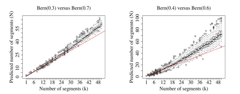
Figure 2: Boxplots of the numbers of segments $N$ reaching the maximum likelihood of the sequence, for a simulated number of segments $k$ between 1 and 50. The oblique line represents the right number of segments ($N=k$).

Actually, overall, the predicted numbers of segments are in accordance with the simulated numbers (Fig. 2). However, as the segments become more difficult to discriminate (when the average size of the simulated segments decreases or when the models generating the segments are more similar), the predicted number tends to over-estimate. This means that the number of segments with the highest likelihood is not in fact the one most relevant for this prediction, and another a priori than the uniform distribution should be chosen.

The a priori can be based on the length of the segments, as it is done in HMM modelling. Since in the simulations the inter-segments positions of the random partitions were uniformly taken along the sequence, the lengths of the simulated segments followed a geometric distribution, which should favour the analysis through HMM.

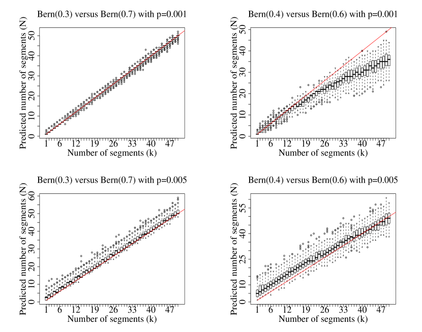
Figure 3: Boxplots of the numbers of segments $N$ predicted by the forward-backward algorithm, for a simulated number of segments $k$ between 1 and 50. The oblique line represents the right number of segments ($N=k$).

I have studied these sequences with the likelihood algorithm and with an HMM. The HMM used had the exact Markov models and an additional parameter $p$ on the probability transitions between the states, so that the average length of the segments is $1/p$. To get the resulting partition, I have applied the forward-backward algorithm on the sequences and successive positions were clustered in a segment when their most likely state was identical. Since the sequences were 10,000 letters long, the number of predicted segments minus one follows the binomial law $\text{Bin}(9999,p)$. I used $p=0.001$ (10 segments) and $p=0.005$ (50 segments), and again models $\text{Bern}(0.3)$ versus $\text{Bern}(0.7)$ and $\text{Bern}(0.4)$ versus $\text{Bern}(0.6)$ (Fig. 3).

Figure 3 shows that when the models are distant ($\text{Bern}(0.3)$ versus $\text{Bern}(0.7)$), the forward-backward algorithm performs rather well. However, with $p=0.005$ the number of segments is more over-estimated than with $p=0.001$, since it tends to increase the number of segments. When the models are less different, as with $\text{Bern}(0.4)$ versus $\text{Bern}(0.6)$, the influence of $p$ becomes critical. In this example, $p=0.001$ under-estimates the number of segments when the real number is over $10$, since this parameter means that a priori on average the sequence has $10$ segments. With $p=0.005$ the predictions over-estimate slightly for small numbers of segments, and they tend to under-estimate as the real number increases.

We can see that when this estimator is biased, the bias depends on the value of the inter-state probability and on the real number of segments in the sequence, which is not known beforehand.

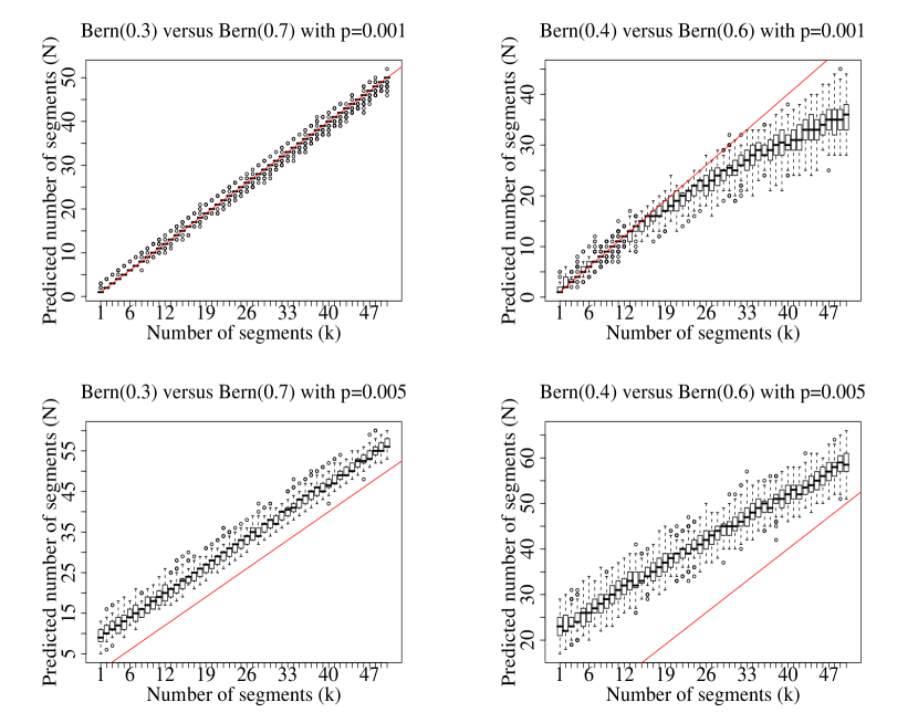
Figure 4: Boxplots of the numbers of segments $N$ with the maximum a posteriori probability, with a binomial a priori distribution on $\text{pr}(\mathbb{P}_{N}|D)$, for a simulated number of segments $k$ between 1 and 50. The oblique line represents the right number of segments ($N=k$).

Nonetheless, to study the effect of this a priori on the maximum a posteriori estimator, I have set the same binomial a priori distribution on $\text{pr}(\mathbb{P}_{N}|D)$, with $p=0.001$ and $p=0.005$. We can see in Fig. 4 the same behaviour as with the HMM modelling, but with a much more important over-estimation of the number of segments when $p=0.005$. It means that the tendency of this a priori to “drag” the maximum a posteriori towards 50 segments is here more influential. When the real number of segments is near 50, the over-estimation is lower than in Fig. 2, for the same reason. Then, even though it corresponds to the modelling of HMM, a binomial a priori is not relevant for maximum a posteriori estimation of the number of segments.

An experimental way to set up an a priori distribution is to define it through a set of parameters, that will be optimized by simulations. The optimization function is the minimization of the mean square error between the maximum a posteriori estimation and the real numbers $k$ of segments, summed for all $k$ from 1 to 50.

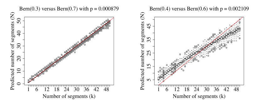
Figure 5: Boxplots of the numbers of segments $N$ with the maximum a posteriori probability, with a binomial a priori distribution on $\text{pr}(\mathbb{P}_{N}|D)$ and an optimized parameter $p$, for a simulated number of segments $k$ between 1 and 50. The oblique line represents the right number of segments ($N=k$).

A first way would be to optimize the parameter of the binomial a priori distribution. Indeed, the poor efficiency of these examples could be due to a bad parameter value. In these simulations, the optimal value $p$ is $0.00098$ (resp. $0.0021$) for the models $\text{Bern}(0.3)$ versus $\text{Bern}(0.7)$ (resp. $\text{Bern}(0.4)$ versus $\text{Bern}(0.6)$). The first optimization is quite efficient (Fig. 5) but when the segments are less different there is an over-estimation of the number of segments for small $k$, and an under-estimation for large $k$, as in the previous section. The correct estimations are around 25 segments, a balance between over-estimating and under-estimating all the $k$ between 1 and 50. Then even with an optimization process, a binomial a priori does not give an efficient a posteriori estimator.

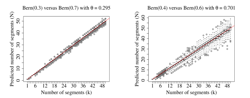
Figure 6: Boxplots of the numbers of segments $N$ with the maximum a posteriori probability, using an a priori distribution ${\cal G}(\theta)$ with an optimized $\theta$, for a simulated number of segments $k$ between 1 and 50. The oblique line represents the right number of segments ($N=k$).

I tried the same kind of optimization with a geometric a priori distribution ${\cal G}(\theta)$: $\text{pr}(\mathbb{P}_{N=k}|D,{\cal S})\propto\text{pr}({\cal S}|\mathbb{P}_{k},D).\theta^{k}$. I have performed twice the same round of sequence simulations as before, one set for the optimization of the parameter, and one set to test it on the obtained estimator. On these examples, when the models are distant enough, as in $\text{Bern}(0.3)$ versus $\text{Bern}(0.7)$, the estimator is quite accurate, and it is unbiaised, even with $\text{Bern}(0.4)$ versus $\text{Bern}(0.6)$ models (Fig. 6).

This example shows that this approach can give good results, even though it is up to now only experimental. A theoretical study may be useful to set up an even more efficient a priori, and to prevent the cost of simulations as well as the numerical optimization process. We can expect this distribution to depend on the set of models and on the length of the sequence, and it would be quite interesting to study it thoroughly.

3.2 CpG islands

In vertebrate genomes, CpG dinucleotides are mostly methylated and this methylation entails an hypermutability of these nucleotides, from CpG to TpG or CpA. A usual measure of this feature is to compute the ratio of the observed CpG dinucleotides over the expected number when the nucleotides are independent:

$$\textrm{CpGo/e}=\frac{\textrm{frequency of CpG }}{\textrm{frequency of C }\times\textrm{frequency of G}}$$

In some stretches of DNA, known as CpG islands, the CpG dinucleotides are hypomethylated. These islands are often associated with promoter regions (Ponger et al.,, 2001). They show a higher CpGo/e than surrounding sequences, at least $0.6$. Moreover, a CpG island is expected to be at least 300 bases long. I wanted to segment a sequence of the mouse genome to reveal the occurences of CpG islands. The CpGo/e ratio on this sequence is shown in 1,000 bases sliding windows (Fig. 7 middle).

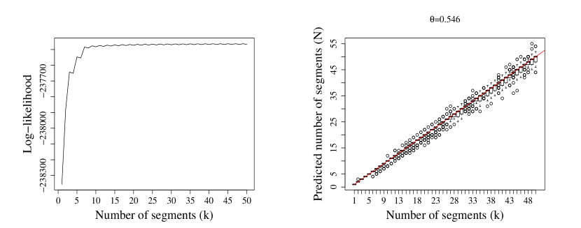
Figure 8: Study of a mouse sequence under the set of the $k$-partitions, given the CpG island vs non-Cpg island models. Left: Log-likelihood of the sequence, for $k$ numbers of segments, with $k$ between 1 and 50. Right: Boxplots of the numbers of segments $N$ with the maximum a posteriori probability, with a geometric a priori distribution ${\cal G}(0.546)$, for a simulated number of segments $k$ between 1 and 50. The simulated sequences were the same length than the studied one (176973), and the segments were at least 300 long. The oblique line represents the right number of segments ($N=k$).

As described by Durbin et al., (1998), I defined two first-order Markov models, built by maximum likelihood on known data: the first is trained on CpG islands, and the other on segments that are between the CpG islands. I used those models to compute the segmentation likelihood on a sequence of the mouse genome (Fig. 8), for up to 50 segments.

I looked for the maximum a posteriori estimator of the number of segments, with a geometric a priori distribution, and I simulated random sequences through the same process as described in section 2.3. The optimization of the maximum a posteriori estimator gives $\theta=0.546$, and the result of this optimization is shown in Fig. 8. We can see that this estimator is still unbiased until 50 segments, and quite precise.

With this a priori, the maximum a posteriori estimator on the mouse sequence gives 17 segments, and CpG-islands predicted in the most likely $17$-partition are shown in Fig. 7 bottom.

4 Discussion

In this article, I propose an algorithm to compute the moments of the likelihood of segmentation of a sequence in a number of segments, given a set of Markov models. This algorithm has a time-complexity linear with the length of the sequence and the number of models, and it can be used on very long sequences.

From this likelihood, it should be possible to compare the numbers of segments to partition a sequence, either through statistical tests or through a bayesian approach. In a bayesian approach, the a priori distribution of the numbers of classes must be defined, and I give some examples where a geometric a priori distribution gives a quite precise maximum a posteriori estimator. This has been only validated with simulations, and a full theorerical study is yet to be undertaken on the a priori distribution. Moreover, it would be quite interesting to define some statistical tests to assess the relative significance – confidence intervals and p-values – of the numbers of segments, given the models and the sequence. The fact that the moments of the distribution of the likelihood can be computed could be useful for this, as well as for an improvement of the previous estimator.

This algorithm does not put any constraint on the succession of models, but works as if the transition graph between the models were a clique. It is easy to see from the Appendix that it can be adapted to any kind of transition graph, which means that it may be useful in the context of HMM analysis, for example to check – or determine – the inter-model probabilities of the models, given a sequence. In this context, it could also be interesting to use the likelihood to enhance the efficiency of methods related to HMM modelling, for example for post-analysis of forward-backward algorithm. As in HMM modelling, one aim would be to compute the probability that a position is predicted by a model, given a set of models, and possibly given a number of segments. If the MPP algorithm is equivalent to the Viterbi algorithm for HMM, computing this probability would be the equivalent of the forward-backward algorithm in this context.

Even if model inference is out of the topic of this article, it is a very important feature in sequence analysis, and it will be interesting to use the likelihood for this. In Polansky, (2007), there is an example of inference of Markov models from a sequence, out of the context of HMM, but it is practically limited with the numbers of segments in the sequence and, since it uses the maximum likelihood, an additional penalization criterion (AIC or BIC) is necessary to handle this number. It should be possible to use the calculation of the average likelihood to get rid of these problems. Another inference process is the maximization, among a set of models, of the average likelihood. Moreover, it would be relevant to use the bayesian approach to estimate and simulate a posteriori probabilities for the parameters of the models, given the sequence.

Finally, as I said in the introduction, to my knowledge multi-level segmentations of sequences are not used for sequence analysis, although its relevance. An important barrier to this is the lack of evaluation criteria for these levels. Computing the likelihood for the successive numbers of segments may then be a quite useful tool to develop this kind of methodology. It would bring out a much richer modelling of the sequence.

Disclosure Statement

No competing financial interests exist.

Appendix

Here is a demonstration of the formula described in section 2, keeping the same notations:

We define

• $\mathbb{P}_{k}(i)$ the set of the $k$-partitions of ${\cal S}_{i}$

• $\mathbb{P}_{k}^{d}(i)$ the set of the $k$-partitions of ${\cal S}_{i}$ whose model of the last segment is $d$.

$m_{k}(i)$ is the likelihood of ${\cal S}_{i}$ under $\mathbb{P}_{k}(i)$, $\forall k\geqslant 0,\forall i\geqslant k-1,m_{k}(i)=\text{pr}({\cal S}_{i}|\mathbb{P}_{k}(i))$, and $m^{d}_{k}(i)$ is the likelihood of ${\cal S}(i)$ under $\mathbb{P}_{k}^{d}(i)$, $\forall k\geqslant 0,\forall i\geqslant k-1,m^{d}_{k}(i)=\text{pr}({\cal S}_{i}|\mathbb{P}^{d}_{k}(i))$

If the a priori on the last model $d$ is uniform:

$$m_{k}(i) = \text{pr}({\cal S}_{i}|\mathbb{P}_{k}(i))=\sum_{d\in D}m_{k}^{d}(i).\text{pr}(\mathbb{P}_{k}^{d}(i)|\mathbb{P}_{k}(i))$$ (1)

$$= \frac{1}{\#D}\sum_{d\in D}m_{k}^{d}(i)$$

We follow a bayesian approach, in which, for each $k$, all the $k$-partitions are equiprobable in $\mathbb{P}_{k}$.

If we note $d_{p}(i)$ the model used in partition $p$ at position $i$, we have for all $k\geqslant 2$ and $i\geqslant k-1,$

$$m_{k}^{d}(i) = \text{pr}({\cal S}_{i}|\mathbb{P}_{k}^{d}(i))$$

$$= \sum_{p\in P_{k}^{d}(i)}\text{pr}({\cal S}_{i}|p).\text{pr}(p|\mathbb{P}_{k}^{d}(i))$$

$$= \sum_{p\in P_{k}^{d}(i)}\text{pr}({\cal S}_{i}|p).\#\mathbb{P}_{k}^{d}(i)^{-1}$$

$$= \sum_{\begin{subarray}{c}p\in\mathbb{P}_{k}^{d}(i)\\ d_{p}(i-1)=d\end{subarray}}\text{pr}({\cal S}_{i}|p).\#\mathbb{P}_{k}^{d}(i)^{-1}+\sum_{\begin{subarray}{c}p\in\mathbb{P}_{k}^{d}(i)\\ d_{p}(i-1)\neq d\end{subarray}}\text{pr}({\cal S}_{i}|p).\#\mathbb{P}_{k}^{d}(i)^{-1}$$

If $p\in\mathbb{P}_{k}^{d}(i)$ and $d_{p}(i-1)=d$, $p$ is like a $k$-partition $p^{\prime}$ of ${\cal S}_{i-1}$ whose last model, $d$, is used to emit $s_{i}$. So $\text{pr}({\cal S}_{i}|p)=\pi_{d}(i).\text{pr}({\cal S}_{i-1}|p^{\prime})$ with $p^{\prime}\in\mathbb{P}_{k}^{d}(i-1)$.

If $p\in\mathbb{P}_{k}^{d}(i)$ and $d_{p}(i-1)\neq d$, $p$ is like a $k-1$-partition $p^{\prime}$ of ${\cal S}_{i-1}$ whose last model, $d^{\prime}$, is different from $d$. So $\text{pr}({\cal S}_{i}|p)=\pi_{d}(i).\text{pr}({\cal S}_{i-1}|p^{\prime})$ with $p^{\prime}\in\mathbb{P}_{k-1}^{d^{\prime}}(i-1)$.

Hence

$$m_{k}^{d}(i) = \pi_{d}(i).\left(\sum_{p\in\mathbb{P}_{k}^{d}(i-1)}\text{pr}({\cal S}_{i-1}|p).\#\mathbb{P}_{k}^{d}(i)^{-1}\right.$$

$$\left.\qquad\qquad+\sum_{d^{\prime}\neq d}\sum_{p\in\mathbb{P}_{k-1}^{d^{\prime}}(i-1)}\text{pr}({\cal S}_{i-1}|p).\#\mathbb{P}_{k}^{d}(i)^{-1}\right)$$ (2)

In a partition of $\mathbb{P}_{k}^{d}(i)$, the last model is $d$, the one before any of the $\#D-1$ other ones, and so on for the $k-2$ remaining models. So there are $(\#D-1)^{k-1}$ possible sets of models for this partition. Moreover, the limits of the segments are defined by $k-1$ positions in the $i$ possible, so there are ${\cal C}_{i}^{k-1}$ possible sets of positions. So

$$\#\mathbb{P}_{k}^{d}(i) = {\cal C}_{i}^{k-1}(\#D-1)^{k-1}$$

$$= \frac{i!}{(k-1)!(i-k+1)!}(\#D-1)^{k-1}$$

$$= \frac{i}{i-k+1}\#\mathbb{P}_{k}^{d}(i-1)$$

and

$$\#\mathbb{P}_{k}^{d}(i) = \frac{i!}{(k-1)!(i-k+1)!}(\#D-1)^{k-1}$$

$$= \frac{i}{k-1}(\#D-1)\#\mathbb{P}_{k-1}^{d}(i-1)$$

If we replace $\#\mathbb{P}_{k}^{d}(i)$ in (2):

$$m_{k}^{d}(i) = \pi_{d}(i).\left(\sum_{p\in\mathbb{P}_{k}^{d}(i-1)}\text{pr}({\cal S}_{i-1}|p).\frac{i-k+1}{i}\#\mathbb{P}_{k}^{d}(i-1)^{-1}\right.$$

$$\left.\qquad+\sum_{d^{\prime}\neq d}\sum_{p\in\mathbb{P}_{k-1}^{d^{\prime}}(i-1)}\text{pr}({\cal S}_{i-1}|p).\frac{k-1}{i(\#D-1)}\#\mathbb{P}_{k-1}^{d}(i-1)^{-1}\right)$$

$$= \pi_{d}(i).\left(\frac{i-k+1}{i}\sum_{p\in\mathbb{P}_{k}^{d}(i-1)}\text{pr}({\cal S}_{i-1}|p).\text{pr}(p|p\in\mathbb{P}_{k}^{d}(i-1))\right.$$

$$\left.\qquad+\frac{k-1}{i(\#D-1)}\sum_{d^{\prime}\neq d}\sum_{p\in\mathbb{P}_{k-1}^{d^{\prime}}(i-1)}\text{pr}({\cal S}_{i-1}|p).\text{pr}(p|p\in\mathbb{P}_{k-1}^{d^{\prime}}(i-1))\right)$$

$$= \pi_{d}(i).\left(\frac{i-k+1}{i}.\text{pr}({\cal S}_{i-1}|\mathbb{P}_{k}^{d}(i-1))\vphantom{\frac{k-1}{i(\#D-1)}\sum_{d^{\prime}\neq d}\text{pr}(cS_{i-1}|\mathbb{P}_{k-1}^{d^{\prime}}(i-1))}\right.$$

$$\left.\qquad+\frac{k-1}{i(\#D-1)}\sum_{d^{\prime}\neq d}\text{pr}({\cal S}_{i-1}|\mathbb{P}_{k-1}^{d^{\prime}}(i-1))\right)$$

$$m_{k}^{d}(i) = \pi_{d}(i).\left(\frac{i-k+1}{i}.m_{k}^{d}(i-1)+\frac{k-1}{i(\#D-1)}\sum_{d^{\prime}\neq d}m_{k-1}^{d^{\prime}}(i-1)\right)$$

And to make the algorithm faster, from  (1),

$$\sum_{d^{\prime}\neq d}m_{k-1}^{d^{\prime}}(i-1)=\#D.m_{k-1}(i-1)-m_{k-1}^{d}(i-1)$$

gives the formula.

Figure 1: Log-likelihood of two random sequences generated by 30 segments from two models. The dashed vertical line represents $30$ segments.

Figure 7: Analysis of the CpG islands from a Mouse genomic sequence. The sequence is shown on the x-axis. Top: Partitioning up to 30 segments. A row of arcs labelled by a number $k$ represents the best $k$-partition (only even numbers are shown, for clarity). Each arc represents a segment. On each row, the relative height of an arc corresponds to the ratio CpGo/e on the segment. Middle: CpGo/e in 1,000 bases sliding windows. Bottom: Predicted CpG islands of the best 17-partition of the sequence.

References

- Baldi et al., (1994) Baldi, P., Chauvin, Y., Hunkapiller, T., and McClure, M. (1994). Hidden Markov models of biological primary sequence information. Proc. Natl. Acad. Sci. USA, 91:1059–1063.
- Barry and Hartigan, (1993) Barry, D. and Hartigan, J. (1993). A bayesian analysis for change point problems. JASA, 88(421):309–319.
- Bellman, (1961) Bellman, R. (1961). On the approximation of curves by line segments using dynamic programming. j-CACM, 4(6):284–284.
- Boys and Henderson, (2004) Boys, R. and Henderson, D. (2004). A bayesian approach to DNA sequence segmentation. Biometrics, 60:573–588.
- Braun et al., (2000) Braun, J., Braun, R., and Müller, H.-G. (2000). Multiple changepoint fitting via quasilikelihood, with application to DNA sequence segmentation. Biometrika, 87(2):301–314.
- Braun and Müller, (1998) Braun, J. and Müller, H.-G. (1998). Statistical methods for DNA sequence segmentation. Statistical Science, 13(2):142–162.
- Churchill, (1989) Churchill, G. (1989). Stochastic models for heterogenous DNA sequences. Bulletin of Mathematical Biology, 51(1):79–94.
- Durbin et al., (1998) Durbin, R., Eddy, S., Krogh, A., and Mitchison, G. (1998). Biological sequence analysis. Cambridge University Press.
- Ephraim and Merhav, (2002) Ephraim, Y. and Merhav, N. (2002). Hidden markov processes. IEEE Trans. Inform. Theory, 48:1518–1569.
- Guédon, (2005) Guédon, Y. (2005). Hidden hybrid Markov/semi-Markov chains. Computational Statistics and Data Analysis, 49:663–688.
- Guéguen, (2001) Guéguen, L. (2001). Segmentation by maximal predictive partitioning according to composition biases. In Gascuel, O. and Sagot, M., editors, Computational Biology, volume 2066 of LNCS, pages 32–45. JOBIM.
- Guéguen, (2005) Guéguen, L. (2005). Sarment: Python modules for HMM analysis and partitioning of sequences. Bioinformatics, 21(16):3427–28.
- Keith, (2006) Keith, J. (2006). Segmenting eukaryotic genomes with the generalized Gibbs sampler. Journal of Computational Biology, 13(7):1369–1383.
- Li, (2001) Li, W. (2001). New stopping criteria for segmenting DNA sequences. Physical review letters, 86(25):5815–5818.
- Li et al., (2002) Li, W., Bernaola-Galván, P., Haghighi, F., and Grosse, I. (2002). Applications of recursive segmentation to the analysis of DNA sequences. Computer and Chemistry, 26(5):491–510.
- Liu and Lawrence, (1999) Liu, J. and Lawrence, C. (1999). Bayesian inference on biopolymer models. Bioinformatics, 15(1):38–52.
- Lukashin and Borodovsky, (1998) Lukashin, A. and Borodovsky, M. (1998). Genemark.hmm: new solutions for gene finding. Nucleic Acids Research, 26(4):1107–1115.
- Makeev et al., (2001) Makeev, V., Ramensky, V., Gelfand, M., Roytberg, M., and Tumanyan, V. (2001). Bayesian approach to DNA segmentation into regions with different average nucleotide composition. In Gascuel, O. and Sagot, M., editors, Computational Biology, volume 2066 of LNCS, pages 57–73. JOBIM.
- Nicolas et al., (2002) Nicolas, P., Bize, L., Muri, F., Hoebeke, M., Rodolphe, F., Dusko Ehrlich, S., Prum, B., and Bessi res, P. (2002). Mining Bacillus subtilis chromosome heterogeneities using hidden Markov models. Nucleic Acids Research, 30(6):1418–1426.
- Ostendorf et al., (1996) Ostendorf, M., Digalakis, V., and Kimball, O. (1996). From hmms to segment models: a unified view of stochastic modeling for speech recognition. In IEEE Transactions on Acoustics, Speech and Signal Processing, volume 4, pages 360–378.
- Peshkin and Gelfand, (1999) Peshkin, L. and Gelfand, M. (1999). Segmentation of yeast DNA using hidden Markov models. Bioinformatics, 15(12):980–986.
- Polansky, (2007) Polansky, A. (2007). Detecting change-points in markov chains. Computational Statistics and Data Analysis, 51:6013–6026.
- Ponger et al., (2001) Ponger, L., Duret, L., and Mouchiroud, D. (2001). Determinants of CpG islands: expression in early embryo and isochore structure. Genome Res., 11(11):1854–1860.
- Rabiner, (1989) Rabiner, L. (1989). A tutorial on hidden Markov models and selected applications in speech recognition. In Proc. IEEE, volume 77, pages 257–285.
- Salmenkivi et al., (2002) Salmenkivi, M., Kere, J., and Mannila, H. (2002). Genome segmentation using piecewise constant intensity models and reversible jump mcmc. Bioinformatics, 18(Supplement 2):S211–S218.