An iterative method for solving Fredholm integral equations of the first kind

Abstract

The purpose of this paper is to give a convergence analysis of the iterative scheme:

$$u_{n}^{\delta}=qu_{n-1}^{\delta}+(1-q)T_{a_{n}}^{-1}K^{*}f_{\delta},\quad u_{0}^{\delta}=0,$$

where $T:=K^{*}K,\quad T_{a}:=T+aI,\quad q\in(0,1),\quad a_{n}:=\alpha_{0}q^{n},\ \alpha_{0}>0,$ with finite-dimensional approximations of $T$ and $K^{*}$ for solving stably Fredholm integral equations of the first kind with noisy data.

MSC: 15A12; 47A52; 65F05; 65F22

Keywords: Fredholm integral equations of the first kind, iterative regularization, variational regularization; discrepancy principle; Dynamical Systems Method (DSM)

Biographical notes: Professor Alexander G. Ramm is an author of more than 580 papers, 2 patents, 12 monographs, an editor of 3 books, and an associate editor of several mathematics and computational mathematics Journals. He gave more than 135 addresses at various Conferences, visited many Universities in Europe, Africa, America, Asia, and Australia. He won Khwarizmi Award in Mathematics, was Mercator Professor, Distinguished Visiting Professor supported by the Royal Academy of Engineering, invited plenary speaker at the Seventh PanAfrican Congress of Mathematicians, a London Mathematical Society speaker, distinguished HKSTAM speaker, CNRS research professor, Fulbright professor in Israel, distinguished Foreign professor in Mexico and Egypt. His research interests include inverse and ill-posed problems, scattering theory, wave propagation, mathematical physics, differential and integral equations, functional analysis, nonlinear analysis, theoretical numerical analysis, signal processing, applied mathematics and operator theory.

Sapto W. Indratno is currently a PhD student at Kansas State University under the supervision of Prof. Alexander G. Ramm. He is a coauthor of three accepted papers. His fields of interest are numerical analysis, optimization, stochastic processes, inverse and ill-posed problems, scattering theory, differential equations and applied mathematics.

1 Introduction

We consider a linear operator

$$(Ku)(x):=\int_{a}^{b}k(x,z)u(z)dz=f(x),\quad a\leq x\leq b,$$ (1)

where $K:L^{2}[a,b]\to L^{2}[a,b]$ is a linear compact operator. We assume that $k(x,z)$ is a smooth function on $[a,b]\times[a,b]$. Since $K$ is compact, the problem of solving equation (1) is ill-posed. Some applications of the Fredholm integral equations of the first kind can be found in [3], [5], [6]. There are many methods for solving equation (1): variational regularization, quasi-solution, iterative regularization, the Dynamical Systems Method (DSM). A detailed description of these methods can be found in [4], [5], [6]. In this paper we propose an iterative scheme for solving equation (1) based on the DSM. We refer the reader to [5] and [6] for a detailed discussion of the DSM. When we are trying to solve (1) numerically, we need to carry out all the computations with finite-dimensional approximation $K_{m}$ of the operator $K$, $\lim_{m\to\infty}\|K_{m}-K\|=0$. One approximates a solution to (1) by a linear combination of basis functions $v_{m}(x):=\sum_{i=1}^{m}\zeta_{j}^{(m)}\phi_{j}(x)$, where $\zeta_{j}^{(m)}$ are constants, and $\phi_{i}(x)$ are orthonormal basis functions in $L^{2}[0,1]$. Here the constants $\zeta_{j}^{(m)}$ can be obtained by solving the ill-conditioned linear algebraic system:

$$\sum_{j=1}^{m}(K_{m})_{ij}\zeta_{j}=g_{i},\quad i=1,2,\ldots,m,$$ (2)

where $(K_{m})_{ij}:=\int_{a}^{b}\int_{a}^{b}k(x,s)\phi_{j}(s)ds\overline{\phi_{i}(x)}dx$, $1\leq i,j\leq m$, and $g_{i}:=\int_{a}^{b}f(x)\overline{\phi_{i}(x)}dx$. In applications, the exact data $f$ may not be available, but noisy data $f_{\delta}$, $\|f_{\delta}-f\|\leq{\delta}$, are available. Therefore, one needs a regularization method to solve stably equation (2) with the noisy data $g_{i}^{\delta}:=\int_{a}^{b}f_{\delta}(x)\overline{\phi_{i}(x)}dx$ in place of $g_{i}$. In the variational regularization (VR) method for a fixed regularization parameter $a>0$ one obtains the coefficients $\zeta_{j}^{(m)}$ by solving the linear algebraic system:

$$a\zeta_{i}^{(m)}+\sum_{j=1}^{m}(K_{m}^{*}K_{m})_{ij}\zeta_{j}^{(m)}=g_{i}^{\delta},\quad i=1,2,\ldots,m,$$ (3)

where

$$(K^{*}_{m}K_{m})_{ij}:=\int_{a}^{b}\int_{a}^{b}\overline{k(s,x)\phi_{i}(x)}\int_{a}^{b}k(s,z)\phi_{j}(z)dzdsdx,$$

$\|f-f_{\delta}\|\leq{\delta}$, and $\overline{k(s,x)}$ is the complex conjugate of $k(s,x)$. In the VR method one has to choose the regularization parameter $a$. In [4] the Newton’s method is used to obtain the parameter $a$ which solves the following nonlinear equation:

$$F(a):=\|K_{m}\zeta_{m}-g^{\delta}\|^{2}=(C{\delta})^{2},\quad C\geq 1,$$ (4)

where $\zeta_{m}=(aI+K_{m}^{*}K_{m})^{-1}K_{m}^{*}g^{\delta},$ and $K^{*}_{m}$ is the adjoint of the operator $K_{m}$. In [2] the following iterative scheme for obtaining the coefficients $\zeta_{j}^{(m)}$ is studied:

$$\zeta_{n,m}^{\delta}=q\zeta_{n-1,m}^{\delta}+(1-q)T_{a_{n},m}^{-1}K_{m}^{*}g^{\delta},\quad d_{0}^{\delta}=0,\quad a_{n}:=\alpha_{0}q^{n},$$ (5)

where $\alpha_{0}>0,$ $q\in(0,1),$

$$T_{a,m}:=T^{(m)}+aI,\quad T^{(m)}:=K_{m}^{*}K_{m},\quad a>0,$$ (6)

and $I$ is the identity operator. Iterative scheme (5) is derived from a DSM solution of equation (1) obtained in [5, p.44]. In iterative scheme (5) adaptive regularization parameters $a_{n}$ are used. A discrepancy-type principle for DSM is used to define the stopping rule for the iteration processes.

The value of the parameter $m$ in (4) and (5) is fixed at each iteration, and is usually large. The method for choosing the parameter $m$ has not been discussed in [2]. In this paper we choose the parameter $m$ as a function of the regularization parameter $a_{n}$, and approximate the operator $T:=K^{*}K$ (respectively $K^{*}$) by a finite-rank operator $T^{(m)}$ (respectively $K_{m}^{*}$):

$$\lim_{m\to\infty}\|T^{(m)}-T\|=0.$$ (7)

Condition (7) can be satisfied by approximating the kernel $g(x,z)$ of $T$,

$$g(x,z):=\int_{a}^{b}\overline{k(s,x)}k(s,z)ds,$$ (8)

with the degenerate kernel

$$g_{m}(x,z):=\sum_{i=1}^{m}w_{i}\overline{k(s_{i},x)}k(s_{i},z),$$ (9)

where $\{s_{i}\}_{i=1}^{m}$ are the collocation points, and $w_{i}$,$1\leq i\leq m,$ are the quadrature weights. Quadrature formulas (9) can be found in [1]. Let $K_{m}^{*}$ be a finite-dimensional approximation of $K^{*}$ such that

$$\lim_{m\to\infty}\|K^{*}-K_{m}^{*}\|=0.$$ (10)

One may choose $K_{m}^{*}=P_{m}K^{*}$, where $P_{m}$ is a sequence of orthogonal projection operators on $L^{2}[a,b]$ such that $P_{m}x\to x\text{ as }m\to\infty,$ $\forall x\in L^{2}[a,b]$. We propose the following iterative scheme:

$$u_{n,m_{n}}^{\delta}=qu_{n-1,m_{n-1}}^{\delta}+(1-q)T_{a_{n},m_{n}}^{-1}K_{m_{n}}^{*}f_{\delta},\quad u_{0,m_{0}}^{\delta}=0,$$ (11)

where $a_{n}:=\alpha_{0}q^{n},$ $\alpha_{0}>0,$ $q\in(0,1),$ $\|f_{\delta}-f\|\leq{\delta}$, $T_{a,m}$ is defined in (6) with $T^{(m)}$ satisfying condition (7), $K_{m}^{*}$ is chosen so that condition(10) holds, and $m_{n}$ in (11) is a parameter which measures the accuracy of the finite-dimensional approximations $T^{(m_{n})}$ and $K^{*}_{m_{n}}$ at the $n-$th iteration. We propose a rule for choosing the parameters $m_{n}$ so that $m_{n}$ depend on the parameters $a_{n}$. This rule yields a non-decreasing sequence $m_{n}$. Since $m_{n}$ is a non-decreasing sequence, we may start to compute $T_{a_{n},m_{n}}^{-1}K_{m_{n}}^{*}f_{\delta}$ using a small size linear algebraic system

$$T_{a_{n},m_{n}}g^{\delta}=K_{m_{n}}^{*}f_{\delta},$$ (12)

and increase the value of $m_{n}$ only if $G_{n,m_{n}}>C{\delta}^{\varepsilon}$, $C>2$, $\varepsilon\in(0,1)$, where $G_{n,m_{n}}$ is defined below, in (74). Parameters $m_{n}$ may take large values for $n\leq n_{\delta}$, where $n_{\delta}$ is defined below, in (73). The choice of the parameters $m_{i}$, $i=1,2,\ldots$, in (11), which guarantees convergence of the iterative process (11), is given in Section 2. We prove in Section 3 that the discrepancy-type principle, proposed in [2], with $T^{(m)}$ and $K_{m}^{*}$ in place of $T$ and $K^{*}$ respectively, guarantees the convergence of the approximate solution $u_{n,m_{n}}^{\delta}$ to the minimal norm solution of equation (1). Throughout this paper we assume that

$$y\perp\mathcal{N}(K),$$ (13)

and

$$Ky=f,$$ (14)

where $\mathcal{N}(K)$ is the nullspace of $K$.
Throughout this paper we denote by $K_{m}^{*}$ the operator approximating $K^{*}$, and define

$$T_{a}:=T+aI,\quad T:=K^{*}K,$$ (15)

where $a=const>0$ and $I$ is the identity operator.

The main result of this paper is Theorem 3.7 in Section 3.

2 Convergence of the iterative scheme

In this section we derive sufficient conditions on the parameters $m_{i}$, $i=1,2,\ldots,$ for the iterative process (11) to converge to the minimal-norm solution $y$. The estimates of the following Lemma are known (see, e.g., [6]), so their proofs are omitted.

Lemma 2.1.

One has:

$$\|T_{a}^{-1}\|\leq\frac{1}{a}$$ (16)

and

$$\|T_{a}^{-1}K^{*}\|\leq\frac{1}{2\sqrt{a}},$$ (17)

for any positive constant $a$.

While $T_{a}$ is boundedly invertible for every $a>0$, $T_{a,m}$ may be not invertible. The following lemma provides sufficient conditions for $T_{a,m}$ to be boundedly invertible.

Lemma 2.2.

Suppose that

$$\|T-T^{(m)}\|<\epsilon a,\quad a=const>0,$$ (18)

where $\epsilon\in(0,1/2]$. Then the following estimates hold

$$\|T_{a,m}^{-1}\|\leq\frac{2}{a},$$ (19)

$$\|T_{a,m}^{-1}K^{*}\|\leq\frac{1}{\sqrt{a}}$$ (20)

and

$$\|T_{a,m}^{-1}K^{*}K\|\leq 2.$$ (21)

Proof.

Write

$$T_{a,m}=T_{a}\left[I+T_{a}^{-1}(T^{(m)}-T)\right].$$ (22)

It follows from (18) and (16) that

$$\|T_{a}^{-1}(T^{(m)}-T)\|\leq\|T_{a}^{-1}\|\|(T^{(m)}-T)\|\leq\epsilon<1.$$ (23)

Therefore the operator $I+T_{a}^{-1}(T^{(m)}-T)$ is boundedly invertible. Since $T_{a}$ is invertible, it follows from (22) and (23) that $T_{a,m}$ is invertible and

$$T_{a,m}^{-1}=\left[I+T_{a}^{-1}(T^{(m)}-T)\right]^{-1}T_{a}^{-1}.$$ (24)

Let us estimate the norm $\|T_{a,m}^{-1}\|$. We have $0<\epsilon\leq 1/2$, so

$$\left\|\left[I+T_{a}^{-1}(T^{(m)}-T)\right]^{-1}\right\|\leq\frac{1}{1-\|T_{a}^{-1}(T^{(m)}-T)\|}\leq\frac{1}{1-\epsilon}\leq 2.$$ (25)

This, together with (16) and (24), yields

$$\|T_{a,m}^{-1}\|\leq\frac{2}{a}.$$ (26)

Thus, estimate (19) is proved. To prove estimate (20), write

$$T_{a,m}^{-1}K^{*}=\left[I+T_{a}^{-1}(T^{(m)}-T)\right]^{-1}T_{a}^{-1}K^{*}.$$

Using estimates (25) and (17), one gets

$$\|T_{a,m}^{-1}K^{*}\|\leq\frac{1}{\sqrt{a}}$$

which proves estimate (20). Let us derive estimate (21). One has:

$$T_{a,m}^{-1}K^{*}K=\left[I+T_{a}^{-1}(T^{(m)}-T)\right]^{-1}T_{a}^{-1}K^{*}K.$$

Using the estimates $\|T_{a}^{-1}T\|\leq 1$ and (25), one obtains

$$\|T_{a,m}^{-1}T\|\leq\frac{1}{1-\epsilon}\leq 2.$$

Lemma 2.2 is proved. ∎

Lemma 2.3.

Let $g(x)$ be a continuous function on $(0,\infty)$, $c>0$ and $q\in(0,1)$ be constants. If

$$\lim_{x\to 0^{+}}g(x)=g(0):=g_{0},$$ (27)

then

$$\lim_{n\to\infty}\sum_{j=0}^{n-1}\left(q^{n-j-1}-q^{n-j}\right)g(cq^{j+1})=g_{0}.$$ (28)

Proof.

Let

$$w_{j}^{(n)}:=q^{n-j}-q^{n+1-j},\quad w_{j}^{(n)}>0,$$ (29)

and

$$F_{l}(n):=\sum_{j=1}^{l-1}w_{j}^{(n)}g(cq^{j}).$$ (30)

Then

$$|F_{n+1}(n)-g_{0}|\leq|F_{l}(n)|+\left|\sum_{j=l}^{n}w_{j}^{(n)}g(cq^{j})-g_{0}\right|.$$

Take $\epsilon>0$ arbitrary small. For sufficiently large $l(\epsilon)$ one can choose $n(\epsilon)$, such that

$$|F_{l(\epsilon)}(n)|\leq\frac{\epsilon}{2},\ \forall n>n(\epsilon),$$

because $\lim_{n\to\infty}q^{n}=0.$ Fix $l=l(\epsilon)$ such that $|g(cq^{j})-g_{0}|\leq\frac{\epsilon}{2}$ for $j>l(\epsilon)$. This is possible because of (27). One has

$$|F_{l(\epsilon)}(n)|\leq\frac{\epsilon}{2},\ n>n(\epsilon)$$

and

$$\begin{split}\left|\sum_{j=l(\epsilon)}^{n}w_{j}^{(n)}g(cq^{j})-g_{0}\right|&\leq\sum_{j=l(\epsilon)}^{n}w_{j}^{(n)}|g(cq^{j})-g_{0}|+|\sum_{j=l(\epsilon)}^{n}w_{j}^{(n)}-1||g_{0}|\\ &\leq\frac{\epsilon}{2}\sum_{j=l(\epsilon)}^{n}w_{j}^{(n)}+q^{n-l(\epsilon)}|g_{0}|\\ &\leq\frac{\epsilon}{2}+|g_{0}|q^{n-l(\epsilon)}\leq\epsilon,\end{split}$$

if $n$ is sufficiently large. Here we have used the relation

$$\sum_{j=l}^{n}w_{j}^{(n)}=1-q^{n+1-l}.$$

Since $\epsilon>0$ is arbitrarily small, relation (28) follows.
Lemma 2.3 is proved. ∎

Lemma 2.4.

Let

$$u_{n}=qu_{n-1}+(1-q)T_{a_{n}}^{-1}K^{*}f,\quad u_{0}=0,\quad a_{n}:=\alpha_{0}q^{n},\quad q\in(0,1).$$ (31)

Then

$$\|u_{n}-y\|\leq q^{n}\|y\|+\sum_{j=0}^{n-1}\left(q^{n-j-1}-q^{n-j}\right)a_{j+1}\|T_{a_{j+1}}^{-1}y\|,\quad\forall n\geq 1,$$ (32)

and

$$\|u_{n}-y\|\to 0\text{ as }n\to\infty.$$ (33)

Proof.

By induction, we obtain

$$u_{n}=\sum_{j=0}^{n-1}w_{j}^{(n)}T_{a_{j+1}}^{-1}K^{*}f,$$ (34)

where $w_{j}^{(n)}=q^{n-j-1}-q^{n-j}$. This, together with the identities $Ky=f$,

$$T_{a}^{-1}K^{*}K=T_{a}^{-1}(K^{*}K+aI-aI)=I-aT_{a}^{-1}$$ (35)

and

$$\sum_{j=0}^{n}w_{j}^{(n)}=1-q^{n},$$ (36)

yield

$$\begin{split}u_{n}&=\sum_{j=0}^{n-1}w_{j}^{(n)}T_{a_{j+1}}^{-1}(T_{a_{j+1}}-a_{j+1}I)y\\ &=\sum_{j=0}^{n-1}w_{j}^{(n)}y-\sum_{j=0}^{n-1}w_{j}^{(n)}a_{j+1}T_{a_{j+1}}^{-1}y\\ &=y-q^{n}y-\sum_{j=0}^{n-1}w_{j}^{(n)}a_{j+1}T_{a_{j+1}}^{-1}y.\end{split}$$

Thus, estimate (32) follows. To prove (33), we apply Lemma 2.3 with $g(a):=a\|T_{a}^{-1}y\|.$ Since $y\perp\mathcal{N}(K)$, it follows from the spectral theorem that

$$\lim_{a\to 0}g^{2}(a)=\lim_{a\to 0}\int_{0}^{\infty}\frac{a^{2}}{(a+s)^{2}}d\langle E_{s}y,y\rangle=\|P_{\mathcal{N}(K)}y\|^{2}=0,$$

where $E_{s}$ is the resolution of the identity corresponding to $K^{*}K$, and $P$ is the orthogonal projector onto $\mathcal{N}(K)$. Thus, by Lemma 2.3, (33) follows.
Lemma 2.4 is proved. ∎

Lemma 2.5.

Let $u_{n}$ and $a_{n}=\alpha_{0}q^{n}$, $\alpha_{0}>0$, $q\in(0,1)$ be defined in (31), $T_{a,m}$ be defined in (6), $m_{i}$ be chosen so that

$$\|T-T^{(m_{i})}\|\leq\frac{a_{i}}{2},\quad 1\leq i\leq n,$$ (37)

and

$$u_{n,m_{n}}=qu_{n-1,m_{n-1}}+(1-q)T_{a_{n},m_{n}}^{-1}K_{m_{n}}^{*}f,\quad u_{0,m_{0}}=0.$$ (38)

Then

$$\begin{split}\|u_{n,m_{n}}-u_{n}\|&\leq q^{n}\|y\|+\|y-u_{n}\|+2\sum_{j=0}^{n-1}w_{j+1}^{(n)}\frac{\|(K_{m_{j+1}}^{*}K-T^{(m_{j+1})})y\|}{a_{j+1}}\\ &+2\sum_{j=0}^{n-1}w_{j+1}^{(n)}a_{j+1}\|T_{a_{j+1}}^{-1}y\|,\end{split}$$ (39)

where $w_{j}^{(n)}$ are defined in (29).

Proof.

One has $w_{i}^{(n)}>0$, $0<q<1$, and

$$\sum_{j=0}^{n-1}w_{j+1}^{(n)}=1-q^{n}\to 1,\quad as\quad n\to\infty.$$

Therefore one may use $w_{j+1}^{(n)}$ for large $n$ as quadrature weights. To prove inequality (39), the following lemma is needed:

Lemma 2.6.

Let $u_{n,m_{n}}$ be defined in (38). Then

$$u_{n,m_{n}}=\sum_{j=0}^{n-1}w_{j+1}^{(n)}T_{a_{j+1},m_{j+1}}^{-1}K^{*}_{m_{j+1}}f,\quad n>0,$$ (40)

where $w_{j}$ are defined in (29).

Proof.

Let us prove equation (40) by induction. For $n=1$ we get

$$\begin{split}u_{1,m_{1}}&=qu_{0}+(1-q)T_{a_{1},m_{1}}^{-1}K_{m_{1}}^{*}f=(1-q)T_{a_{1},m_{1}}^{-1}K_{m_{1}}^{*}f\\ &=w_{1}^{(1)}T_{a_{1},m_{1}}^{-1}K_{m_{1}}^{*}f,\end{split}$$

so equation (40) holds. Suppose equation (40) holds for $1\leq n\leq k$. Then

$$\begin{split}u_{k+1,m_{k+1}}&=qu_{k,m_{k}}+(1-q)T_{a_{k+1},m_{k+1}}^{-1}K_{m_{k+1}}^{*}f\\ &=q\sum_{j=0}^{k-1}w_{j+1}^{(k)}T_{a_{j+1},m_{j+1}}^{-1}K_{m_{j+1}}^{*}f+(1-q)T_{a_{k+1},m_{k+1}}^{-1}K_{m_{k+1}}^{*}f\\ &=\sum_{j=0}^{k-1}w_{j+1}^{(k+1)}T_{a_{j+1},m_{j+1}}^{-1}K_{m_{j+1}}^{*}f+w_{k+1}^{(k+1)}T_{a_{k+1},m_{k+1}}^{-1}K_{m_{k+1}}^{*}f\\ &=\sum_{j=0}^{k}w_{j+1}^{(k+1)}T_{a_{j+1},m_{j+1}}^{-1}K_{m_{j+1}}^{*}f.\end{split}$$ (41)

Here we have used the identities $qw_{j}^{(n)}=w_{j}^{(n+1)}$ and $1-q=w_{j}^{(j)}.$ Equation (40) is proved. ∎

By Lemma 2.6, one gets:

$$\begin{split}u_{n,m_{n}}-u_{n}&=\sum_{j=0}^{n-1}w_{j+1}^{(n)}T_{a_{j+1},m_{j+1}}^{-1}K_{m_{j+1}}^{*}Ky-u_{n}\\ &=\sum_{j=0}^{n-1}w_{j+1}^{(n)}T_{a_{j+1},m_{j+1}}^{-1}(K_{m_{j+1}}^{*}K-T^{(m_{j+1})}+T^{(m_{j+1})})y-u_{n}\\ &:=I_{1}+I_{2},\end{split}$$

where

$$I_{1}:=\sum_{j=0}^{n-1}w_{j+1}^{(n)}T_{a_{j+1},m_{j+1}}^{-1}(K_{m_{j+1}}^{*}K-T^{(m_{j+1})}+T^{(m_{j+1})})y,$$

and

$$I_{2}:=-u_{n}.$$

We get

$$\begin{split}I_{1}&=\sum_{j=0}^{n-1}w_{j+1}^{(n)}\left[T_{a_{j+1},m_{j+1}}^{-1}(K_{m_{j+1}}^{*}K-T^{(m_{j+1})})y+T_{a_{j+1},m_{j+1}}^{-1}T^{(m_{j+1})}y\right]\\ &=\sum_{j=0}^{n-1}w_{j+1}^{(n)}\left[T_{a_{j+1},m_{j+1}}^{-1}(K_{m_{j+1}}^{*}K-T^{(m_{j+1})})y+y-a_{j+1}T_{a_{j+1},m_{j+1}}^{-1}y\right]\\ &=\sum_{j=0}^{n-1}w_{j+1}^{(n)}\left[T_{a_{j+1},m_{j+1}}^{-1}(K_{m_{j+1}}^{*}K-T^{(m_{j+1})})y-a_{j+1}T_{a_{j+1},m_{j+1}}^{-1}y\right]\\ &+y-q^{n}y\\ &=\sum_{j=0}^{n-1}w_{j+1}^{(n)}T_{a_{j+1},m_{j+1}}^{-1}(K_{m_{j+1}}^{*}K-T^{(m_{j+1})})y\\ &-\sum_{j=0}^{n-1}w_{j+1}^{(n)}a_{j+1}(T_{a_{j+1},m_{j+1}}^{-1}-T_{a_{j+1}}^{-1}+T_{a_{j+1}}^{-1})y+y-q^{n}y\\ &=y-q^{n}y+\sum_{j=0}^{n-1}w_{j+1}^{(n)}T_{a_{j+1},m_{j+1}}^{-1}(K_{m_{j+1}}^{*}K-T^{(m_{j+1})})y\\ &-\sum_{j=0}^{n-1}w_{j+1}^{(n)}\left[a_{j+1}T_{a_{j+1},m_{j+1}}^{-1}(T-T^{(m_{j+1})})T_{a_{j+1}}^{-1}y+a_{j+1}T_{a_{j+1}}^{-1}y\right].\end{split}$$

Therefore,

$$\begin{split}I_{1}+I_{2}&=y-u_{n}-q^{n}y+\sum_{j=0}^{n-1}w_{j+1}^{(n)}T_{a_{j+1},m_{j+1}}^{-1}(K_{m_{j+1}}^{*}K-T^{(m_{j+1})})y\\ &-\sum_{j=0}^{n-1}w_{j+1}^{(n)}\left[a_{j+1}T_{a_{j+1}}^{-1}+a_{j+1}T_{a_{j+1},m_{j+1}}^{-1}(T-T^{(m_{j+1})})T_{a_{j+1}}^{-1}\right]y.\end{split}$$ (42)

Applying the estimates $\|T^{(m_{i})}-T\|\leq\frac{a_{i}}{2}$ and $\|T_{a_{i},m_{i}}^{-1}\|\leq\frac{2}{a_{i}}$ in (43), one gets

$$\begin{split}\|u_{n,m}-u_{n}\|&\leq q^{n}\|y\|+\|y-u_{n}\|+\sum_{j=0}^{n-1}w_{j+1}^{(n)}a_{j+1}\|T_{a_{j+1}}^{-1}y\|\\ &+\sum_{j=0}^{n-1}w_{j+1}^{(n)}\|T_{a_{j+1},m_{j+1}}^{-1}(K_{m_{j+1}}^{*}K-T^{(m_{j+1})})y\|\\ &+\sum_{j=0}^{n-1}w_{j+1}^{(n)}\|a_{j+1}T_{a_{j+1},m_{j+1}}^{-1}(T-T^{(m_{j+1})})T_{a_{j+1}}^{-1}y\|\\ &\leq q^{n}\|y\|+\|y-u_{n}\|+\sum_{j=0}^{n-1}w_{j+1}^{(n)}a_{j+1}\|T_{a_{j+1}}^{-1}y\|\\ &+\sum_{j=0}^{n-1}w_{j+1}^{(n)}\|T_{a_{j+1},m_{j+1}}^{-1}\|\|(K_{m_{j+1}}^{*}K-T^{(m_{j+1})})y\|\\ &+\sum_{j=0}^{n-1}w_{j+1}^{(n)}a_{j+1}\|T_{a_{j+1},m_{j+1}}^{-1}\|\|T-T^{(m_{j+1})}\|\|T_{a_{j+1}}^{-1}y\|\\ &\leq q^{n}\|y\|+\|y-u_{n}\|+\sum_{j=0}^{n-1}w_{j+1}^{(n)}a_{j+1}\|T_{a_{j+1}}^{-1}y\|\\ &+\sum_{j=0}^{n-1}w_{j+1}^{(n)}\frac{2}{a_{j+1}}\|(K_{m_{j+1}}^{*}K-T^{(m_{j+1})})y\|\\ &+\sum_{j=0}^{n-1}w_{j+1}^{(n)}a_{j+1}\|T_{a_{j+1}}^{-1}y\|.\end{split}$$ (43)

Lemma 2.5 is proved. ∎

Lemma 2.7.

Under the assumptions of Lemma 2.5 if

$$\|K_{m_{n}}^{*}-K^{*}\|\leq\frac{\sqrt{a_{n}}}{2}$$ (44)

then

$$\|u_{n,m_{n}}-u_{n,m_{n}}^{\delta}\|\leq\frac{\sqrt{q}}{1-q^{3/2}}\frac{2{\delta}}{\sqrt{q}\sqrt{a_{n}}}.$$ (45)

Proof.

We have

$$\begin{split}&u_{n,m_{n}}-u_{n,m_{n}}^{\delta}=q(u_{n-1,m_{n-1}}-u_{n-1,m_{n-1}}^{\delta})+(1-q)T_{a_{n},m_{n}}^{-1}K_{m_{n}}^{*}(f-f_{\delta})\\ &=q(u_{n-1,m_{n-1}}-u_{n-1,m_{n-1}}^{\delta})+(1-q)T_{a_{n},m_{n}}^{-1}(K_{m_{n}}^{*}-K^{*})(f-f_{\delta})\\ &+(1-q)T_{a_{n},m_{n}}^{-1}K^{*}(f-f_{\delta}).\end{split}$$ (46)

Since $\|f-f_{\delta}\|\leq{\delta}$, $\|T_{a_{n},m_{n}}^{-1}K^{*}\|\leq\frac{1}{\sqrt{a_{n}}}$ and $\|K_{m_{n}}^{*}-K^{*}\|\leq\frac{\sqrt{a_{n}}}{2}$, it follows that

$$\|u_{n,m_{n}}-u_{n,m_{n}}^{\delta}\|\leq q\|u_{n-1,m_{n-1}}-u_{n-1,m_{n-1}}^{\delta}\|+2\frac{{\delta}}{\sqrt{a_{n}}}.$$ (47)

Let us prove estimate (45) by induction. Define $H_{n}:=\|u_{n,m_{n}}-u_{n,m_{n}}^{\delta}\|$ and $h_{n}:=2\frac{{\delta}}{\sqrt{q}\sqrt{a_{n}}}.$ For $n=0$ we get $H_{0}=0<\frac{\sqrt{q}}{1-q^{3/2}}h_{0}.$ Thus (45) holds. Suppose estimate (45) holds for $0\leq n\leq k$. Then

$$\begin{split}H_{k+1}&\leq qH_{k}+h_{k}\leq q\frac{\sqrt{q}}{1-q^{3/2}}h_{k}+h_{k}=\left(q\frac{\sqrt{q}}{1-q^{3/2}}+1\right)h_{k}\\ &=\frac{1}{1-q^{3/2}}\frac{h_{k}}{h_{k+1}}h_{k+1}\leq\frac{\sqrt{q}}{1-q^{3/2}}h_{k+1}.\end{split}$$ (48)

Here we have used the relation

$$\frac{h_{k}}{h_{k+1}}=\frac{2\frac{{\delta}}{\sqrt{q}\sqrt{a_{k}}}}{2\frac{{\delta}}{\sqrt{q}\sqrt{a_{k+1}}}}=\frac{\sqrt{a_{k+1}}}{\sqrt{a_{k}}}=\frac{\sqrt{qa_{k}}}{\sqrt{a_{k}}}=\sqrt{q}.$$ (49)

Lemma 2.7 is proved. ∎

The following theorem gives the convergence of the iterative scheme (11).

Theorem 2.8.

Let $u_{n,m_{n}}^{\delta}$ be defined in (11), $m_{i}$ be chosen so that

$$\|T-T^{(m_{i})}\|\leq a_{i}/2,$$ (50)

$$\|T^{(m_{i})}-K_{m_{i}}^{*}K\|\leq a_{i}^{2},$$ (51)

$$\|K_{m_{i}}^{*}-K^{*}\|\leq\sqrt{a_{i}}/2,$$ (52)

and $n_{\delta}$ satisfies the following relations:

$$\lim_{{\delta}\to 0}n_{\delta}=\infty,\quad\lim_{{\delta}\to 0}\frac{{\delta}}{\sqrt{a_{n_{\delta}}}}=0.$$ (53)

Then

$$\lim_{\delta\to 0}\|u_{n_{\delta},m_{n_{\delta}}}^{\delta}-y\|=0.$$ (54)

Proof.

We have

$$\|y-u_{n,m_{n}}^{\delta}\|\leq\|y-u_{n}\|+\|u_{n}-u_{n,m_{n}}\|+\|u_{n,m_{n}}-u_{n,m_{n}}^{\delta}\|.$$ (55)

From (39) and estimate (51) we get

$$\|u_{n,m_{n}}-u_{n}\|\leq q^{n}\|y\|+\|y-u_{n}\|+2\sum_{j=0}^{n-1}w_{j+1}^{(n)}a_{j+1}\|y\|+2\sum_{j=0}^{n-1}w_{j+1}^{(n)}a_{j+1}\|T_{a_{j+1}}^{-1}y\|.$$ (56)

This, together with Lemma 2.7, implies

$$\|y-u_{n,m_{n}}^{\delta}\|\leq 2\left(J(n)+\frac{{\delta}}{(1-q^{3/2})\sqrt{a_{n}}}\right),$$ (57)

where

$$J(n):=\frac{q^{n}}{2}\|y\|+\|y-u_{n}\|+\sum_{j=0}^{n-1}w_{j+1}^{(n)}a_{j+1}\|y\|+\sum_{j=0}^{n-1}w_{j+1}^{(n)}a_{j+1}\|T_{a_{j+1}}^{-1}y\|,$$ (58)

and $w_{j}^{(n)}$ are defined in (29). Since $y\perp\mathcal{N}(A)$, it follows that

$$\lim_{a\to 0}a^{2}\|T_{a}^{-1}y\|^{2}=\int_{0}^{\infty}\frac{a^{2}}{(a+s)^{2}}d{\langle}E_{s}y,y{\rangle}=\|P_{\mathcal{N}(K)}y\|^{2}=0,$$

where $E_{s}$ is the resolution of the identity of the selfadjoint operator $T$, and $P_{\mathcal{N}(K)}$ is the orthogonal projector onto the nullspace ${\mathcal{N}(K)}$. Applying Lemma 2.3 with $g(a):=a\|T_{a}^{-1}y\|$, one gets

$$\lim_{n\to\infty}\sum_{j=0}^{n-1}w_{j+1}^{(n)}a_{j+1}\|T_{a_{j+1}}^{-1}y\|=0.$$ (59)

Similarly, letting $g(a):=a\|y\|$ in Lemma 2.3, we get

$$\lim_{n\to\infty}2\sum_{j=0}^{n-1}w_{j+1}^{(n)}a_{j+1}\|y\|=0.$$ (60)

Relations (59) and (60), together with Lemma 2.4, imply

$$\lim_{n\to\infty}J(n)=0.$$ (61)

If we stop the iteration at $n=n_{\delta}$ such that assumptions (53) hold then $\lim_{{\delta}\to 0}J(n_{\delta})=0$ and $\lim_{{\delta}\to 0}\frac{{\delta}}{\sqrt{a_{n_{\delta}}}}=0.$ Therefore, relation (54) is proved. This proves Theorem 2.8. ∎

3 A discrepancy-type principle for DSM

In this section we propose an adaptive stopping rule for the iterative scheme (11). Throughout this section the parameters $m_{i},\ i=1,2,\ldots,$ are chosen so that conditions (50)-(52) hold,

$$\|Q-Q^{(m_{i})}\|\leq\epsilon a_{i},\quad\epsilon\in(0,1/2],\quad a_{i}=\alpha_{0}q^{i},\quad\alpha_{0}=const>0,$$ (62)

where

$$Q:=KK^{*},$$ (63)

and $Q^{(m)}$ is a finite-dimensional approximation of $Q.$ One may satisfy condition (62) by approximating the kernel $q(x,s)$ of $Q$,

$$q(x,s)=\int_{a}^{b}k(x,z)\overline{k(s,z)}dz,$$ (64)

with

$$q_{m}(x,s)=\sum_{i=1}^{m}\gamma_{i}k(x,z_{i})\overline{k(s,z_{i})},$$ (65)

where $\gamma_{i},\ i=1,2,\ldots,m,$ are some quadrature weights and $z_{i}$ are the collocation points.

Lemma 3.1.

$$\|Q_{a}^{-1}\|\leq\frac{1}{a}$$ (66)

and

$$\|Q_{a}^{-1}K\|\leq\frac{1}{2\sqrt{a}},$$ (67)

for any positive constant $a$.

Proof.

Since $Q=Q^{*}\geq 0$, one uses the spectral theorem and gets:

$$\|Q_{a}^{-1}\|=\sup_{s>0}\frac{1}{s+a}\leq\frac{1}{a}.$$

Inequality (67) follows from the identity

$$Q_{a}^{-1}K=KT_{a}^{-1},\quad T:=K^{*}K,\quad T_{a}:=T+aI,$$ (68)

and the estimate

$$\|KT_{a}^{-1}\|=\|UT^{1/2}T_{a}^{-1}\|\leq\|T^{1/2}T_{a}^{-1}\|=\sup_{s\geq 0}\frac{s^{1/2}}{a+s}\leq\frac{1}{2\sqrt{a}},$$ (69)

where the polar decomposition was used: $K=UT^{1/2}$, $U$ is a partial isometry, $\|U\|=1$. Lemma 3.1 is proved. ∎

Lemma 3.2.

Suppose $m$ is chosen so that

$$\|Q-Q^{(m)}\|\leq\epsilon a,\quad\epsilon\in(0,1/2],\quad a>0.$$ (70)

Then the following estimates hold:

$$\|Q_{a,m}^{-1}\|\leq\frac{2}{a},$$ (71)

$$\|Q_{a,m}^{-1}K\|\leq\frac{1}{\sqrt{a}}.$$ (72)

Proof of Lemma 3.2 is similar to the proof of Lemma 2.2 and is omitted.

We propose the following stopping rule:
Choose $n_{\delta}$ so that the following inequalities hold

$$G_{n_{\delta},m_{n_{\delta}}}\leq C{\delta}^{\varepsilon}<G_{n,m_{n}},\quad 1\leq n<n_{\delta},\ C>2,\quad\varepsilon\in(0,1),$$ (73)

where

$$\begin{split}G_{n,m_{n}}&=qG_{n-1,m_{n-1}}+(1-q)a_{n}\|Q_{a_{n},m_{n}}^{-1}f_{\delta}\|,\\ G_{0,m_{0}}&=0,\quad G_{1,m_{1}}\geq C{\delta}^{\varepsilon},\quad a_{n}=qa_{n-1},\quad a_{0}=\alpha_{0}=const>0,\end{split}$$ (74)

and

$$Q_{a,m}:=Q^{(m)}+aI.$$ (75)

The discrepancy-type principle (73) is derived from the following discrepancy principle for DSM proposed in [7, 8]:

$$\int_{0}^{t_{\delta}}e^{-(t_{\delta}-s)}a(s)\|Q_{a(s)}^{-1}f_{\delta}\|ds=C{\delta},\quad C>1,$$ (76)

where $t_{\delta}$ is the stopping time, and we assume that

$$a(t)>0,\quad a(t)\searrow 0.$$

The derivation of the stopping rule (73) with $Q^{(m)}=Q$ is given in [2]. Let us prove that there exists an integer $n_{\delta}$ such that inequalities (73) hold. To prove the existence of such an integer, we derive some properties of the sequence $G_{n,m_{n}}$ defined in (74). Using Lemma 3.2, the relation $Ky=f$, and the assumption $\|f_{\delta}-f\|\leq{\delta}$, we get

$$\begin{split}a_{n}\|Q_{a_{n},m_{n}}^{-1}f_{\delta}\|&\leq a_{n}\|Q_{a_{n},m_{n}}^{-1}(f_{\delta}-f)\|+a_{n}\|Q_{a_{n},m_{n}}^{-1}f\|\\ &\leq 2{\delta}+2\sqrt{a_{n}}\|y\|,\end{split}$$ (77)

where estimates (71) and (72) were used. This, together with (74), yield

$$G_{n,m_{n}}\leq qG_{n-1,m_{n-1}}+(1-q)2{\delta}+(1-q)2\sqrt{a_{n}}\|y\|,$$ (78)

so

$$G_{n,m_{n}}-2{\delta}\leq q(G_{n-1,m_{n-1}}-2{\delta})+(1-q)2\sqrt{q}\sqrt{a_{n-1}}\|y\|,$$ (79)

where the relation $a_{n}=qa_{n-1}$, $a_{0}=\alpha_{0}=const>0$, was used. Define

$$\Psi_{n}:=G_{n,m_{n}}-2{\delta},$$ (80)

where $G_{n,m}$ is defined in (74), and let

$$\psi_{n}:=(1-q)2\sqrt{a_{n}}\|y\|.$$ (81)

Then

$$\Psi_{n}\leq q\Psi_{n-1}+\sqrt{q}\psi_{n-1}.$$ (82)

Lemma 3.3.

If (80) and (81) hold, then

$$\Psi_{n}\leq\frac{1}{1-\sqrt{q}}\psi_{n},\quad n\geq 0.$$ (83)

Proof.

Let us prove this lemma by induction. For $n=0$ we get

$$\Psi_{0}=-2{\delta}\leq\frac{1}{1-\sqrt{q}}\psi_{0}.$$

Suppose estimate (83) is true for $0\leq n\leq k.$ Then

$$\begin{split}\Psi_{k+1}&\leq q\Psi_{k}+\sqrt{q}\psi_{k}\leq\frac{q}{1-\sqrt{q}}\psi_{k}+\sqrt{q}\psi_{k}=\frac{\sqrt{q}}{1-\sqrt{q}}\psi_{k}\\ &=\frac{\sqrt{q}}{1-\sqrt{q}}\frac{\psi_{k}}{\psi_{k+1}}\psi_{k+1}\leq\frac{\sqrt{q}}{1-\sqrt{q}}\frac{1}{\sqrt{q}}\psi_{k+1}=\frac{1}{1-\sqrt{q}}\psi_{k+1}.\end{split}$$ (84)

Here we have used the relation

$$\frac{\psi_{k}}{\psi_{k+1}}=\frac{(1-q)2\sqrt{a_{k}}\|y\|}{(1-q)2\sqrt{a_{k+1}}\|y\|}=\frac{\sqrt{a_{k}}}{\sqrt{a_{k+1}}}=\frac{\sqrt{a_{k}}}{\sqrt{qa_{k}}}=\frac{1}{\sqrt{q}}.$$ (85)

Thus, Lemma 3.3 is proved. ∎

By definitions (80), (81), and Lemma 3.3, we get the estimate

$$G_{n,m_{n}}\leq 2{\delta}+\frac{1}{1-\sqrt{q}}(1-q)2\sqrt{a_{n}}\|y\|,\quad n\geq 0,$$ (86)

so

$$\limsup_{n\to\infty}G_{n,m_{n}}\leq 2{\delta}$$ (87)

because $\lim_{n\to\infty}a_{n}=0.$
Since $G_{1,m_{1}}\geq C{\delta}^{\varepsilon}$, $C>2$, $\varepsilon\in(0,1)$ and $\limsup_{n\to\infty}G_{n,m_{n}}\leq 2{\delta}$, it follows that there exists an integer $n_{\delta}$ such that inequalities (73) hold. The uniqueness of the integer $n_{\delta}$ follows from its definition.

Lemma 3.4.

If $n_{\delta}$ is chosen by the rule (73), then

$$\frac{{\delta}}{\sqrt{a_{n_{\delta}}}}\to 0\text{ as }{\delta}\to 0.$$ (88)

Proof.

From the stopping rule (73) and estimate (86) we get

$$C{\delta}^{\varepsilon}<G_{n_{\delta}-1,m_{n_{\delta}-1}}\leq 2{\delta}+\frac{1}{1-\sqrt{q}}(1-q)2\sqrt{a_{n_{\delta}-1}}\|y\|.$$ (89)

This implies

$$\frac{1}{\sqrt{a_{n_{\delta}-1}}}\leq\frac{1}{(1-\sqrt{q})(C-2){\delta}^{\varepsilon}}(1-q)2\|y\|,$$ (90)

so

$$\frac{{\delta}}{\sqrt{a_{n_{\delta}}}}\leq\frac{{\delta}^{1-\varepsilon}}{\sqrt{q}(1-\sqrt{q})(C-2)}(1-q)2\|y\|\to 0\text{ as }{\delta}\to 0.$$ (91)

Lemma 3.4 is proved. ∎

Lemma 3.5.

If $n_{\delta}$ is chosen by the rule (73), then

$$\lim_{{\delta}\to 0}n_{\delta}=\infty.$$ (92)

Proof.

From the stopping rule (73) we get

$$\begin{split}&qC{\delta}^{\varepsilon}+(1-q)a_{n_{\delta}}\|Q_{a_{n_{\delta}},m_{n_{\delta}}}^{-1}f_{\delta}\|<qG_{n_{\delta}-1,m_{n_{\delta}-1}}+(1-q)a_{n_{\delta}}\|Q_{a_{n_{\delta}},m_{n_{\delta}}}^{-1}f_{\delta}\|\\ &=G_{n_{\delta},m_{n_{\delta}}}<C{\delta}^{\varepsilon}.\end{split}$$ (93)

This implies

$$0\leq a_{n_{\delta}}\|Q_{a_{n_{\delta}},m_{n_{\delta}}}^{-1}f_{\delta}\|<C{\delta}^{\varepsilon}\to 0\text{ as }{\delta}\to 0.$$ (94)

Note that

$$\begin{split}0&\leq a_{n_{\delta}}\|Q_{a_{n_{\delta}}}^{-1}f_{\delta}\|\leq a_{n_{\delta}}\|(Q_{a_{n_{\delta}}}^{-1}-Q_{a_{n_{\delta}},m_{n_{\delta}}}^{-1})f_{\delta}\|+a_{n_{\delta}}\|Q_{a_{n_{\delta}},m_{n_{\delta}}}^{-1}f_{\delta}\|\\ &=a_{n_{\delta}}\|Q_{a_{n_{\delta}}}^{-1}(Q_{a_{n_{\delta}},m_{n_{\delta}}}-Q_{a_{n_{\delta}}})Q_{a_{n_{\delta}},m_{n_{\delta}}}^{-1}f_{\delta}\|+a_{n_{\delta}}\|Q_{a_{n_{\delta}},m_{n_{\delta}}}^{-1}f_{\delta}\|\\ &=a_{n_{\delta}}\|Q_{a_{n_{\delta}}}^{-1}(Q^{(m_{n_{\delta}})}-Q)Q_{a_{n_{\delta}},m_{n_{\delta}}}^{-1}f_{\delta}\|+a_{n_{\delta}}\|Q_{a_{n_{\delta}},m_{n_{\delta}}}^{-1}f_{\delta}\|\\ &\leq a_{n_{\delta}}\|Q_{n_{\delta}}^{-1}\|\|Q^{(m_{n_{\delta}})}-Q\|\|Q_{a_{n_{\delta}},m_{n_{\delta}}}^{-1}f_{\delta}\|+a_{n_{\delta}}\|Q_{a_{n_{\delta}},m_{n_{\delta}}}^{-1}f_{\delta}\|\\ &\leq a_{n_{\delta}}\frac{2}{a_{n_{\delta}}}\epsilon a_{n_{\delta}}\|Q_{a_{n_{\delta}},m_{n_{\delta}}}^{-1}f_{\delta}\|+a_{n_{\delta}}\|Q_{a_{n_{\delta}},m_{n_{\delta}}}^{-1}f_{\delta}\|\\ &\leq 2a_{n_{\delta}}\|Q_{a_{n_{\delta}},m_{n_{\delta}}}^{-1}f_{\delta}\|,\\ \end{split}$$ (95)

where estimates (62), (71) and $0<\epsilon<\frac{1}{2}$ were used. This, together with (94), yield

$$\lim_{{\delta}\to 0}a_{n_{\delta}}\|Q_{a_{n_{\delta}}}^{-1}f_{\delta}\|=0.$$ (96)

To prove relation (92) the following lemma is needed:

Lemma 3.6.

Suppose condition $\|f-f_{\delta}\|\leq{\delta}$ and relation (96) hold. Then

$$\lim_{{\delta}\to 0}a_{n_{\delta}}=0.$$ (97)

Proof.

If $f\neq 0$ then there exists a $\lambda_{0}>0$ such that

$$F_{\lambda_{0}}f\neq 0,\quad\langle F_{\lambda_{0}}f,f\rangle:=\xi>0,$$ (98)

where $\xi$ is a constant which does not depend on ${\delta}$, and $F_{s}$ is the resolution of the identity corresponding to the operator $Q:=KK^{*}$. Let

$$h({\delta},\alpha):=\alpha^{2}\|Q_{\alpha}^{-1}f_{\delta}\|^{2},\quad Q:=KK^{*},\ Q_{a}:=aI+Q.$$

For a fixed number $c_{1}>0$ we obtain

$$\begin{split}h({\delta},c_{1})&=c_{1}^{2}\|Q_{c_{1}}f_{\delta}\|^{2}=\int_{0}^{\infty}\frac{c_{1}^{2}}{(c_{1}+s)^{2}}d\langle F_{s}f_{\delta},f_{\delta}\rangle\geq\int_{0}^{\lambda_{0}}\frac{c_{1}^{2}}{(c_{1}+s)^{2}}d\langle F_{s}f_{\delta},f_{\delta}\rangle\\ &\geq\frac{c_{1}^{2}}{(c_{1}+\lambda_{0})^{2}}\int_{0}^{\lambda_{0}}d\langle F_{s}f_{\delta},f_{\delta}\rangle=\frac{c_{1}^{2}\|F_{\lambda_{0}}f_{\delta}\|^{2}}{(c_{1}+\lambda_{0})^{2}},\quad{\delta}>0.\end{split}$$ (99)

Since $F_{\lambda_{0}}$ is a continuous operator, and $\|f-f_{\delta}\|<{\delta}$, it follows from (98) that

$$\lim_{{\delta}\to 0}\langle F_{\lambda_{0}}f_{\delta},f_{\delta}\rangle=\langle F_{\lambda_{0}}f,f\rangle>0.$$ (100)

Therefore, for the fixed number $c_{1}>0$ we get

$$h({\delta},c_{1})\geq c_{2}>0$$ (101)

for all sufficiently small ${\delta}>0$, where $c_{2}$ is a constant which does not depend on ${\delta}$. For example one may take $c_{2}=\frac{\xi}{2}$ provided that (98) holds. It follows from relation (96) that

$$\lim_{{\delta}\to 0}h({\delta},a_{n_{\delta}})=0.$$ (102)

Suppose $\lim_{{\delta}\to 0}a_{n_{\delta}}\neq 0$. Then there exists a subsequence ${\delta}_{j}\to 0$ such that

$$\alpha_{0}a_{n_{{\delta}_{j}}}\geq c_{1}>0,$$ (103)

where $c_{1}$ is a constant. By (101) we get

$$h({\delta}_{j},a_{n_{{\delta}_{j}}})>c_{2}>0,\quad{\delta}_{j}\to 0\text{ as }j\to\infty.$$ (104)

This contradicts relation (102). Thus, $\lim_{{\delta}\to 0}a_{n_{\delta}}=0.$
Lemma 3.6 is proved. ∎

Applying Lemma 3.6 with $a_{n_{\delta}}=\alpha_{0}q^{n_{\delta}}$, $q\in(0,1)$, $\alpha_{0}>0$, one gets relation (92).
Lemma 3.5 is proved. ∎

We formulate the main result of this paper in the following theorem:

Theorem 3.7.

Suppose $m_{i}$ are chosen so that conditions (50)-(52) and (62) hold, and $n_{\delta}$ is chosen by rule (73). Then

$$\lim_{{\delta}\to 0}\|u_{n_{\delta},m_{n_{\delta}}}^{\delta}-y\|=0.$$ (105)

Proof.

From (57) we get the estimate

$$\|y-u_{n_{\delta},m_{n_{\delta}}}^{\delta}\|\leq 2\left(J(n_{\delta})+\frac{{\delta}}{(1-q^{3/2})\sqrt{a_{n_{\delta}}}}\right),$$ (106)

where $J(n)$ is defined in (58). It is proved in Theorem 2.8 that $\lim_{n\to\infty}J(n)=0.$ By Lemma 3.5, one gets $n_{\delta}\to\infty$ as ${\delta}\to 0$, so $\lim_{{\delta}\to 0}J(n_{\delta})=0$. From Lemma 3.4 we get $\lim_{{\delta}\to 0}\frac{{\delta}}{\sqrt{a_{n_{\delta}}}}=0.$ Thus,

$$\lim_{{\delta}\to 0}\|y-u_{n_{\delta},m_{n_{\delta}}}^{\delta}\|=0.$$

Theorem 3.7 is proved. ∎

4 Numerical experiments

Consider the following Fredholm integral equation:

$$Ku(s):=\int_{0}^{1}e^{-st}u(t)dt=f(s),\quad s\in[0,1].$$ (107)

The function $u(t)=t$ is the solution to equation (107) corresponding to $f(s)=\frac{1-(s+1)e^{-s}}{s^{2}}$. We perturb the exact data $f(s)$ by a random noise ${\delta}$, ${\delta}>0$, and get the noisy data $f_{\delta}(s)=f(s)+{\delta}$. The compound Simpson’s rule (see [1]) with the step size $\frac{1}{2^{m}}$ is used to approximate the kernel $g(x,z),$ defined in (8). This yields

$$T^{(m)}u:=\sum_{j=1}^{2^{m}+1}\beta_{j}^{(m)}k(s_{j},x)\int_{0}^{1}k(s_{j},z)u(z)dz,$$

where $k(s,t):=e^{-st},$ $\beta_{j}^{(m)}$ are the compound Simpson’s quadrature weights: $\beta_{1}^{(m)}=\beta_{2^{m}+1}^{(m)}=\frac{1/3}{2^{m}},$ and for $j=2,3,\ldots,2^{m}$

$$\beta_{j}^{(m)}=\left\{\begin{array}[]{ll}\frac{4/3}{2^{m}},&\hbox{$j$ is even;}\\ \frac{2/3}{2^{m}},&\hbox{otherwise,}\end{array}\right.$$ (108)

and $s_{j}$ are the collocation points: $s_{j}=\frac{j-1}{2^{m}}$, $j=1,2,\ldots,2^{m}+1$.
Let

$$\gamma_{m}:=\|(T-T^{(m)})u\|,$$

$$h(s,x,z):=k(s,x)k(s,z)$$

and

$$c_{1}:=\frac{1}{180}\max_{x,z\in[0,1]}\max_{s\in[0,1]}\left|\frac{\partial^{4}h(s,x,z)}{\partial s^{4}}\right|=\frac{16}{180}.$$ (109)

Then

$$\begin{split}\gamma_{m}^{2}&=\int_{0}^{1}\left|\int_{0}^{1}\left(\int_{0}^{1}h(s,x,z)ds-\sum_{j=1}^{2^{m}+1}\beta_{j}^{(m)}h(s_{j},x,z)\right)u(z)dz\right|^{2}dx\\ &\leq\int_{0}^{1}\left|\int_{0}^{1}\frac{c_{1}}{2^{4m}}u(z)dz\right|^{2}dx\leq\left(\frac{c_{1}}{2^{4m}}\right)^{2}\|u\|^{2}.\\ \end{split}$$ (110)

The upper bound $c_{1}$ for the error of the compound Simpson’s quadrature can be found in [1]. Thus,

$$\|T-T^{(m)}\|\leq\frac{c_{1}}{2^{4m}}\to 0\text{ as }m\to\infty.$$

Similarly, we approximate the kernel $q(x,s)$ defined in (64) by the Simpson’s rule with the step size $\frac{1}{2^{m}}$ and get

$$\|Q-Q^{(m)}\|\leq\frac{c_{1}}{2^{4m}}\to 0\text{ as }m\to\infty.$$ (111)

Let us partition the interval $[0,1]$ into $2^{m}180$, $m>0$, equisized subintervals $D_{j}$, where $D_{j}=[d_{j-1},d_{j}),$ $j=1,2,\ldots,2^{m}$. Then $|d_{j}-d_{j-1}|=\frac{1}{2^{m}180},$ $j=1,2,\ldots,2^{m},$ and using the Taylor expansion of $e^{st}$ about $s=d_{j-1}$, one gets

$$\begin{split}&|e^{-st}-e^{-d_{j-1}t}[1-t(s-d_{j-1})]|\leq\sum_{l=2}^{\infty}\frac{(s-d_{j})^{l}}{l!}\leq(s-d_{j-1})^{2}\sum_{j=0}^{\infty}(s-d_{j-1})^{j}\\ &\leq\frac{1}{2^{2m}180^{2}}\sum_{j=0}^{\infty}\left(\frac{1}{2^{m}180}\right)^{j}=\frac{1}{2^{2m}180^{2}}\frac{2^{m}180}{2^{m}180-1}\\ &=\frac{1}{2^{m}180(2^{m}180-1)}\leq\frac{1}{2^{2m}180},\quad\forall s\in D_{j},\ t\in[0,1].\\ \end{split}$$ (112)

This allows us to define

$$K_{m}^{*}u(t)=\sum_{j=1}^{2^{m}}\int_{D_{j}}e^{-d_{j-1}t}[1-t(s-d_{j-1})]u(s)ds.$$ (113)

This, together with condition (LABEL:les), yields

$$\begin{split}\|(K^{*}-K_{m}^{*})u\|^{2}&=\int_{0}^{1}\left|\sum_{j=1}^{2^{m}}\int_{D_{j}}\left(e^{-st}-e^{-d_{j-1}t}[1-t(s-d_{j-1})]\right)u(t)dt\right|^{2}ds\\ &\leq\frac{1}{2^{2m}180^{2}}\int_{0}^{1}\left|\sum_{j=1}^{2^{m}}\int_{D_{j}}|u(t)|dt\right|^{2}ds\leq\frac{1}{2^{4m}180^{2}}\|u\|^{2}.\end{split}$$ (114)

Thus,

$$\|K^{*}-K_{m}^{*}\|\leq\frac{1}{2^{2m}180}\to 0\quad as\ m\to\infty.$$ (115)

Moreover

$$\begin{split}\|(T^{(m)}-K_{m}^{*}K)u\|&\leq\|(T^{(m)}-T)u\|+\|(T-K_{m}^{*}K)u\|\\ &\leq\frac{c_{1}}{2^{4m}}\|u\|+\|K^{*}-K_{m}^{*}\|\|Ku\|\\ &\leq\frac{16}{2^{4m}180}\|u\|+\frac{1}{2^{2m}180}\|u\|\leq\frac{17}{2^{2m}180}\|u\|.\end{split}$$ (116)

Here we have used the constant $c_{1}=16/180$ and the estimate $|k(s,t)|\leq\max_{s,t\in[0,1]}|e^{-st}|=1.$ Thus,

$$\|T^{(m)}-K_{m}^{*}K\|\leq\frac{17}{2^{2m}180}.$$ (117)

To satisfy condition (50) the parameter $m_{i}$ may be chosen by solving the equation

$$\frac{c_{1}}{2^{4m_{i}}}=\frac{a_{i}}{2}.$$ (118)

To get $m_{i}$ satisfying condition (51), one solves the equation

$$\frac{17}{2^{2m_{i}}180}=\eta a_{i}^{2},$$ (119)

where $\eta=const\geq 10$. Here we have used the estimate $\|T^{(m_{i})}-K_{m_{i}}^{*}K\|\leq\eta a_{i}^{2}$ instead of estimate (51). This estimate will not change our main results. The reason of using the constant $\eta\geq 10$ than of $1$ in (119) is to control the decaying rate of the parameter $a_{i}^{2}$ so that the growth rate of the parameter $m_{i}$ in (119) can be made as slow as we wish. To obtain the parameter $m_{i}$ satisfying condition (52), one solves

$$\frac{c_{1}}{2^{2m_{i}}}=\frac{\sqrt{a_{i}}}{2}.$$ (120)

Hence to satisfy all the conditions in Theorem 3.7, one may choose $m_{i}$ such that

$$m_{i}:=\max\left\{\left\lceil\frac{\ln(2c_{1}/a_{i})}{4\ln 2}\right\rceil,\left\lceil\frac{\ln(\frac{17}{180(\eta a_{i}^{2})})}{2\ln 2}\right\rceil,\left\lceil\frac{\ln(2c_{1}/\sqrt{a_{i}})}{2\ln 2}\right\rceil\right\},$$ (121)

where $\lceil x\rceil$ is the smallest integer not less than $x$, $c_{1}$ is defined in (109), $a_{i}=\alpha_{0}q^{i},\quad\alpha_{0}>0,\quad q\in(0,1).$ In all the experiments the parameter $\eta$ in (121) is equal to $10$ which is sufficient for the given problem. To obtain the approximate solution to problem (107), we consider a finite-dimensional approximate solution

$$u_{n,m_{n}}^{\delta}(x):=P_{m}u(x)=\sum_{j=1}^{2^{m}}\zeta_{j}^{(m_{n},{\delta})}\Phi_{j}(x),$$ (122)

$P_{m}:L^{2}[0,1]\to L_{m}$,

$$L_{m}=\text{span}\{\Phi_{1},\Phi_{2},\ldots,\Phi_{2^{m}}\},$$ (123)

where $\{\Phi_{i}\}$ are the Haar basis functions (see [9]): $\Phi_{1}(x)=1$ $\forall x\in[0,1]$, and for $j=2^{l-1}+p,\ l=1,2,\ldots,m,\ p=1,2,\ldots,2^{l-1}$

$$\begin{split}\\ \Phi_{j}(x)&=\left\{\begin{array}[]{ll}2^{(l-1)/2},&\hbox{$x\in[\frac{p-1}{2^{l-1}},\frac{p-1/2}{2^{l-1}})$;}\\ -2^{(l-1)/2},&\hbox{$x\in[\frac{p-1/2}{2^{l-1}},\frac{p}{2^{l-1}})$;}\\ 0,&\hbox{otherwise.}\end{array}\right.\ \end{split}$$ (124)

Let us formulate an algorithm for obtaining the approximate solution to (107) using iterative scheme (11), where the discrepancy-type principle for DSM defined in Section 3 is used as the stopping rule.

• Given data: $K$, $f_{\delta}$, ${\delta}$;

• initialization : $\alpha_{0}>0$, $\eta\geq 10$, $q\in(0,1)$, $C>2$, $u_{0,m_{0}}^{\delta}=0$, $G_{0}=0$, $n=1$;

• iterate, starting with $n=1$, and stop until the condition (133) below holds,

  • $a_{n}=\alpha_{0}q^{n}$,

  • choose $m_{n}=\max\left\{\left\lceil\frac{\ln(2c_{1}/a_{n})}{4\ln 2}\right\rceil,\left\lceil\frac{\ln(17/(180\eta a_{n}^{2}))}{2\ln 2}\right\rceil,\left\lceil\frac{\ln(2c_{1}/\sqrt{a_{n}})}{2\ln 2}\right\rceil\right\}$, where $c_{1}$ is defined in (109), and $a_{n}$ are defined in (a),

  • construct the vectors $v^{\delta}$ and $g^{\delta}$:

    $$v^{\delta}_{i}:={\langle}K_{m_{n}}^{*}f_{\delta},\Phi_{i}{\rangle},\quad i=1,2,\ldots,2^{m_{n}},$$ (125)

    $$g^{\delta}_{i}={\langle}f_{\delta},\Phi_{i}{\rangle}\quad i=1,2,\ldots,2^{m_{n}},$$ (126)

  • construct the matrices $A_{m_{n}}$ and $B_{m_{n}}$:

    $$\begin{split}(A_{m_{n}})_{ij}:&=\sum_{l=1}^{2^{m_{n}}+1}\beta_{l}^{(m_{n})}{\langle}k(s_{l},\cdot),\Phi_{i}{\rangle}{\langle}k(s_{l},\cdot)\Phi_{j}{\rangle},\\ &i,j=1,2,3,\ldots,2^{m_{n}},\end{split}$$ (127)

    $$\begin{split}(B_{m_{n}})_{ij}:&=\sum_{l=1}^{2^{m_{n}}+1}\eta_{l}^{(m_{n})}{\langle}k(\cdot,s_{l}),\Phi_{i}{\rangle}{\langle}k(\cdot,s_{l})\Phi_{j}{\rangle},\\ &i,j=1,2,3,\ldots,2^{m_{n}},\end{split}$$ (128)

    where $\beta_{i}^{(m_{n})}$ and $\eta_{l}^{(m_{n})}$ are the quadrature weights and $s_{l}$ are the collocation points,

  • solve the following two linear algebraic systems:

    $$(a_{n}I+A_{m_{n}})\zeta^{(m_{n},{\delta})}=v^{\delta},$$ (129)

    where $(\zeta^{(m_{n},{\delta})})_{i}=\zeta_{i}^{(m_{n},{\delta})}$ and

    $$(a_{n}I+B_{m_{n}})\gamma^{(m_{n},{\delta})}=g^{{\delta}},$$ (130)

    where $(\gamma^{(m_{n},{\delta})})_{i}=\gamma^{(m_{n},{\delta})}_{i}$,

  • update the coefficient ${\langle}\zeta^{(m_{n},{\delta})},\Phi_{i}{\rangle}$ of the approximate solution $u_{n,m_{n}}(x)$ in (122) by the iterative formula:

    $$u_{n,m_{n}}^{\delta}(x)=qu_{n-1,m_{n-1}}^{\delta}(x)+(1-q)\sum_{j=1}^{2^{m_{n}}}\zeta^{(m_{n},{\delta})}_{j}\Phi_{j}(x),$$ (131)

    where

    $$u_{0,m_{0}}^{\delta}(x)=0,$$ (132)

  until

  $$G_{n,m_{n}}=qG_{n-1,m_{n-1}}+a_{n}\|\gamma^{(m_{n},{\delta})}\|\leq C{\delta}^{\varepsilon}.$$ (133)

Since $K$ is a selfadjoint operator, the matrix $B_{m_{n}}$ in step (d) is equal to the matrix $A_{m_{n}}$. We measure the accuracy of the approximate solution $u_{m_{n_{\delta}}}^{\delta}$ by the following average error formula:

$$Avg:=\frac{\sum_{j=1}^{100}|u(t_{j})-u^{\delta}_{m_{n_{\delta}}}(t_{j})|}{100},\quad t_{1}=0,\quad t_{j}=0.01j,\ j=2,3,\ldots,99,$$ (134)

where $u(t)$ is the exact solution to problem (107). In all the experiments we use $\alpha_{0}=1$, $q=0.25$, $C=2.01$ and $\varepsilon=0.99$. The linear algebraic systems (129) and (130) are solved using MATLAB. The levels of noise: $5\%$, $1\%$, and $.05\%$ are used in the experiments. For the level of noise $5\%$ the stopping condition is satisfied at $m_{n_{\delta}}=2$. The resulting average error is $0.1095.$ When the noise level ${\delta}$ is decreased to the level of noise $1\%$, we get the average error $Avg=0.0513$, so the accuracy of the approximate solution is improved. The parameter $m_{n_{\delta}}$ for this level of noise is $3$, so one needs to solve a larger linear algebraic system to get such accuracy. When the noise is $.5\%$ the average error is improved without increasing the value of the parameter $m_{n}$. In this level of noise we get $Avg=0.0452$. The value of the parameter $m_{n}$ increases to $4$ as the level of noise ${\delta}$ decreases to $0.05\%$. The average error is improved to $0.0250$. Figure 1 shows the reconstructions with the proposed iterative scheme for the noise levels: $5\%$, $1\%$, $0.5\%$ and $0.05\%$.

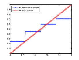
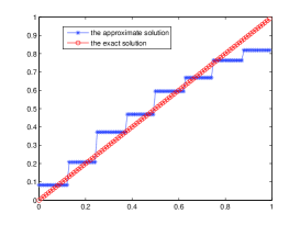
${\delta}=5\%$, $m_{n_{\delta}}=2$	${\delta}=1\%$, $m_{n_{\delta}}=3$
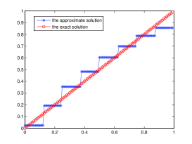
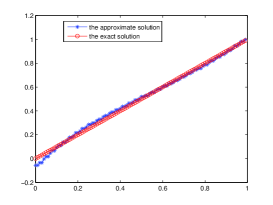
${\delta}=.5\%$, $m_{n_{\delta}}=3$	${\delta}=.05\%$, $m_{n_{\delta}}=5$

Figure 1: Reconstruction of the exact solution $u(t)=t$ using the proposed iterative scheme

We compare the results of the proposed iterative scheme with the iterative scheme proposed in [2]:

$$u_{n}^{\delta}=qu_{n-1}^{\delta}+(1-q)T_{a_{n}}^{-1}K^{*}f_{\delta},\quad u_{0}=0,\quad a_{n}=\alpha_{0}q^{n},\ \alpha_{0}>0.$$ (135)

In this iterative scheme we need to solve the following equation:

$$(a_{n}I+A)z=A^{*}f_{\delta},$$ (136)

where

$$(A)_{i,j}:=\int_{0}^{1}\Phi_{i}(s)\int_{0}^{1}e^{-st}\Phi_{j}(t)dtds,\quad i,j=1,2,\ldots,2^{m},$$ (137)

$$(f_{\delta})_{i}:=\int_{0}^{1}f_{\delta}(s)\Phi_{i}(s)ds,\quad i=1,2,\ldots,2^{m},$$ (138)

and $\Phi_{i}(x)$ are the Haar basis functions. In all the experiments the value of the parameter $m$ in (137) and (138) is $4$, so the size of the matrix $A$ in (136) is fixed to $16\times 16$ at each iteration. The reconstructions obtained by iterative solution (135) are shown in Figure 2.

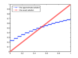
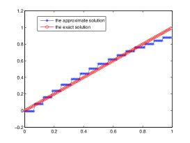
${\delta}=5\%$, $m=4$	${\delta}=1\%$, $m=4$
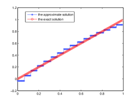
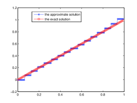
${\delta}=.5\%$, $m=4$	${\delta}=.05\%$, $m=4$

Figure 2: Reconstruction of the exact solution $u(t)=t$ using iterative scheme (135)

In Table 1 we compare the results of the proposed iterative scheme with of iterative scheme (135). Here the proposed iterative and iterative scheme (135) are denoted by $It_{1}$ and $It_{2}$, respectively. For the levels of noise $5\%,$ $1\%$, $0.5\%$ the CPU time of iterative scheme (135) are larger than of these for the proposed iterative scheme, since at each iteration of iterative scheme (135) one needs to solve linear algebraic system (136) with the matrix $A$ of the size $16\times 16$ while in the proposed iterative scheme one only needs to use smaller sizes of the matrix $A$ at each iteration. In general the average errors of the proposed iterative scheme are comparable to of these for iterative scheme (135).

Table 1: fixed vs adaptive iterative scheme

	$It_{1}$			$It_{2}$
${\delta}$	$Avg$	$m_{n_{\delta}}$	CPU time	$Avg$	$m$	CPUtime
			(seconds)			(seconds)
$5\%$	$0.1095$	$2$	$0.1563$	$0.1346$	$4$	$0.5313$
$1\%$	$0.0513$	$3$	$0.2188$	$0.0339$	$4$	$0.5313$
$0.5\%$	$0.0452$	$3$	$0.2344$	$0.0300$	$4$	$0.5469$
$0.05\%$	$0.0250$	$5$	$0.8281$	$0.0206$	$4$	$0.5313$

5 Conclusion

A stopping rule with the parameters $m_{n}$ depending on the regularization parameters $a_{n}$ is proposed. The $m_{n}$ is an increasing sequence of the regularization parameter $a_{n}$. This allows one to start by solving a small size linear algebraic system (129), and one increases the size of the linear algebraic systems only if $G_{n}>C{\delta}^{\varepsilon}.$ In the numerical example it is demonstrated that a simple quadrature method, compound Simpson’s quadrature, can be used for approximating the kernel $g(x,z)$, defined in (8). Our method yields convergence of the approximate solution $u_{n,m_{\delta}}^{\delta}$ to the minimal norm solution of (1). Numerical experiments show that all the average errors of the proposed method are comparable to of these for iterative scheme (135). Our numerical experiments demonstrate that the adaptive choice of the parameter $m_{n}$ is more efficient, in the following sense: the value of the parameters $m_{n}$ of the proposed iterative scheme at the noise levels $5\%$,$1\%$ and $0.5\%$ are smaller than of the parameter $m$, used in the iterative scheme (135). Therefore the computational time of the proposed method at these levels of noise is smaller than the computational time for the iterative scheme (135). The adaptive choice of the parameters $m_{n}$ may give a large size of the matrix $A_{m_{n}}$ in (129), since $m_{n}$ is a non-decreasing sequence depending on the geometric sequence $a_{n}$, so the CPU time increases as the value of the parameter $m_{n}$ increases. In the iterative scheme (135) the size of the matrix $A$ in (136) is fixed at each iteration, so the CPU time depends on the number of iterations. The drawback of using a fixed size $2^{m}\times 2^{m}$ of the matrix $A$ in (136) at each iteration is: the solution $u_{n}^{\delta}$, defined by formula (135), where $n=n({\delta})$ is found by the stopping rule (73) with $m_{n}=m$ $\forall n$, may approximate the minimal norm solution on the finite-dimensional space $L_{m}=\text{span}\{\Phi_{1},\Phi_{2},\ldots,\Phi_{2^{m}}\}$ not accurately, so that for some levels of the noise the exact solution to problem (107) will not be well approximated by any function from $L_{m}$. From Table 1 one can see that the number of basis functions used for an approximation of the minimal norm solution with the accuracy 0.1095 by the iterative scheme with the adaptive choice of $m_{n}$ is four times smaller than the number of these functions used in the iterative scheme with a fixed $m$, while the accuracy is 0.1095 in $It_{1}$ and $0.1346$ in $It_{2}$ (see line 1 in Table 1).

References

[1] P.J. Davis and P. Rabinowitz, Methods of numerical
integration, Academic Press, INC., London, 1984.
[2] S.W. Indratno and A.G. Ramm, Dynamical Systems
Method for solving ill-conditioned linear algebraic systems, Int.
Journal of Computing Science and Mathematics, (to appear).
[3] V. Ivanov,
V. Vasin, V. Tanana, Theory of linear inverse and ill-posed
problems and its applications, VSP, Utrecht, 2002.
[4] V.
Morozov, Methods of solving incorrectly posed problems,
Springer Verlag, New York, 1984.
[5]
A. G. Ramm, Inverse problems, Springer, New York, 2005.
[6]
A. G. Ramm, Dynamical systems method for solving operator equations,
Elsevier, Amsterdam, 2007.
[7]
A. G. Ramm, Discrepancy principle for DSM, I, Comm. Nonlin. Sci. and
Numer. Simulation, 10, N1, 95-101, 2005.
[8]
A. G. Ramm, Discrepancy principle for DSM II, Comm. Nonlin. Sci. and
Numer. Simulation, 13, 1256-1263, 2008.
[9] I. M. Sobol, Multidimensional Quadrature Formulas
and Haar Functions, Nauka, Moscow, 1969.