Non-universal lower bound for the shear viscosity to entropy density ratio

Abstract

The lower bound of the shear viscosity to entropy density ratio is examined using an exact representation of the ratio through the density of states. It is shown that the lower bound in a generic physical system is not universal, its value is determined by the entropy density. Some examples of physical systems are discussed in the paper where one can expect violation of the conformal $1/4\pi$ value.

I Introduction

Experimental evidence from RHIC Adler et al. (2003); Adams et al. (2004) suggests Shuryak (2004); Teaney (2003) that the QCD matter near the (would-be) critical temperature is very close to an ideal fluid, the shear viscosity to entropy density ratio is $\eta/s<0.2$ Romatschke and Romatschke (2007); Heinz and Song (2008). Such small values suggest very strong interactions, and it is therefore a big theoretical challenge to explain the actual $\eta/s$ in this system. Direct calculations with weak coupling resummed perturbation theory in various models Jeon (1995); Wang and Heinz (2003); Aarts and Martinez Resco (2005); Huot et al. (2007); Gagnon and Jeon (2007) and resummations with Boltzmann-equations Jeon and Yaffe (1996); Arnold et al. (2003) suffer generally from the problem that the unperturbed system, ie. the free gas has infinite viscosity, and so small perturbations necessarily remain in the large viscosity regime. This is reflected in the result $\eta/s\sim 1/(g^{4}\log g)$ which is large if the coupling is small. At stronger coupling subleading corrections may alter this result: for example the inclusion of $2-3$ Bremsstrahlung processes into the Boltzmann equation results in a significant difference near the critical region of QCD Xu and Greiner (2008); Xu et al. (2008).

Since perturbation theory is not well controlled in the strong coupling regime, one has to look for alternative methods. A potentially exact method is lattice Monte Carlo simulations. However the actual measurement of the transport coefficients is plagued by the necessity of analytic continuation from imaginary to real time based on a discrete set of data. The inversion of the integral equation for the analytic continuation then has very little sensitivity to the important infrared physics Petreczky (2008). Therefore existing MC results Meyer (2007) depend on not fully controlled assumptions.

A completely different strategy is when one uses a dual description of the theory, where the strong coupling limit is mapped to the small coupling limit of the dual theory. In case of QCD-like theories this is possible only with a much larger symmetry group, the ${\cal N}=4$ SYM theories, where supersymmetry together with the holographic principle makes possible to work, at large $N_{c}$ and large t’Hooft coupling, in a five dimensional gravity with AdS metric Aharony et al. (2000). There the shear viscosity of the conformal field theory can be calculated from graviton absorption Kovtun et al. (2005), resulting in the celebrated $1/4\pi$. In a large class of AdS models this seems to be a lower bound Myers et al. (2009); Myers and Wapler (2008).

Although ${\cal N}=4$ SYM is not QCD, one can argue independently that there is a lower bound in QCD itself Danielewicz and Gyulassy (1985). Then the value of this lower bound may come universally from the large $N_{c}$ large t’Hooft coupling supersymmetric case Kovtun et al. (2005).

The statement that $1/4\pi$ would be the lower bound in any system for the $\eta/s$ ratio is, however, not really proven, only argued for, and it is supported by the fact that we never encountered systems where this bound was violated. But the argumentation has weak points, which suggest that it is not so general as it is commonly believed. First, in the gravity side one can find higher curvature AdS models, where this conclusion fails Kats and Petrov (2009); Buchel et al. (2009); Cai et al. (2009). In the framework of nonrelativistic gases one can also construct counterexamples Cohen (2007); Cherman et al. (2008). Although these examples may describe metastable states Son (2008), but the question of the applicability range of the result is not answered reassuringly.

More importantly, the argumentation is strongly based on the quasiparticle picture. The generic argumentation says Kovtun et al. (2005) that $\eta/s\sim E\tau$ where $E$ is the energy of an excitation, $\tau$ is the lifetime, and uncertainty principle states that $E\tau\mathrel{\hbox to0.0pt{\lower 4.0pt\hbox{\hskip 1.0pt$\sim$}\hss}\raise 1.0pt\hbox{$>$}}\hbar$ which yields $\eta/s\mathrel{\hbox to0.0pt{\lower 4.0pt\hbox{\hskip 1.0pt$\sim$}\hss}\raise 1.0pt\hbox{$>$}}\hbar$. But uncertainty principle, in fact, states that the uncertainty of the energy measurement is related to the lifetime, not the energy value itself. In quasiparticle picture the uncertainty cannot be larger than the energy value itself, but in a generic theory this may not be the case. So, in fact the restriction $E\tau\mathrel{\hbox to0.0pt{\lower 4.0pt\hbox{\hskip 1.0pt$\sim$}\hss}\raise 1.0pt\hbox{$>$}}\hbar$ is not a law of nature, but rather the applicability range of the quasiparticle picture. If the small width quasiparticle approximation cannot be applied, then we have no real arguments in favor of the lower bound. Recently in Noronha-Hostler et al. (2009) the authors have shown that the presence of a continuum in the particle spectrum has important effect on the shear viscosity to entropy density ratio.

To clarify these issues one would need exact statements about the lower limit of $\eta/s$ in physical systems. This is what is attempted in this work, using first principles. For the derivation we have to make some assumptions about some current matrix elements, then one can show that if the transport is dominated by a finite number of quantum channels (ie. there are no large number of particle species) then at finite entropy density the $\eta/s$ ratio has a lower bound. This lower bound, however, depends on the entropy itself; for small entropy density case it is

$$\frac{\eta}{s}\biggr{|}_{\mathrm{min}}\sim\frac{1}{N_{Q}}\,\frac{s}{T^{3}}\,\frac{1}{LT},$$ (1)

where $N_{Q}$ is the number of dominant quantum channels, $L$ is the “interaction range”. This latter can be defined so that parts of the system separated more than $L$ do not interact, or interact weakly; in other words in systems larger than $L$ the entropy is an extensive quantity. For more details and for general $s$ formulae see Section III and (46).

The mathematical reason why $\eta_{min}\sim s^{2}$ depends qualitatively on the fact that, as it will be explained in the paper in detail, the transport coefficients come from integrals depending quadratically on the energy density of states $\varrho$, while the entropy density, for low values of $s$, depends linearly on $\varrho$. Since these integrals have positive kernels, we can treat them as some averaging. So, up to normalization factors $\eta\sim\left\langle{\varrho^{2}}\right\rangle$ and $s\sim\left\langle{\varrho}\right\rangle$. This implies that with this normalization $\eta\geq s^{2}$, and the minimum is therefore proportional to $s^{2}$.

In a finite degree of freedom quasiparticle system the entropy density is proportional to $T^{3}$ and the interactions are screened at most at a scale of the temperature, and so the right hand side is constant. The value of this constant cannot be determined from a general argumentation, but by the argumentation of Danielewicz and Gyulassy (1985); Kovtun et al. (2005) it may be $1/4\pi$. But as a mathematical statement we can claim that there is no lower bound for the shear viscosity to entropy density ratio.

The above formula also tells us where can we expect to have small $\eta/s$ ratio: if the number of dominant quantum channels is large (cf. Cohen (2007); Cherman et al. (2008)), if the system interacts on very large scales (ie. large width systems, where the width is not connected to the temperature), or if we are at low temperatures and the entropy density vanishes faster than $T^{3}$.

In the paper we discuss some systems, where possibly violations of the $1/4\pi$ value are present. These are systems with strong wave function renormalization, large width finite temperature systems and low temperature non-quasiparticle systems. All of these cases can appear in real systems: strong wave function renormalization shows up in strongly coupled quasiparticle systems; at finite temperature QCD we expect large width systems Peshier and Cassing (2005). Finally in systems where there are zero mass excitations, the spectral function must not have a separated Dirac-delta peak even at zero temperature.

The structure of the paper is the following. We first derive exact expressions for the Kubo formula and for the entropy (Section II) through the density of states. In Section III we study the mathematical structure of the $\eta/s$ ratio and determine its minimum. Next we study the quasiparticle-like systems and discuss the small-width quasiparticle case in Section IV. In Section V we examine different situations where the excitations are not small-width quasiparticles, and discuss the impact of the off-shell effects on transport. We finish with conclusions in Section VI.

II The current-current correlator and the entropy density

In this section we derive exact representations for the Kubo formula and the entropy density using the density of states (or energy spectral functions).

II.1 Kubo formula

The shear viscosity, the linear response coefficient for the transversal momentum difference in a plasma, is defined through the Kubo formula in the framework of quantum field theory. We introduce

$$C(x)=\left\langle{[\pi_{xz}(x),\pi_{xz}(0)]}\right\rangle,\qquad\pi_{ij}=T_{ij}-\frac{1}{3}\delta_{ij}T_{\ell}^{\ell},\qquad i,j=1,2,3$$ (2)

where $T$ is the energy-momentum tensor of the system, and the expectation value has to be taken in the equilibrium system:

$$\langle{\hat{Q}}\rangle=\frac{1}{\cal Z}\mathop{\textrm{Tr}}e^{-\beta H}\hat{Q},\qquad{\cal Z}=\mathop{\textrm{Tr}}e^{-\beta H}.$$ (3)

The viscosity is obtained after Fourier transformation as

$$\eta=\lim\limits_{p_{0}\to 0}\frac{C(p_{0},{\bf p}=0)}{p_{0}}.$$ (4)

This discussion can be generalized by using instead of $\pi_{ij}$ a general conserved current $J_{i}$, and look at the linear response function

$$C_{J}(x)=\left\langle{[J_{i}(x),J_{i}(0)]}\right\rangle,$$ (5)

(there is no summation on indices $i$). Because of rotational invariance of the equilibrium system, only the diagonal elements are nonzero here. The corresponding transport coefficient will be called $\eta_{J}$.

We continue by inserting energy eigenstates into the expectation value above.

$$C_{J}(x) =\frac{1}{\cal Z}\sum_{n,m}\biggl{\{}\left\langle{n|e^{-\beta H}J_{i}(x)|m}\right\rangle\left\langle{m|J_{i}(0)|n}\right\rangle-\left\langle{m|e^{-\beta H}J_{i}(0)|n}\right\rangle\left\langle{n|J_{i}(x)|m}\right\rangle\biggr{\}}=$$ (6)

$$=\frac{1}{\cal Z}\sum_{n,m}\left(e^{-\beta E_{n}}-e^{-\beta E_{m}}\right)\,\left\langle{n|J_{i}(x)|m}\right\rangle\left\langle{m|J_{i}(0)|n}\right\rangle.$$

The possible states in the system is characterized by their total energy $k_{0}$ total momentum ${\bf k}$ and other quantum numbers ${\cal K}$

$$\left|{n}\right\rangle=\left|{k_{0},{\bf k},{\cal K}}\right\rangle.$$ (7)

Similarly we denote $\left|{m}\right\rangle=\left|{q_{0},{\bf q},{\cal Q}}\right\rangle$. We will also use the four-momentum notation $k=(k_{0},{\bf k})$ and $q=(q_{0},q)$.

In a realistic quantum field theory the allowed energy eigenvalues can form a continuum, and at finite temperature this is always the case. Therefore it is more adequate to write the sum over the energy in the above expression as an integral over a spectral density. In finite volume spatial momenta form a discrete set, but at larger volumes a continuum representation is applicable for them, while other quantum numbers remain discrete:

$${\bf 1}=\sum_{n}\left|{n}\right\rangle\left\langle{n}\right|=\sum_{{\bf k},{\cal K}}{\int\!\frac{dk_{0}}{2\pi}\,}\,\varrho_{\cal K}(k)\;\left|{k,{\cal K}}\right\rangle\left\langle{k,{\cal K}}\right|=V\sum_{\cal K}{\int\!\frac{d^{4}k}{(2\pi)^{4}}\,}\,\varrho_{\cal K}(k)\;\left|{k,{\cal K}}\right\rangle\left\langle{k,{\cal K}}\right|.$$ (8)

Since the state $\left|{k,{\cal K}}\right\rangle$ is dimensionless in our normalization, therefore $\varrho$ has the dimension of inverse energy. With the energy density of states we can write

$$C_{J}(x)=\frac{V^{2}}{\cal Z}\sum_{\cal K}{\int\!\frac{d^{4}k}{(2\pi)^{4}}\,}\varrho_{\cal K}(k)\sum_{\cal Q}{\int\!\frac{d^{4}q}{(2\pi)^{4}}\,}\varrho_{\cal Q}(q)\,\left(e^{-\beta k_{0}}-e^{-\beta q_{0}}\right)\left\langle{k,{\cal K}|J_{i}(x)|q,{\cal Q}}\right\rangle\left\langle{q,{\cal Q}|J_{i}(0)|k,{\cal K}}\right\rangle.$$ (9)

Using the generator of the space-time translation we write

$$\left\langle{k,{\cal K}|J_{i}(x)|q,{\cal Q}}\right\rangle=e^{i(k-q)x}\left\langle{k,{\cal K}|J_{i}(0)|q,{\cal Q}}\right\rangle,$$ (10)

then the Fourier transformation yields

$$C_{J}(p)=\frac{V^{2}}{\cal Z}\sum_{\cal K}{\int\!\frac{d^{4}k}{(2\pi)^{4}}\,}\varrho_{\cal K}(k)\sum_{\cal Q}{\int\!\frac{d^{4}q}{(2\pi)^{4}}\,}\varrho_{\cal Q}(q)\,(2\pi)^{4}\delta^{(4)}(k-q+p)\,\left(e^{-\beta k_{0}}-e^{-\beta q_{0}}\right)|\left\langle{k,{\cal K}|J_{i}(0)|q,{\cal Q}}\right\rangle|^{2}.$$ (11)

Then the transport coefficient reads

$$\eta_{J}=\beta\,\frac{V^{2}}{\cal Z}\sum_{{\cal K},{\cal Q}}{\int\!\frac{d^{4}k}{(2\pi)^{4}}\,}\varrho_{\cal K}(k)\,\varrho_{\cal Q}(k)e^{-\beta k_{0}}|\left\langle{k,{\cal K}|J_{i}|k,{\cal Q}}\right\rangle|^{2}.$$ (12)

Since $J_{i}$ cannot change the quantum channel without making any change in both energy and momentum, so nonzero result comes only from ${\cal K}={\cal Q}$:

$$\eta_{J}=\beta\,\frac{V^{2}}{\cal Z}\sum_{\cal K}{\int\!\frac{d^{4}k}{(2\pi)^{4}}\,}\varrho_{\cal K}^{2}(k)\,e^{-\beta k_{0}}|\left\langle{k,{\cal K}|J_{i}|k,{\cal K}}\right\rangle|^{2}.$$ (13)

The (temperature-independent) matrix element of $J_{i}$ can be calculated in the free theory with the result

$$\left\langle{k|J_{i}|k}\right\rangle_{0}=q\frac{k_{i}}{k_{0}V}$$ (14)

where $q$ is the charge carried by the current. In case of the energy momentum tensor $q=k_{j}$:

$$\left\langle{k|T_{xz}|k}\right\rangle_{0}=\frac{k_{x}k_{z}}{Vk_{0}}.$$ (15)

In general, we expect an expression of similar structure, since the external momentum carries the Lorentz index of the current, and by dimensional reasons it must be divided by an energy-like quantity. There can still be a Lorentz-invariant factor:

$$\left\langle{k,{\cal K}|J_{i}|k,{\cal K}}\right\rangle=q\frac{k_{i}}{k_{0}V}{\cal J}_{\cal K}(k^{2}),\qquad\mathrm{or}\quad\left\langle{k,{\cal K}|T_{xz}|k,{\cal K}}\right\rangle=\frac{k_{x}k_{z}}{Vk_{0}}\,{\cal T}_{\cal K}(k^{2}).$$ (16)

The reduced current matrix element ${\cal J}_{\cal K}$ depends on the system under consideration, and we cannot tell much more on a generic ground. We will assume, however, that ${\cal J}_{\cal K}$ does not grow at large $k_{0}$ exponentially.

Since the only directional dependence is in the current, we can average angular dependence using (16). Since $\overline{\cos^{2}\theta}=1/3$ and $\overline{\sin^{2}\theta\cos^{2}\theta\cos^{2}\phi}=1/15$, we can write

$$\eta_{J}=\frac{\beta}{3\cal Z}\sum_{\cal K}{\int\!\frac{d^{4}k}{(2\pi)^{4}}\,}\,\frac{{\bf k}^{2}}{k_{0}^{2}}\,e^{-\beta k_{0}}\,({\cal J}_{\cal K}(k)\varrho_{\cal K}(k))^{2},$$ (17)

and for the shear viscosity

$$\eta=\frac{\beta}{15\cal Z}\sum_{\cal K}{\int\!\frac{d^{4}k}{(2\pi)^{4}}\,}\,\frac{({\bf k}^{2})^{2}}{k_{0}^{2}}\,e^{-\beta k_{0}}\,({\cal T}_{\cal K}(k)\varrho_{\cal K}(k))^{2}.$$ (18)

The volume dependence canceled, and so we interpret these formulae as infinite volume limit results.

II.2 The entropy

To calculate the entropy density we start by computing the free energy as

$${\cal Z}=e^{-\beta F}=\mathop{\textrm{Tr}}e^{-\beta H}=\sum_{n}e^{-\beta E_{n}}=\sum_{{\bf k},{\cal K}}{\int\!\frac{dk_{0}}{2\pi}\,}\varrho_{\cal K}(k)e^{-\beta k_{0}}=V\sum_{\cal K}{\int\!\frac{d^{4}k}{(2\pi)^{4}}\,}\varrho_{\cal K}(k)e^{-\beta k_{0}}.$$ (19)

In a strongly coupled system the volume dependence of the free energy can be arbitrary. When we increase the linear size of the system, after a certain scale $L$ one can observe more and more accurately the the linear volume dependence, ie. the free energy becomes an extensive quantity. That means that adjacent volume elements larger than $L$ interact (mostly) with surface interaction, while smaller volume elements interact through the total volume. Therefore this “interaction range” serves also as an infrared cutoff for the relevant interactions. In quasiparticle systems the interaction range corresponds to the linear size of the cross section, the inverse of free mean path. In general strongly interacting systems have large $L$, weakly interacting ones have small $L$.

This is the scale, beyond which a coarse grained description is sensible Langer (1967, 1969), since only there can one speak about densities of different physical quantities. The free energy in a coarse grained description is dominated by the integral of the free energy density, while the corrections coming from the surface interaction are subleading. Therefore in a microscopic description we should choose the volume size at least $V=L^{3}$ in order to catch all the relevant local physics effects. Therefore we define our free energy density as

$$f=-\frac{T}{L^{3}}\ln\left(L^{3}\sum_{\cal K}{\int\!\frac{d^{4}k}{(2\pi)^{4}}\,}\varrho_{\cal K}(k)\,e^{-\beta k_{0}}\right).$$ (20)

We can separate the ground state (vacuum) contribution, where always $\varrho_{vac}(k_{0})=2\pi\delta(k_{0})$:

$$f=-\frac{T}{L^{3}}\ln\left(1+L^{3}\sum_{\cal K}{\int\!\frac{d^{4}k}{(2\pi)^{4}}\,}\varrho_{\cal K}(k)\,e^{-\beta k_{0}}\right).$$ (21)

From this generic form the entropy density reads

$$s=\frac{1}{L^{3}}\ln\left(1+L^{3}\sum\limits_{\cal K}{\int\!\frac{d^{4}k}{(2\pi)^{4}}\,}\varrho_{\cal K}(k)\,e^{-\beta k_{0}}\right)+\frac{1}{\cal Z}\sum\limits_{\cal K}{\int\!\frac{d^{4}k}{(2\pi)^{4}}\,}\,\beta k_{0}\,\varrho_{\cal K}(k)\,e^{-\beta k_{0}}.$$ (22)

Then the transport coefficient to entropy density ratio reads

$$\frac{\eta_{J}}{s}=\frac{\displaystyle\frac{\beta}{3\cal Z}\sum_{\cal K}{\int\!\frac{d^{4}k}{(2\pi)^{4}}\,}\,\frac{{\bf k}^{2}}{k_{0}^{2}}\,e^{-\beta k_{0}}\,({\cal J}_{\cal K}(k)\varrho_{\cal K}(k))^{2}}{\displaystyle\frac{1}{L^{3}}\ln\left(1+L^{3}\sum\limits_{\cal K}{\int\!\frac{d^{4}k}{(2\pi)^{4}}\,}\varrho_{\cal K}(k)\,e^{-\beta k_{0}}\right)+\frac{1}{\cal Z}\sum\limits_{\cal K}{\int\!\frac{d^{4}k}{(2\pi)^{4}}\,}\,\beta k_{0}\,\varrho_{\cal K}(k)\,e^{-\beta k_{0}}}.$$ (23)

In case of shear viscosity we have to substitute ${\cal J}^{2}\to{\bf k}^{2}{\cal T}^{2}/5$.

III Minimization of shear viscosity to entropy density ratio

Equation (23) gives the functional dependence of $\eta_{J}/s$ on $\varrho$, and so we can study mathematically the minimum of this ratio by varying $\varrho$. The above formula, however, contains yet the unknown ${\cal J}$ factor. To say something constructive we have to make assumptions on this function: we will assume that it can get at most power law $k_{0}$ contributions in a strongly interacting system. In this case we can perform an analysis to find the lower bound.

There is a simple way to decrease the value of $\eta_{J}/s$: we start with an arbitrary $\varrho$ with finite $\eta_{J}/s$ and make a rescaling $\varrho\to\lambda\varrho$ with $\lambda\to 0$. Then the integrals of $\varrho$ become small, we can make a linearization in $s$ with respect to $\varrho$. Then the numerator is quadratic, the denominator is linear, and so $\eta_{J}/s\to\lambda\eta_{J}/s$, in the $\lambda\to 0$ limit it vanishes.

In a physical system this simple procedure cannot be performed, because we have a sum rule in each quantum channel

$${\int\!\frac{dk_{0}}{2\pi}\,}\varrho_{\cal K}(k_{0},{\bf k})=U_{\cal K}({\bf k}),\quad\forall\,{\cal K},\,{\bf k}.$$ (24)

But this constraint is not really restricting. To understand it we should remark that all $\varrho$ integrals for $\eta_{J}$ and $s$ are weighted by $e^{-\beta k_{0}}$. Therefore $\eta_{J}/s$ is sensitive to the $k_{0}\leq T$ regime, say, the infrared (IR) regime. The sum rule, on the other hand, depends also on $k_{0}\geq T$ regime, the ultraviolet (UV) regime. Therefore we may rescale the IR part of the energy density of states and still maintain the sum rules.

To see this we assume that we can linearize the entropy density in $\varrho$ and try to find the minimal $\eta_{J}$. The generic case we will discuss later. The assumption of linearizability also means that ${\cal Z}\approx 1$. To simplify the notation we introduce

$$\sum\limits_{\cal K}{\int\!\frac{d^{3}{\bf k}}{(2\pi)^{3}}\,}=\int_{Q}.$$ (25)

For the linearized case, in this symbolic notation the transport coefficient and the linearized entropy density read

$$\eta_{J}=\int_{Q}{\int\!\frac{dk_{0}}{2\pi}\,}\alpha_{Q}(k_{0})\varrho^{2}_{Q}(k_{0})e^{-\beta k_{0}},\qquad s=\int_{Q}{\int\!\frac{dk_{0}}{2\pi}\,}\gamma(k_{0})\varrho_{Q}(k_{0})e^{-\beta k_{0}},$$ (26)

where

$$\alpha_{Q}(k_{0})=\frac{\beta{\bf k}^{2}}{3k_{0}^{2}}\,{\cal J}^{2}_{\cal K}(k),\qquad\gamma(k_{0})=1+\beta k_{0}.$$ (27)

We shall minimize $\eta_{J}$ with the constraint (24), and so we apply Lagrange multipliers to each quantum channel. To have a control to the thermodynamics we also fix the entropy density $s$. Then we have to minimize the expression

$$\min\int_{Q}{\int\!\frac{dk_{0}}{2\pi}\,}\bigl{[}\alpha_{Q}(k_{0})\varrho^{2}_{Q}(k_{0})e^{-\beta k_{0}}-2\lambda\gamma(k_{0})\varrho(k_{0})e^{-\beta k_{0}}-2\lambda_{Q}\varrho_{Q}(k_{0})\bigr{]}.$$ (28)

Its solution provides the spectral function

$$\varrho_{Q}(k_{0})=\frac{\lambda\gamma(k_{0})+\lambda_{Q}e^{\beta k_{0}}}{\alpha_{Q}(k_{0})}.$$ (29)

The normalization condition can be satisfied if

$$\lambda_{Q}=\frac{U_{Q}-\lambda X_{1}}{X_{0}},\qquad\lambda=\frac{s-\int_{Q}U_{Q}X_{1}/X_{0}}{\int_{Q}(X_{2}-X_{1}^{2}/X_{0})},$$ (30)

where

$$X_{0}={\int\!\frac{dk_{0}}{2\pi}\,}\frac{e^{\beta k_{0}}}{\alpha_{Q}(k_{0})},\quad X_{1}={\int\!\frac{dk_{0}}{2\pi}\,}\frac{\gamma(k_{0})}{\alpha_{Q}(k_{0})},\quad X_{2}={\int\!\frac{dk_{0}}{2\pi}\,}\frac{\gamma^{2}(k_{0})}{\alpha_{Q}(k_{0})}e^{-\beta k_{0}}.$$ (31)

Then the minimal $\eta_{J}$ reads

$$\eta_{J}=\frac{\displaystyle\left(s-\int_{Q}\frac{U_{Q}X_{1}}{X_{0}}\right)^{2}}{\displaystyle\int_{Q}\left(X_{2}-\frac{X_{1}^{2}}{X_{0}}\right)^{2}}+\int_{Q}\frac{U_{Q}^{2}}{X_{0}}.$$ (32)

The concrete expressions for $X_{i}$ are potentially divergent. To define still the result we have to introduce an energy cutoff $\Lambda_{0}$ into the system. Then the qualitative behavior of the $X_{i}$ quantities, assuming ${\cal J}^{2}(k_{0})\sim k_{0}^{a}$:

$$X_{0}\sim\Lambda_{0}^{2-a}e^{\beta\Lambda_{0}},\qquad X_{1}\sim\Lambda^{4-a},\qquad X_{2}\sim\mathrm{convergent}.$$ (33)

Therefore removing the energy cutoff results in vanishing $X_{1}^{n}/X_{0}$ factors. This is exactly the mathematical appearance of the qualitative analysis in the beginning of the subsection: the sum rule constraints of (24) can be easily satisfied by tuning only the UV part of $\varrho$.

When we remove the UV cutoff what remains is

$$\eta_{J\mathrm{min}}=\frac{s^{2}}{\int_{Q}X_{2}}.$$ (34)

Evaluating the integral in the denominator, for concreteness for shear viscosity where we assume ${\cal J}\sim{\bf k}^{2}$, we obtain

$$\frac{\eta}{s}\biggr{|}_{\mathrm{min}}\sim\frac{s}{N_{Q}LT^{4}},$$ (35)

where $N_{Q}$ is the effective number of quantum channels. This formula is valid for small $s$.

We remark here that the same line of thought leads to the conclusion that also $\eta/\varepsilon$ has a lower limit which is proportional to $\varepsilon$ itself. Therefore $s$ has no singled out role in this analysis.

We can perform the same analysis for large $s$, too. This time we omit the sum rule constraints, but we cannot omit ${\cal Z}$. Our strategy will be to fix ${\cal Z}s$ and minimize ${\cal Z}\eta_{J}$. Therefore we have to minimize the expression

$$\min\left[\int_{Q}{\int\!\frac{dk_{0}}{2\pi}\,}\alpha_{Q}(k_{0})\varrho_{Q}^{2}(k_{0})e^{-\beta k_{0}}-2\lambda\left(\frac{{\cal Z}\ln{\cal Z}}{L^{3}}+\int_{Q}{\int\!\frac{dk_{0}}{2\pi}\,}\beta k_{0}\varrho_{Q}(k_{0})e^{-\beta k_{0}}\right)\right],$$ (36)

where

$${\cal Z}=1+L^{3}\int_{Q}{\int\!\frac{dk_{0}}{2\pi}\,}\varrho_{Q}(k_{0})e^{-\beta k_{0}}.$$ (37)

The minimum condition yields

$$\varrho_{Q}(k_{0})=\lambda\frac{1+\ln{\cal Z}+\beta k_{0}}{\alpha_{Q}(k_{0})}.$$ (38)

If $\ln{\cal Z}\ll 1$ we get back (29), this corresponds to the small $s$ case. Here we follow the opposite limit and assume that ${\cal Z}$ dominates the above expression in the relevant $k_{0}\leq T$ domain:

$$\varrho_{Q}(k_{0})\approx\lambda\frac{\ln{\cal Z}}{\alpha_{Q}(k_{0})}.$$ (39)

With this density of states we can calculate

$${\cal Z}=1+\lambda Y_{0}\ln{\cal Z},\qquad{\cal Z}s=\frac{1}{L^{3}}\left({\cal Z}\ln{\cal Z}+\lambda Y_{1}\ln{\cal Z}\right),$$ (40)

where

$$Y_{0}=L^{3}\int_{Q}{\int\!\frac{dk_{0}}{2\pi}\,}\frac{e^{-\beta k_{0}}}{\alpha_{Q}(k_{0})},\qquad Y_{1}=L^{3}\int_{Q}{\int\!\frac{dk_{0}}{2\pi}\,}\frac{\beta k_{0}e^{-\beta k_{0}}}{\alpha_{Q}(k_{0})}.$$ (41)

For the case of the shear viscosity, assuming ${\cal J}_{Q}\sim{\bf k}^{2}$ we obtain $Y_{1}\sim Y_{0}\sim N_{Q}(LT)^{4}$. For ${\cal J}_{Q}={\bf k}^{2}$ there is a factor of $3$ between them, so we may assume that their values are of similar order of magnitude in general. Then in the expression of ${\cal Z}s$ the first term is proportional to $(\ln{\cal Z})^{2}$, the second only to $\ln{\cal Z}$. Therefore the second term can be omitted, and we find

$${\cal Z}s\approx\frac{{\cal Z}\ln{\cal Z}}{L^{3}}\qquad\Rightarrow\qquad s=\frac{\ln{\cal Z}}{L^{3}}.$$ (42)

Therefore in the large ${\cal Z}s$ regime $s$ and ${\cal Z}$ are not independent. So if we fix a large value for ${\cal Z}s$ it means fixing large value for separately $s$ and ${\cal Z}$. Large ${\cal Z}$ also means that the vacuum contribution can be omitted, and then

$$\lambda=\frac{\cal Z}{Y_{0}\ln{\cal Z}}.$$ (43)

Finally for the transport coefficient we obtain

$$\eta=\frac{\cal Z}{L^{3}Y_{0}},$$ (44)

therefore the $\eta/s$ ratio reads

$$\frac{\eta}{s}\biggr{|}_{\mathrm{min}}=\frac{e^{L^{3}s}}{Y_{0}L^{3}s}\sim\frac{e^{L^{3}s}}{L^{3}s}\frac{1}{N_{Q}(LT)^{4}}.$$ (45)

So we can summarize the small and large $s$ cases in a common formula

$$\frac{\eta}{s}\biggr{|}_{\mathrm{min}}\sim\frac{{\cal F}(L^{3}s)}{N_{Q}(LT)^{4}},$$ (46)

where for small values ${\cal F}(x)\sim x$, for large values ${\cal F}(x)\sim e^{x}/x$.

The results has several interesting consequences. First of all we see that if we distribute the entropy uniformly into $N_{Q}$ quantum channels, we can reduce the $\eta/s$ ratio at any temperature to zero. This corresponds to the construction of Cherman et al. (2008) with large number of particle species. In that model $L^{3}s\sim\ln{N_{Q}}$ because of the mixing entropy, which for large $N_{Q}$ leads to $1/\ln N_{Q}$ dependence for the shear viscosity to entropy ratio. In this construction the entropy goes to infinity, while the shear viscosity stays constant.

If we fix the number of dominant quantum channels then the $\eta/s$ ratio has a minimum for each fixed entropy, but this minimum depends on the value of the entropy itself. The theoretical lower bound is zero, which, however, can be reached only at zero entropy, ie. at zero temperature.

If we have non-interacting quasiparticles, then the effective interaction range is zero, $L\to 0$ and the $\eta/s$ ratio is infinity. In case of weak coupling the interaction range is related to the cross section, or the inverse lifetime of the particle. A more detailed description for the quasiparticle systems is done in the next section.

IV Quasiparticle systems

Apart from the theoretical bound determined above, it is still a question, how the $\eta/s$ ratio behaves in a real system. In this Section we actualize the general formulae for quasiparticle systems, and discuss the small width case.

For quasiparticles we use that the energy contribution from non-interacting subsystems simply added in the free energy, so in weakly interacting bosonic/fermionic system we can write

$$f=T{\int\!\frac{d^{4}k}{(2\pi)^{4}}\,}\,\varrho_{QP}(k)\,(\mp)\ln\left(1\pm e^{-\beta k_{0}}\right).$$ (47)

The entropy density can be calculated as $s=-\partial f/\partial T$.

$$s=\sum\limits_{Q}{\int\!\frac{d^{4}k}{(2\pi)^{4}}\,}\left[\frac{\beta k_{0}}{e^{\beta k_{0}}\pm 1}\pm\ln(1\pm e^{-\beta k_{0}})\right]\varrho_{Q}(k)\equiv\sum\limits_{Q}{\int\!\frac{d^{4}k}{(2\pi)^{4}}\,}{\cal X}(\beta k_{0})\,\varrho_{Q}(k).$$ (48)

For concreteness we will calculate the shear viscosity coefficient from now on. The viscosity to entropy density ratio reads

$$\frac{\eta}{s}=\frac{\displaystyle\frac{\beta}{15\cal Z}\sum_{\cal K}{\int\!\frac{d^{4}k}{(2\pi)^{4}}\,}\,\frac{({\bf k}^{2})^{2}}{k_{0}^{2}}\,e^{-\beta k_{0}}\,({\cal J}_{\cal K}(k)\varrho_{\cal K}(k))^{2}}{\displaystyle\sum\limits_{Q}{\int\!\frac{d^{4}k}{(2\pi)^{4}}\,}{\cal X}(\beta k_{0})\,\varrho_{Q}(k)}.$$ (49)

Formally it is similar to the perturbation theory motivated expressions of Peshier and Cassing (2005). But here the logic is different, we do not use propagating states, but instead energy eigenstates as intermediate states.

To treat the problem analytically we will assume that ${\cal J}_{\cal K}(k)$ does not depend too strongly on the momentum on the relevant momentum regime, where, for example $\varrho(k)$ exhibits a peak. We also will assume that there is a single dominant quantum channel where the largest contribution for entropy as well as the shear viscosity comes. Therefore we analyze a reduced shear viscosity from the dominant quantum channel as

$$\bar{\eta}=\frac{\beta}{15}\,{\int\!\frac{d^{4}k}{(2\pi)^{4}}\,}\,\frac{({\bf k}^{2})^{2}}{k_{0}^{2}}\,e^{-\beta k_{0}}\,\varrho_{\cal K}^{2}(k).$$ (50)

The $\eta/s$ ratio then reads

$$\frac{\bar{\eta}}{s}=\frac{\displaystyle\frac{\beta}{15}{\int\!\frac{d^{4}k}{(2\pi)^{4}}\,}\,\frac{({\bf k}^{2})^{2}}{k_{0}^{2}}\,e^{-\beta k_{0}}\,\varrho^{2}_{\cal K}(k)}{\displaystyle{\int\!\frac{d^{4}k}{(2\pi)^{4}}\,}{\cal X}(\beta k_{0})\,\varrho_{Q}(k)}.$$ (51)

We hope that $\bar{\eta}$ characterizes well the true $\eta/s$, so we will use this quantity to assess the importance of the off-shell effects.

IV.1 Small width approximation

If the integral is dominated by a Dirac-delta-like peak then near the peak region we may approximate

$$\varrho_{\cal K}(k)\biggr{|}_{k_{0}\approx\varepsilon_{k}}\approx\frac{2\Gamma}{(k_{0}-\varepsilon_{k})^{2}+\Gamma^{2}}.$$ (52)

In relativistically invariant systems $\varepsilon_{k}^{2}=k^{2}+m^{2}$, and approximately the same is true at finite temperatures with thermal masses.

The product of two functions can be approximated by

$$\varrho_{\cal K}^{2}(k)\approx\varrho_{\cal K}(k_{0}=\varepsilon_{k})\varrho(k)\approx\frac{2}{\Gamma}\,2\pi\delta(k_{0}-\varepsilon_{k}).$$ (53)

By replacing back this expression into (50) we find

$$\bar{\eta}_{QP}=\frac{1}{15\pi\Gamma T}\int\limits_{0}^{\infty}dk\,\frac{k^{6}}{\varepsilon_{k}^{2}}e^{-\varepsilon_{k}/T},$$ (54)

where the $QP$ subscript refers to the small-width quasiparticle case. Depending on the dispersion relation we can obtain results like

$$\bar{\eta}_{QP}=\left\{\begin{array}[c]{ll}\displaystyle\rule[-10.00002pt]{0.0pt}{10.00002pt}\frac{8}{5\pi^{2}}\frac{T^{4}}{\Gamma},&\mathrm{if}\;\varepsilon_{k}=k\cr\displaystyle\rule[-10.00002pt]{0.0pt}{10.00002pt}\frac{1}{\sqrt{2\pi}}\frac{m^{3/2}T^{5/2}}{\Gamma}\,e^{-m/T},&\mathrm{if}\;\varepsilon_{k}=m+\frac{k^{2}}{2m}\cr\displaystyle\frac{4}{15\sqrt{2\pi}}\frac{m^{7/2}T^{1/2}}{\Gamma},&\mathrm{if}\;\varepsilon_{k}=\frac{k^{2}}{2m}\cr\end{array}\right.$$ (55)

The first case corresponds the high temperature case, the second the low temperature relativistic case, the third a low temperature nonrelativistic gas case (Chapman-Enskog formula).

The free energy in the quasiparticle case (52) reads after partial integration:

$$f_{QP}=-\frac{1}{6\pi^{2}}\int\limits_{E_{0}}^{\infty}\!dE\,k(E)^{3}n(E),$$ (56)

where $n_{\pm}(E)=(e^{\beta E}\pm 1)^{-1}$ Bose-Einstein or Fermi-Dirac particle number density. For the entropy we obtain

$$s=\frac{\beta}{6\pi^{2}}\int\limits_{E_{0}}^{\infty}dE\,n_{\pm}(E)\frac{d}{dE}(Ek^{3}(E)).$$ (57)

In the different dispersion relation case we get:

$$s_{QP}=\left\{\begin{array}[c]{ll}\displaystyle\rule[-10.00002pt]{0.0pt}{10.00002pt}{\cal A}_{\pm}\frac{4T^{3}\pi^{2}}{90},&\mathrm{if}\;\varepsilon_{k}=k\cr\displaystyle\rule[-10.00002pt]{0.0pt}{10.00002pt}\frac{T^{1/2}m^{5/2}}{(2\pi)^{3/2}}e^{-\beta m},&\mathrm{if}\;\varepsilon_{k}=m+\frac{k^{2}}{2m}\cr\displaystyle\frac{(mT)^{3/2}}{2(2\pi)^{3/2}},&\mathrm{if}\;\varepsilon_{k}=\frac{k^{2}}{2m},\cr\end{array}\right.,$$ (58)

where ${\cal A}_{\pm}=(1,8/7)$. Then the ratio reads

$$\frac{\bar{\eta}_{QP}}{s_{QP}}=\left\{\begin{array}[c]{ll}\displaystyle\rule[-10.00002pt]{0.0pt}{10.00002pt}\frac{36}{{\cal A}_{\pm}\pi^{4}}\frac{T}{\Gamma},&\mathrm{if}\;\varepsilon_{k}=k\cr\displaystyle\rule[-10.00002pt]{0.0pt}{10.00002pt}2\pi\,\frac{T^{2}}{\Gamma m},&\mathrm{if}\;\varepsilon_{k}=m+\frac{k^{2}}{2m}\cr\displaystyle\frac{16\pi}{15}\,\frac{m^{2}}{\Gamma T},&\mathrm{if}\;\varepsilon_{k}=\frac{k^{2}}{2m}\cr\end{array}\right.$$ (59)

In the first, $m\ll T$ case the width must determined by the temperature which is the only scale in the system: $\Gamma\sim T$ by dimensional reasons. Therefore in the first case we obtain temperature independent ratio.

In the second, low temperature massive case we have to take into account that the quasiparticles are stable at zero temperature, and the first scattering states which are responsible for the decay have to be excited thermally. Therefore we expect that $\Gamma\sim e^{-M/T}$, where $M$ is the mass of the excited state. In this case the ratio grows like $T^{2}e^{M/T}$ at small temperature.

In the third case the width can be proportional to $T$, but also in this case the ratio will grow like $1/T^{2}$.

So we can see that in the quasiparticle case the $\eta/s$ ratio is at most constant, but in all massive cases it is bounded from below. The lower bound of this ratio is probably provided by the AdS/CFT results.

The inverse proportionality to $\Gamma$ also suggests that in environments where the correlation lengths, in particular the quasiparticle lifetimes grow, the $\eta/s$ ratio will decrease. This is the case for second order phase transitions.

V Relevance of the off-shell effects in different physical situations

In the field theoretical systems besides the (quasi)particles one should count with a multiparticle contribution which appears as a continuum in the energy density of states. The simple picture suggested by the small width quasiparticle approximation of the previous subsection may break down more or less in case of strong continuum.

In this section we consider three physical situations where the presence of off-shell effects can significantly modify the small width quasiparticle picture. The first is the effect of the wave function renormalization, the second is the case of large thermal width, the third is the case of a theory with zero mass excitations.

V.1 Wave function renormalization

As a first example we take a system where besides the quasiparticle peak there is a separate continuum. The normalization requirement (24) tells us that in the full case the peak should be smaller than in the quasiparticle approximation: the factor we have to apply is the wave function renormalization. At small enough temperatures we will see only the quasiparticle peak, then the $\eta/s$ ratio is simply rescaled by the wave function renormalization factor.

To demonstrate the effect we take a toy model, where the full spectral density is taken as

$$\varrho(k)=Z\varrho_{QP}(k)+2\pi\frac{1-Z}{E_{2}-E_{1}}\Theta(E_{2}>k_{0}>E_{1}),$$ (60)

ie. we take a step-function-like spectral density in the continuum regime, which means that in this toy model we do not care about the details of the continuum, only an effective height is taken into account. Here we take the relativistic form $E_{1,2}^{2}={\bf k}^{2}+M_{1,2}^{2}$, while $\varrho_{QP}$ has the form of (52). The proportionality factors are taken into account to satisfy the sum rule

$${\int\!\frac{dk_{0}}{2\pi}\,}\varrho(k_{0})={\int\!\frac{dk_{0}}{2\pi}\,}\varrho_{QP}(k_{0})=1.$$ (61)

We will assume the hierarchy $m\ll M_{1,2}$ and $T<M_{1}$. In this limit in the square $\varrho^{2}$ we can neglect the cross terms, and we can use nonrelativistic approximation in the $E_{1,2}$ energies. What we obtain in the leading order

$$\bar{\eta}=Z^{2}\bar{\eta}_{QP}+\frac{1}{5\sqrt{2\pi}}\,\frac{(1-Z)^{2}T^{5/2}M_{1}^{5/2}}{\Delta M^{2}}\,e^{-M_{1}/T},$$ (62)

where $\Delta M=M_{2}-M_{1}$. With similar assumptions the entropy density reads:

$$s=Zs_{QP}+\frac{1}{(2\pi)^{3/2}}\frac{(1-Z)T^{3/2}M_{1}^{5/2}}{\Delta M}\,e^{-M_{1}/T}.$$ (63)

If the temperature is lower than the threshold, then the radiative corrections for both $\bar{\eta}$ and $s$ are suppressed. Then approximately we obtain

$$\frac{\bar{\eta}}{s}=Z\,\frac{\bar{\eta}_{QP}}{s_{QP}}.$$ (64)

That means that even though the continuum contribution cannot be seen, its effect is measurable in the $\eta/s$ ratio.

The value of $Z$ is determined by the relative contribution of the continuum in the sum rule as compared to the quasiparticle peak. In weak coupling cases this ratio is suppressed by (powers of) the coupling constant, so $Z\approx 1$ and so the effect on $\eta/s$ is small. However, in strongly coupled theories the continuum becomes more and more important, and, correspondingly, the wave function decreases. As $Z\to 0$ the continuum contribution slowly takes over and it will dominate the $\eta/s$ ratio. In this simple case the theoretical $Z\to 0$ limit the continuum yields $\bar{\eta}/s\sim T/\Delta M$. This demonstrates a mathematical example where in a constructed system the $\eta/s$ ratio can go to zero. Still, we have to remark that there does not exist a physical system where this type of continuum would be manifested. But it emphasizes the importance of the continuum part of the spectral function in the transport. Two more realistic cases will be studied in the next subsections.

V.2 Large width case

In lots of realistic examples there is a quasiparticle peak, but its width is large, comparable to the mass scales of the system, cf. for example Peshier and Cassing (2005). At finite temperature strongly coupled theories, moreover, the quasiparticle peak can merge with the continuum, forming a broad, slowly varying spectral function, as it can be seen for example in the 2PI simulations Arrizabalaga and Reinosa (2007a); Jakovac (2007); Arrizabalaga and Reinosa (2007b). In this case the “width” of the peak has nothing to do with the quasiparticles. In fact there are no real particles in the plasma, the excitations decay before a particle is formed. Correspondingly, as the width grows, the quasiparticle picture becomes less and less good approximation.

To treat this effect numerically in the case of the transport coefficients, we take a spectral function which could describe a spectral function of a quantum channel at finite temperature, and which is of a Breit-Wigner-type form

$$\varrho_{BW}(k)=\frac{1}{\cal N}\frac{4\gamma_{k}^{2}k_{0}}{(k_{0}^{2}-E_{k}^{2})^{2}+\gamma_{k}^{4}}.$$ (65)

The ${\cal N}$ prefactor is necessary for normalization, is ${\cal N}=(\pi+2\arctan(E_{k}^{2}/\gamma_{k}^{2}))/(2\pi)$. In the above formula the dispersion relation and the momentum dependence of the $\gamma$ parameter is arbitrary, but we assume spatial rotational invariance. In the weak coupling limit the width corresponds to $\Gamma=\gamma^{2}/(2E_{k})$. In the high temperature field theories we expect $\gamma\sim g^{2}T$. In strongly coupled case $\gamma\gg T$ is also possible.

In the $\bar{\eta}/s$ formula we rescale by the temperature, so we choose $T=1$. Then we have to calculate

$$\frac{\bar{\eta}}{s}=\frac{\displaystyle\int\limits_{0}^{\infty}dk\,k^{6}\int\limits_{0}^{\infty}dk_{0}\,e^{-k_{0}}\,(\varrho_{BW}/k_{0})^{2}}{\displaystyle 15\int\limits_{0}^{\infty}dk\,k^{2}\int\limits_{0}^{\infty}dk_{0}\,\left(k_{0}(e^{k_{0}}-1)^{-1}-\ln(1-e^{-k_{0}})\right)\varrho_{BW}},$$ (66)

where we have chosen, for the sake of concreteness, the minus sign in ${\cal X}$.

For a particular choice of $\gamma_{k}=\gamma=\mathrm{const}$ and $E_{k}=\sqrt{k^{2}+m^{2}}$ we find the plot of the ratio in Fig. 1.

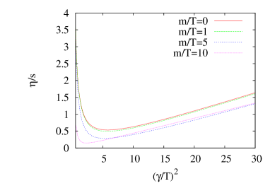
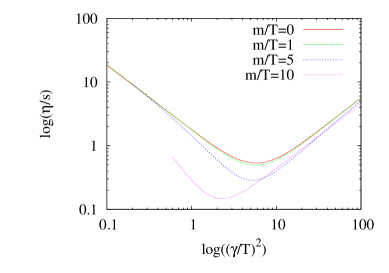
Figure 1: The shear viscosity to entropy ratio as a function of the imaginary self energy.

This figure shows how the small width quasiparticle picture which yields in this case $\sim T^{2}/\gamma^{2}$ breaks down for larger width case, where we find $\sim\gamma^{2}/T^{2}$ behavior. Looking at these figures as function of temperature at fixed $\gamma$ we see that at high temperatures the $\eta/s$ ratio increases with increasing temperature, while at low temperature it decreases with increasing temperature. While the former is characteristic for gases, the latter is the behavior of the fluids. So in this approximation we can give an account for the $\eta/s$ ratio in the fluid-gas crossover.

How can we understand mathematically this behavior? The small width regime corresponds to the quasiparticle approximation above, so we have to understand the large $\gamma$ regime, so examine the $\gamma\gg T$ case. Because of the exponential suppression for $k_{0}$, the value of $k_{0}$ cannot grow larger than $T$. The peak region, however, is in the vicinity of $|k_{0}^{2}-E_{k}^{2}|\sim\gamma^{2}$. Therefore $k_{0}$ cannot play a role in saturating the integrand (unless we are in the quasiparticle regime $\gamma\ll m$), and so we can neglect $k_{0}$ here. Then the dominant contribution should come from $E_{k}\sim\gamma$, since there is no exponential suppression for $k$. As a result $k_{0}\ll k$ and the $k_{0}$ and $k$ integrations decouple. For $\gamma\gg m$ case $E_{k}\sim\gamma\gg m$ means that we can use ultrarelativistic dispersion relation. Then for the numerator we have

$$\bar{\eta}\to\int\limits_{0}^{\infty}dk_{0}\,e^{-k_{0}}\int\limits_{0}^{\infty}dk\,k^{6}\,\frac{1}{{\cal N}^{2}}\frac{16\gamma^{4}}{(k^{4}+\gamma^{4})^{2}}\sim\gamma^{3},$$ (67)

and for the denominator we obtain

$$s\to\int\limits_{0}^{\infty}dk_{0}\,k_{0}\left(k_{0}(e^{k_{0}}-1)^{-1}-\ln(1-e^{-k_{0}})\right)\int\limits_{0}^{\infty}dk\,k^{2}\frac{1}{\cal N}\frac{4\gamma^{2}}{k^{4}+\gamma_{k}^{4}}\sim\gamma.$$ (68)

Therefore we expect that the ratio grows like $\gamma^{2}/T^{2}$. In the opposite case, when $\gamma\ll m$, but the decoupling of the integrals is still true, then we can neglect the $\gamma$ factor in the denominator and we obtain

$$\bar{\eta}\to\int\limits_{0}^{\infty}dk_{0}\,e^{-k_{0}}\int\limits_{0}^{\infty}dk\,k^{6}\,\frac{1}{{\cal N}^{2}}\frac{16\gamma^{4}}{((k^{2}+m^{2})^{2}}\sim\frac{\gamma^{4}}{m^{2}},$$ (69)

and

$$s\to\int\limits_{0}^{\infty}dk_{0}\,k_{0}\left(k_{0}(e^{k_{0}}-1)^{-1}-\ln(1-e^{-k_{0}})\right)\int\limits_{0}^{\infty}dk\,k^{2}\frac{1}{\cal N}\frac{4\gamma^{2}}{(k^{2}+m^{2})^{2}}\sim\frac{\gamma^{2}}{m}.$$ (70)

Therefore the ratio behaves as $\gamma^{2}/m$, so the trend of large $\gamma$ regime continues.

To have a feeling of when does the small-width description start to dominate, we remark that the quasiparticle contribution is at one hand suppressed by $e^{-E_{k}}$, but, on the other hand, the denominator can be small, too. Decoupling of the integrals will not be true if the denominator can compensate the exponential suppression. In the small mass case, when also $\gamma\gg m$ is true, the quasiparticle regime gives $e^{-k}/\gamma^{8}$ with $k\sim\gamma$, as opposed to the $1/4\gamma^{8}$ factorized case. So on-shell effects will become strong if $\gamma\mathrel{\hbox to0.0pt{\lower 4.0pt\hbox{\hskip 1.0pt$\sim$}\hss}\raise 1.0pt\hbox{$<$}}1.4$. In the large mass case the on-shell contribution is $e^{-E_{k}}/\gamma^{8}$ with $E_{k}\sim m$, the off-shell effects yield $1/m^{8}$. Then the borderline is at $\gamma\sim me^{-m/8}$. In the hypothetical $m\to\infty$ case, therefore, there is no quasiparticle regime, the linear $\gamma^{2}$ trend will continue until $\gamma=0$, where the ratio is zero.

V.3 Low temperature systems with zero mass excitation

If we wonder whether we can reach in a real system zero value for $\eta/s$, with finite number of quantum channels, we must reach, according to (46), zero entropy. In a real system can happen only at zero temperature. In the small-width case, as we have seen, the $\eta/s$ ratio diverges in the massive case, and, formally, stay constant in the zero mass case.

The zero mass systems, however, need a more detailed study, since there are never classical Dirac-delta-like spectral functions. To see this, we recall that if we take a quantum field theoretical system with a stable particle with mass $m$ which interacts with another particle with mass $M$ then the spectral function of this system will contain a Dirac-delta peak at $k_{0}=m$ and a continuum starting at the threshold $m+M$. The imaginary part of the self energy, because of kinematical reasons, is proportional to $\sqrt{\lambda(p^{2},m^{2},M^{2})}$, where $\lambda(x,y,z)=(x-y-z)^{2}-4y^{2}z^{2}$. For a finite $M$ this leads to a square-root behavior for the complete spectral function, $\varrho\sim\sqrt{p^{2}-(m+M)^{2}}$ near the threshold.

If the massive particle interacts with a zero mass particle, all this means that there is no gap between the quasiparticle peak and the continuum. Moreover, in this case $\sqrt{\lambda(p^{2},m^{2},0)}=p^{2}-m^{2}$, which is the same as the tree level part of the real part. This has the consequence that near the threshold the spectral function is divergent $\varrho\sim(p^{2}-m^{2})^{-1}$. There are logarithmic corrections to this behavior; for example in QED at one loop level in Lorenz gauge Peshkin and Schroeder (1995)

$$\varrho(p^{2}\approx m^{2})=\frac{\displaystyle 2\Theta(p^{2}-m^{2})\frac{\alpha}{\pi}}{\displaystyle(/p-m)\left(\left(1+\frac{\alpha}{\pi}\ln\left|\frac{p^{2}-m^{2}}{\mu^{2}}\right|\right)^{2}+\frac{\alpha^{2}}{\pi^{2}}\right)}.$$ (71)

The leading logarithmic corrections can be resummed by renormalization group or by Bloch-Nordsieck construction Bogoljubov and Shirkov (1959), the result is the modification of the threshold behavior

$$\varrho(p^{2}\approx m^{2})=\frac{2\Theta(p^{2}-m^{2})(/p+m)m^{-2\beta}\sin\alpha}{(p^{2}-m^{2})^{1-\beta}},\qquad\beta=-\frac{\alpha}{\pi},\;\alpha=\frac{e^{2}}{4\pi}.$$ (72)

The main features, however, still survived: there is no gap between the quasiparticle peak and the continuum, and there is a rising spectral function as we approach the mass shell.

This behavior can be studied numerically, too. In case of QCD one can use Monte Carlo data to reconstruct the spectral function Biro et al. (2007), which exhibits qualitatively the same behavior as in the QED case.

According to the above analysis in all systems containing zero mass particles, the energy density of states cannot contain a zero width quasiparticle. The would-be quasiparticle continuously radiates long-living soft zero mass excitations, and continuously interacts with them. The spectral function is not Lorentzian, it has no “width” in the usual sense, and it does not describe a decay, too. At larger temperature we will still observe a quasiparticle, although the mechanism how it is formed is far from trivial Blaizot and Iancu (1997). At low temperatures, however, we are in a non-quasiparticle system, where the effect of the threshold behavior cannot be neglected.

At small temperatures we are in an almost Lorentz invariant system. Because of the volume normalization we can write $\varrho(k)=k_{0}\bar{\varrho}(k^{2})$, where $\bar{\varrho}$ depends only on the Lorentz invariant $k^{2}$ form. Then we write (cf. (51))

$$\frac{\bar{\eta}}{s}=\frac{\displaystyle\beta{\int\!\frac{d^{4}k}{(2\pi)^{4}}\,}\,({\bf k}^{2})^{2}e^{-\beta k_{0}}\,{\bar{\varrho}}^{2}(k)}{\displaystyle 15{\int\!\frac{d^{4}k}{(2\pi)^{4}}\,}k_{0}{\cal X}(\beta k_{0})e^{-\beta k_{0}}\,\bar{\varrho}(k)}.$$ (73)

The exponential factor forces the system to have the possible lowest energy values, ie. near the threshold.

First let us assume that the lowest lying threshold is at $k^{2}=M^{2}$ with finite mass. This is conceivable if the zero mass particle is not asymptotic state, like in low energy QCD. Near the colorless bound states, which have color multipole moments, the gluons can still exist, and the effective gluon cloud can result in a continuous threshold behavior. In this case we can use $\beta k_{0}>\beta M\gg 1$, and so ${\cal X}(\beta k_{0})\approx\beta k_{0}$. We change into 4D polar-coordinates ($k_{0}=k\cosh\eta,\,k_{z}=k\sinh\eta\cos\theta,\,k_{y}=k\sinh\eta\sin\theta\sin\phi,\,k_{x}=k\sinh\eta\sin\theta\cos\phi$), taking into account that $k_{0}>0$, and the 3D rotational invariance:

$${\int\!\frac{d^{4}k}{(2\pi)^{4}}\,}\Theta(k_{0})\to\frac{1}{4\pi^{3}}\int\limits_{0}^{\infty}dkk^{3}\int\limits_{0}^{\infty}d\eta\sinh^{2}\eta.$$ (74)

We use the integral formula

$$\int\limits_{0}^{\infty}d\eta\sinh^{n}\eta e^{-z\cosh\eta}=\frac{K_{n/2}(z)\Gamma\left(\frac{n+1}{2}\right)}{\sqrt{\pi}\,(z/2)^{n/2}}$$ (75)

($K_{n}$ is the modified Bessel function of the second kind), and the asymptotic form $K_{n}(x)=\sqrt{\pi/(2x)}e^{-x}$ to arrive at:

$$\frac{\bar{\eta}}{s}=\frac{T^{2}\int\limits_{0}^{\infty}dk\,k^{7/2}\,e^{-\beta k}\bar{\varrho}^{2}(k)}{\int\limits_{0}^{\infty}dk\,k^{7/2}\,e^{-\beta k}\bar{\varrho}(k)}$$ (76)

Near the threshold we power expand the spectral function like

$$\bar{\varrho}(k\approx M)={\cal C}\Theta(k-M)\,(k^{2}-M^{2})^{w}.$$ (77)

And then find

$$\frac{\bar{\eta}}{s}=\frac{\Gamma(1+2w)}{\Gamma(1+w)}\,{\cal C}(2M)^{w}\,T^{2+w}.$$ (78)

This result cleanly shows that if there exist a system described above, it must have a vanishing $\eta/s$ ratio in the $T\to 0$ limit.

If the zero mass particle is an asymptotic state, then the lowest lying energy eigenvalues belong to the quantum channel of the massless particle. Since it interacts with itself, the spectral function has no gap here, too. A special class is the conform theories, another the weakly interacting gauge bosons, like the photon gas, where the photon-photon scattering is mediated by virtual electron loop. In the massless case the above analysis goes through without modification and it yields

$$\frac{\bar{\eta}}{s}\sim{\cal C}T^{2(1+w)}.$$ (79)

This result could be obtained by purely dimensional analysis, since the dimension of ${\cal C}$ is $-2(1+w)$. The numerator of (73) contains $\varrho^{2}$, the denominator only $\varrho$, so there remains a factor ${\cal C}$ in the ratio. Since the ratio is dimensionless, something has to compensate this factor. In the massless case, only the temperature can do that: thus we obtain $\sim T^{2(1+w)}$ dependence.

In conformal field theories without anomalous dimensions ${\cal C}$ is dimensionless and $w=-1$. That predicts a temperature-independent $\eta/s$ ratio. In other cases, ie. either in a non-conformal field theory or in a conformal field theory with anomalous dimension $w$ can differ from $-1$, then we again observe a vanishing $\eta/s$ ratio in the zero temperature limit.

VI Conclusion

In this paper we examined the shear viscosity to entropy density ratio using exact representation through the density of states or energy spectral functions. We examined what can be said purely mathematically about the ratio, assuming some physical conditions (sum rules) for the spectral functions, and keeping the entropy density constant. We concluded that the $\eta/s$ ratio has no lower bound in a most generic class of physical systems. To understand this statement qualitatively we recall that $\eta\sim\varrho^{2}$ and $s\sim\varrho$ if the temperature is low enough. Therefore if the density of states exhibits large peaks (quasiparticle systems) then $\varrho^{2}\gg\varrho$ and so the $\eta/s$ ratio is large; if $\varrho$ is small everywhere then $\varrho^{2}\ll\varrho$ and the ratio is small. However, if we fix the entropy density then there is a minimum, where $\eta\sim s^{2}$. This means that $\eta/s$ can go to zero (in a fixed system) only at zero entropy density, ie. at zero temperature.

Although mathematically the situation is clear, it is hard to show physical systems where a small $\eta/s$ ratio can occur. First of all if it consists of quasiparticle at all, they must not have small width, since the small width approximation excludes small $\eta/s$ ratio. Candidates for such a system are quasiparticle systems with strong continuum (small wave function renormalization constant), high temperature strongly interacting systems or low temperature systems with zero mass excitations. In the first two cases it is possible to go below $1/4\pi$, but we can never reach zero value. In the third case if the threshold behavior is $(k^{2}-M^{2})^{w}$ then the $\eta/s$ ratio can reach zero as $T^{2(1+w)}$ (in $M=0$ case) or $T^{2+w}$ (massive case). So if $w>-1$ then we will find a vanishing ratio in the $T\to 0$ limit.

As far as the heavy ion experiments are concerned, the QCD at finite temperature and density represents a finite entropy density system. Therefore there is a lower bound for the $\eta/s$ ratio, but its value is not necessarily $1/4\pi$. However, the relevant scales are set either by $\Lambda_{QCD}$ or the temperature (since the couplings are of order one), and these two scales are again similar. Therefore we are close to a one-scale system, where the predictions of the conformal theory may apply.

References

- Adler et al. (2003) S. S. Adler et al. (PHENIX), Phys. Rev. Lett. 91, 182301 (2003), eprint nucl-ex/0305013.
- Adams et al. (2004) J. Adams et al. (STAR), Phys. Rev. Lett. 92, 052302 (2004), eprint nucl-ex/0306007.
- Shuryak (2004) E. Shuryak, Prog. Part. Nucl. Phys. 53, 273 (2004), eprint hep-ph/0312227.
- Teaney (2003) D. Teaney, Phys. Rev. C68, 034913 (2003), eprint nucl-th/0301099.
- Romatschke and Romatschke (2007) P. Romatschke and U. Romatschke, Phys. Rev. Lett. 99, 172301 (2007), eprint 0706.1522.
- Heinz and Song (2008) U. W. Heinz and H. Song, J. Phys. G35, 104126 (2008), eprint 0806.0352.
- Jeon (1995) S. Jeon, Phys. Rev. D52, 3591 (1995), eprint hep-ph/9409250.
- Wang and Heinz (2003) E. Wang and U. W. Heinz, Phys. Rev. D67, 025022 (2003), eprint hep-th/0201116.
- Aarts and Martinez Resco (2005) G. Aarts and J. M. Martinez Resco, JHEP 03, 074 (2005), eprint hep-ph/0503161.
- Gagnon and Jeon (2007) J.-S. Gagnon and S. Jeon, Phys. Rev. D76, 105019 (2007), eprint 0708.1631.
- Huot et al. (2007) S. C. Huot, S. Jeon, and G. D. Moore, Phys. Rev. Lett. 98, 172303 (2007), eprint hep-ph/0608062.
- Arnold et al. (2003) P. Arnold, G. D. Moore, and L. G. Yaffe, JHEP 01, 030 (2003), eprint hep-ph/0209353.
- Jeon and Yaffe (1996) S. Jeon and L. G. Yaffe, Phys. Rev. D53, 5799 (1996), eprint hep-ph/9512263.
- Xu and Greiner (2008) Z. Xu and C. Greiner, Phys. Rev. Lett. 100, 172301 (2008), eprint 0710.5719.
- Xu et al. (2008) Z. Xu, C. Greiner, and H. Stocker, Phys. Rev. Lett. 101, 082302 (2008), eprint 0711.0961.
- Petreczky (2008) P. Petreczky, J. Phys. G35, 044033 (2008), eprint 0710.5561.
- Meyer (2007) H. B. Meyer, Phys. Rev. D76, 101701 (2007), eprint 0704.1801.
- Aharony et al. (2000) O. Aharony, S. S. Gubser, J. M. Maldacena, H. Ooguri, and Y. Oz, Phys. Rept. 323, 183 (2000), eprint hep-th/9905111.
- Kovtun et al. (2005) P. Kovtun, D. T. Son, and A. O. Starinets, Phys. Rev. Lett. 94, 111601 (2005), eprint hep-th/0405231.
- Myers et al. (2009) R. C. Myers, M. F. Paulos, and A. Sinha, Phys. Rev. D79, 041901 (2009), eprint 0806.2156.
- Myers and Wapler (2008) R. C. Myers and M. C. Wapler, JHEP 12, 115 (2008), eprint 0811.0480.
- Danielewicz and Gyulassy (1985) P. Danielewicz and M. Gyulassy, Phys. Rev. D31, 53 (1985).
- Kats and Petrov (2009) Y. Kats and P. Petrov, JHEP 01, 044 (2009), eprint 0712.0743.
- Buchel et al. (2009) A. Buchel, R. C. Myers, and A. Sinha, JHEP 03, 084 (2009), eprint 0812.2521.
- Cai et al. (2009) R.-G. Cai, Z.-Y. Nie, N. Ohta, and Y.-W. Sun, Phys. Rev. D79, 066004 (2009), eprint 0901.1421.
- Cherman et al. (2008) A. Cherman, T. D. Cohen, and P. M. Hohler, JHEP 02, 026 (2008), eprint 0708.4201.
- Cohen (2007) T. D. Cohen, Phys. Rev. Lett. 99, 021602 (2007), eprint hep-th/0702136.
- Son (2008) D. T. Son, Phys. Rev. Lett. 100, 029101 (2008), eprint 0709.4651.
- Noronha-Hostler et al. (2009) J. Noronha-Hostler, J. Noronha, and C. Greiner, Phys. Rev. Lett. 103, 172302 (2009), eprint 0811.1571.
- Peshier and Cassing (2005) A. Peshier and W. Cassing, Phys. Rev. Lett. 94, 172301 (2005), eprint hep-ph/0502138.
- Langer (1967) J. S. Langer, Ann. Phys. 41, 108 (1967).
- Langer (1969) J. S. Langer, Ann. Phys. 54, 258 (1969).
- Arrizabalaga and Reinosa (2007a) A. Arrizabalaga and U. Reinosa, Nucl. Phys. A785, 234 (2007a), eprint hep-ph/0609053.
- Jakovac (2007) A. Jakovac, Phys. Rev. D76, 125004 (2007), eprint hep-ph/0612268.
- Arrizabalaga and Reinosa (2007b) A. Arrizabalaga and U. Reinosa, Eur. Phys. J. A31, 754 (2007b).
- Peshkin and Schroeder (1995) M. Peshkin and D. Schroeder, An introductin to Quantum Field Theory (Westview Press, 1995).
- Bogoljubov and Shirkov (1959) N. Bogoljubov and D. Shirkov, Introduction to the theory of quantized fields (Interscience Publishers Ltd. London, 1959).
- Biro et al. (2007) T. S. Biro, P. Levai, P. Van, and J. Zimanyi, Phys. Rev. C75, 034910 (2007), eprint hep-ph/0606076.
- Blaizot and Iancu (1997) J.-P. Blaizot and E. Iancu, Phys. Rev. D55, 973 (1997), eprint hep-ph/9607303.