Emergence of scale invariance and efficiency
in a racetrack betting market

Abstract

We study the time change of the relation between the rank of a racehorse in the Japan Racing Association and the result of victory or defeat. Horses are ranked according to the win bet fractions. As the vote progresses, the racehorses are mixed on the win bet fraction axis. We see the emergence of a scale invariant relation between the cumulative distribution function of the winning horse $x_{1}$ and that of the losing horse $x_{0}$. $x_{1}\propto x_{0}^{\alpha}$ holds in the small win bet fraction region. We also see the efficiency of the market as the vote proceeds. However, the convergence to the efficient state is not monotonic. The time change of the distribution of a vote is complicated. Votes resume concentration on popular horses, after the distribution spreads to a certain extent. In order to explain scale invariance, we introduce a simple voting model. In a ‘double’ scaling limit, we show that the exact scale invariance relation $x_{1}=x_{0}^{\alpha}$ holds over the entire range $0\leq x_{0},x_{1}\leq 1$.

1 Introduction

Racetrack betting is a simple exercise of gaining a profit or losing one’s wager. However, one needs to make a decision in the face of uncertainty and a closer inspection reveals great complexity and scope. The field has attracted many academics from a wide variety of disciplines and has become a subject of wider importance [1]. Compared to the stock or currency exchange markets, racetrack betting is a short-lived and repeated market. It is possible to obtain starker views of aggregated better behaviour and study the market efficiency. One of the main findings of the previous studies is the ‘favorite-longshot bias’ in the racetrack betting market [2, 3]. Final odds are, on average, accurate measures of winning and short-odds horses are systematically undervalued and long-odds horses are systematically overvalued.

From an econophysical viewpoint, racetrack betting is an interesting subject. Park and Dommany have done an analysis of the distribution of final odds (dividends) of the races organized by the Korean Racing Association [4]. They found power law behaviour in the distribution and proposed a simple betting model. Ichinomiya also found the power law in the races of the Japan Racing Association (JRA) [5] and proposed another betting model. We have studied the relation between the rank of a racehorse in JRA and the result of victory or defeat [6]. Horses are ranked according to the win bet fractions. We studied the distribution of the winning horses in the long-odds region [6]. Between the cumulative distribution function of the winning horses $x_{1}$ and that of the losing horses $x_{0}$, we find a scale invariant relation $x_{1}\propto x_{0}^{\alpha}$ with $\alpha=1.81$. We show that in a ‘Pólya’ like betting model, where betters vote on the horses according to the probabilities that are proportional to the votes, such a scale invariance emerges in a self-organized fashion. Furthermore, the exact scale invariant relation $x_{1}=x_{0}^{\alpha}$ holds exactly over the entire range $0\leq x_{0},x_{1}\leq 1$ in a limit. We also studied a voting model with two kinds of voters, independent and copycat [7]. We find that a phase transition occurs in the process of information cascade and it causes a critical slowing down in the convergence of the decision making of crowds.

In this paper, we study the time series data of the vote in JRA races in detail. We show that as the vote progresses, scale invariance and market efficiency do emerge in the rank of the racehorses. The decision making process in betting is not simple and some subtle mechanism does work. We explain the scale invariance based on a simple betting model.

2 Racetrack betting process

We study the win bet data of JRA races in 2008. A win bet requires one to name the winner of the race. There are 3542 races and we choose 3250 races whose final public win pool (total number of votes) $V_{r}$ is in the range $10^{5}\leq V_{r}\leq 10^{6},r\in\{1,2,\cdots,R=3250\}$. $H_{r}$ horses run in race $r$ and $7\leq H_{r}\leq 18$. We remove 133 cancelled horses and the total number of horses $N\equiv\sum_{r=1}^{R}H_{r}$ is $47273$. There are 3251 winning horses (one tie occurs) and are denoted as $N_{1}=3251$. Of course, the remaining 44022 horses are losers and are denoted as $N_{0}=N-N_{1}$. The number of times race $r$ is announced is denoted as $K_{r}$ and is in the range $13\leq K_{r}\leq 262$. The total number of announcements is $K\equiv\sum_{r=1}^{R}K_{r}=285269$. The time to the race entry time (start of the race) in minutes is denoted as $T^{r}_{k}$. We denote the odds of the $i$th horse in race $r$ at the $k$th announcement as $O_{i,k}^{r}$ and the public win pool as $V^{r}_{k}$. $I^{r}_{i}$ denotes the results of the races. $I^{r}_{i}=1(0)$ implies that the horse wins (loses). A typical sample from the data is shown in Table 1.

Table 1: Time Series of odds and pool for a race that starts at $13:00$. $H_{r}=10,K_{r}=52$ and we show the data only for the first three horses $1\leq i\leq 3$. The first horse wins in the race $(I^{r}_{1}=1,I^{r}_{2}=I^{r}_{3}=0)$.

k	$T^{r}_{k}$ [min]	$V^{r}_{k}$	$O^{r}_{1,k}$	$O^{r}_{2,k}$	$O^{r}_{3,k}$	$\cdots$
1	358	1	0.0	0.0	0.0	$\cdots$
2	351	169	1.6	33.3	7.9	$\cdots$
3	343	314	1.8	11.3	8.0	$\cdots$
4	336	812	2.9	17.8	14.6	$\cdots$
5	329	1400	3.3	8.6	10.6	$\cdots$
6	322	1587	2.7	9.2	11.3	$\cdots$
$\vdots$	$\vdots$	$\vdots$	$\vdots$	$\vdots$	$\vdots$	$\vdots$
51	10	80064	2.4	6.4	13.4	$\cdots$
52	4	148289	2.4	4.9	16.1	$\cdots$
53	-2	211653	2.4	5.3	17.0	$\cdots$

From $O^{r}_{i,k}$, we estimate the win bet fraction $x^{r}_{i,k}$ by the following relation.

$$x^{r}_{i,k}=\frac{0.788}{O^{r}_{i,k}-0.1}.$$ (1)

If the above does not sum up to one, we renormalize it as $\hat{x}^{r}_{i,k}=\frac{x^{r}_{i,k}}{\sum_{i=1}^{H_{r}}x^{r}_{i,k}}$. Hereafter, we use $x^{r}_{i,k}$ in place of $\hat{x}^{r}_{i,k}$ [8].

We use the average public win pool as a time variable $t$ of the whole betting process. For each $v$, we choose the nearest $V^{r}_{i,k}$ and use the average value of $V^{r}_{i,k}$ as the time variable $t$. More explicitly, we define $t$ as

$$t(v)\equiv\frac{1}{R}\sum_{r=1}^{R}V^{r}_{k^{r}(v)},$$ (2)

$$k^{r}(v)\equiv\{k\hskip 2.84544pt|\hskip 2.84544pt\mbox{Min}_{k}|V^{r}_{k}-v|\}.$$ (3)

We define $x^{r}_{i}(t)$ and $T^{r}(t)$ as

$$x^{r}_{i}(t) \equiv x^{r}_{i,k^{r}(v)}$$ (4)

$$T^{r}(t) \equiv T^{r}_{k^{r}(v)}.$$ (5)

We denote the average value of $T^{r}(t)$ as $T(t)$ and it is defined as

$$T(t)\equiv\frac{1}{R}\sum_{r=1}^{R}T^{r}_{k^{r}(v)}.$$ (6)

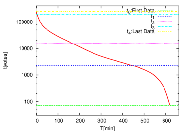
Figure 1: Relation between average time to start $T$ and average number of votes $t$.

Figure 1 shows the relation between $T$ and $t$. We see a rapid growth of the average number of votes $t$ as we approach the start of the race ($T\to 0$). Almost half of the votes are thrown in the last ten minutes. We choose five timings from the voting process and denote them as $t_{j},j\in\{0,1,2,3,4\}$. $t_{0}$ corresponds to the first voting data $k=1$ in each race. $t_{0}\simeq 70.4$ and $T(t_{0})\simeq 620.6$[min]. At $t_{1}\simeq 2342.9$, $T(t_{1})\simeq 440.2$[min]. At $t_{2}\simeq 15482.0$, $T(t_{2})\simeq 167.6$[min] and at $t_{3}\simeq 195201.3$, $T(t_{3})\simeq 2.5$[min]. $t_{4}$ corresponds to the last voting data $k=K_{r}$ in each race. $t_{4}\simeq 249708.8$ and $T(t_{4})\simeq-1.1$[min]. All data are summarized after the start of race. The reason why we choose $t_{i},i\in\{1,2,3\}$ will become clear in section 4.

In order to see the betting process pictorially, we arrange the $N$ horses in the order of the size of $x^{r}_{i}(t)$. We denote the arranged win bet fraction as $x_{\alpha}(t),\alpha\in\{1,2,\cdots,N\}$.

$$x_{1}(t)\geq x_{2}(t)\geq x_{3}(t)\geq\cdots\geq x_{N}(t)$$ (7)

$I_{\alpha}(t)$ tells us whether horse $\alpha$ wins ($I_{\alpha}=1$) or loses ($I_{\alpha}=0$). In general, the probability that the horse with large $x_{\alpha}(t)$ wins is big and vice versa. We arrange the horses in the increasing in order of $\alpha$ from left to right. On the left-hand side of the sequence, more strong horses exist. On the right-hand side, there are more weak horses. If the win bet fraction does not contain any information about the strength of the horses, $I_{\alpha}(t)$ is one and zero randomly. Conversely, if the information is perfectly correct, the first $N_{1}$ horses’ $I_{\alpha}(t)$ are 1 and the remaining $N_{0}$ horses’ $I_{\alpha}(t)$ are 0.

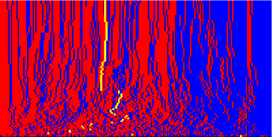
Figure 2: Pictorial presentation of the betting process. We choose 100 winning (red) and 100 losing (blue) horses randomly and follow their ranking as the betting proceeds. One losing horse is tagged by yellow dots.

Figure 2 shows the time change of the ranking process of the horses. We choose 100 horses for each category $I_{\alpha}=\{1,0\}$ and follow their ranking as the betting proceeds. We use $\Delta v=2000$ as the time step. During one hundred steps, the average number of votes $t$ changes from $t_{0}$ for $v=0$ (bottom) to about 178116 for $v=200000$ (top). $v=0$ corresponds to the first announcement $r=1$ and $t=t_{0}$. At $t_{0}$, the horses are arranged in the sequence at random. The win bet fractions $x_{\alpha}(t_{0})$ do not contain much information about the strength of the horses. As the betting progresses, the phase separation between the two categories of the horses does occur. Winning (losing) horses move to the left (right) in general. In the end, to the left (right) are more winning (losing) horses. In the betting process, betters have succeeded in choosing the winning horses to some extent. We also note that there remain winning horses in the right. This means that we can find winning horses with very small win bet fractions.

3 Emergence of scale invariance

In order to see the existence of a winning horse with a very small win bet ration or very low rank, we calculate the cumulative functions of the winning horses and that of the losing horses counted from the lowest rank (right). More precisely, we study the following quantities.

$$x_{\mu}(s)=\frac{1}{N_{\mu}}\sum_{\alpha=N(1-s)}^{N}\delta_{I_{\alpha},\mu}\hskip 5.69046pt,\hskip 5.69046pt\mu\in\{0,1\}$$ (8)

The above are normalized so that $x_{\mu}(s)$ is zero at $s=0$ and 1 at $s=1$. The curve $(x_{0}(s),x_{1}(s))$ is known as a receiver operating characteristic (ROC) curve. We are interested in the limit $s\to 0$. In particular, we study the scale invariant relation $x_{1}\propto x_{0}^{\alpha}$. If such a power law relation holds, we can find winning horses with any small win bet fraction.

(a)

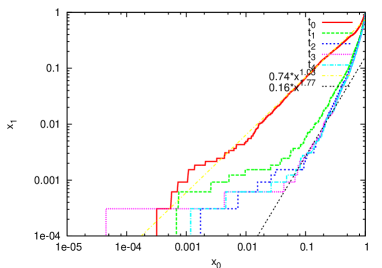
(b)

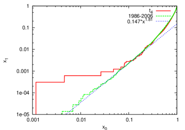
Figure 3: (a) Double-logarithmic plot of the ROC curve $(x_{0},x_{1})$. We plot four ROC curves for $t=t_{i},i\in\{0,1,2,3,4\}$. The fitted lines with $x_{1}=a\cdot x_{0}^{\alpha}$ for $t_{0}$ and $t_{3}$ are also plotted. (b) Double-logarithmic plot of the ROC curve $(x_{0},x_{1})$ for the data of all 1986-2006 JRA races. We also show the fitted line with $x_{1}=a\cdot x_{0}^{\alpha}$.

Figure 3a shows the double logarithmic plot of the ROC curves $(x_{0}(s),x_{1}(s))$. We show five curves for $t=t_{i},i\in\{0,1,2,3,4\}$. At $t=t_{0}$, there are 70 votes in the pool on average. The plot is almost a diagonal line from $(0,0)$ to $(1,1)$, which means that the winning and losing horses are mixed well in the sequence. The curve is fitted with the power relation $x_{1}=a\cdot x_{0}^{\alpha}$ with $\alpha=1.03$. As the betting progresses, the curve becomes more downward convex shape and the slope increases. At $t=t_{3},t_{4}$, the degree of the phase separation between the two types of horses reaches its maximum. On the other hand, we also see that there exist winning horses in the very low rank region. Each step upwards of the curve implies the existence of a winning horse and the upward movement starts for a very small $x_{0}$. In addition, we also see a straight line region in the curve in $0.03\leq x_{0}\leq 0.3$. We have fitted the curve as in the previous $(t_{0})$ case and we get $\alpha=1.77$. This means that the scale invariant relation between $x_{1}$ and $x_{0}$ also holds after many rounds of betting.

In order to see scale invariance more clearly, we show the same plot for the data of all JRA races from 1986 to 2006 in Figure 3b [6]. There are 71549 races and $N_{1}=71650$ and $N_{0}=829716$. The plot becomes straight in $0.003\leq x_{0}\leq 0.3$ with $\alpha=1.81$.

4 Emergence of efficiency

The win bet fraction aggregates the wisdom of the betters in the racetrack betting market. In order to quantify the accuracy, we use two measures. The first one is the accuracy ratio (AR). AR measures how an event occurs in the order of a rank. Here, we consider the event that a horse wins in the race. Horses are arranged in the increasing order of the size of the win bet fraction $x_{\alpha},\alpha\in\{1,2,\cdots N\}$. There are $N_{1}$ winning horses and $N_{0}=N-N_{1}$ losing horses. As we have explained before, if the prediction of the betters is good, the winning horses are concentrated in the higher ranks. If the prediction is perfect, the first $N_{1}$ horses are the winning ones and $I_{\alpha}$ is one for them. In order to define the accuracy of the prediction or to measure the completeness of the rank, we introduce a Lorenz curve $(x,\mbox{L}(x))$ for $0\leq x,\mbox{L}(x)\leq 1$ as

$$\mbox{L}(x)\equiv\frac{1}{N_{1}}\sum_{\alpha=1}^{N\cdot x}\delta_{I_{\alpha},1}.$$ (9)

(a)

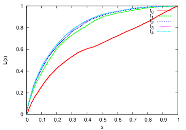
(b)

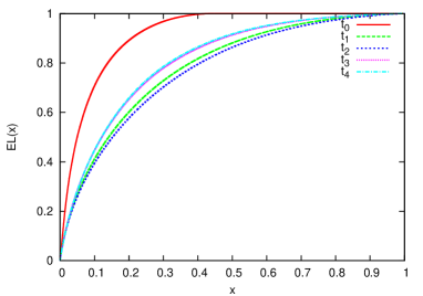
Figure 4: Plot of $(x,$L$(x))$ (a) and $(x,$EL$(x))$ (b) for $t=t_{i},i\in\{0,1,2,3,4\}$.

Figure 4a depicts the Lorenz curves for $t=t_{j},j\in{0,1,2,3,4}$. At $t=t_{0}$, after about seventy rounds, the horses are arranged at random on the sequence $\alpha\in\{1,2,\cdots,N\}$. The Lorenz curve runs almost along a diagonal line. As the betting proceeds, the winning horses ($I_{\alpha}=1$) move to the higher ranks and the degree of the upward convex nature of the curve increases. The preciseness of the prediction increases monotonically. At $t=t_{2}$, the increase almost stops and the accuracy of the predictions reaches a maximum.

In order to quantify the accuracy of the predictions of the racetrack betters, we use accuracy ratio, AR [12]. AR is defined as

$$\mbox{AR}\equiv(\int_{0}^{1}\mbox{L}(x)dx-\frac{1}{2})/\frac{1}{2}(1-\frac{N_{1}}{N}).$$ (10)

AR measures how different is the ranking from the complete case. The denominator in the definition is the normalization factor that ensures that AR is one for the completely ordered case. If the ranking is perfect, $\int_{0}^{1}L(x)dx-\frac{1}{2}=\frac{1}{2}(1-\frac{N_{1}}{N})$ and AR is 1.

We also introduce an expected Lorenz curve $(x,$EL$(x))$, which is defined as

$$\mbox{EL}(x)\equiv\frac{1}{R}\sum_{\alpha=1}^{N\cdot x}x_{\alpha}$$ (11)

[9]. In order to quantify how the bets are concentrated or scattered among horse, we introduce expected AR and call it EAR. EAR is defined as

$$\mbox{EAR}\equiv(\int_{0}^{1}\mbox{EL}(x)dx-\frac{1}{2})/\frac{1}{2}(1-\frac{R}{N}).$$ (12)

If we assume that the horses are divided into two groups, A and B. The horses’ win bet fraction in group A ($x_{\alpha},\alpha\in A$) is large and those of other horses in group B ($x_{\beta},\beta\in B$) is small, the votes are concentrated on the horses in group A. EAR is large. If the votes are scattered among all horses, EAR is small. In particular, if $x_{\alpha}=\frac{R}{N}$ for all $\alpha\in N$, EAR is zero. If $x_{\alpha}=1,\alpha\in A$ and $x_{\beta}=0,\beta\in B$, EAR is one.

Figure 4b depicts EL$(x)$ for $t=t_{j},j\in{0,1,2,3,4}$. At $t=t_{0}$, EL$(x)$ rapidly increases to one, which implies that votes are concentrated on small number of horses. However, AR is small at $t_{0}$ and the horses are not the winning horses. After $t_{0}$, the votes are scattered among many horses and the degree of the upward convex nature of the curve decreases up to $t_{2}$. After the decline, it begins to increases. At $t_{4}$, the degree of the concentration of votes reaches a maximum. $t_{2}$ is the boundary line. Before $t_{2}$, votes are more and more distributed among many horses. After $t_{2}$, the votes tend to be concentrated on popular horses.

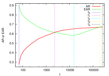
Figure 5: Plot of AR and EAR as the functions of $t$. The plot starts at $t_{0}$ and the two curves intersects at $t_{1}$ and $t_{3}$. At $t_{2}$, the discrepancy reaches its maximum after $t_{1}$.

By comparing the behaviour of L$(x)$ and EL$(x)$, we are able to study the efficiency of the market. If the probability that the horse $\alpha$ wins is $x_{\alpha}$, the two Lorenz curves L$(x)$ and EL$(x)$ do coincide with each other in the limit $N\to\infty$. Hence the equality $\mbox{AR}=\mbox{EAR}$ is a necessary condition of the efficiency of the market. However, it is not a sufficient condition. Even if the equality holds, there is a possibility that the two curves depart from each other. We also note that if the strength of the horse at rank $x$ is overvalued, the inequality $\mbox{L}^{\prime}(x)<\mbox{EL}^{\prime}(x)$ holds. On the contrary if the strength is undervalued, the inequality $\mbox{L}^{\prime}(x)>\mbox{EL}^{\prime}(x)$ holds. Here $\mbox{L}^{\prime}(x)=\frac{d\mbox{L}(x)}{dx}$ and $\mbox{EL}^{\prime}(x)=\frac{d\mbox{EL}(x)}{dx}$.

Figure 5 shows AR and EAR as the functions of $t$. As the betting progresses, AR increases monotonically and it almost reaches its maximum at $t=t_{2}$. Afterwards, the increase in AR is very slow and the following bets do not increase the accuracy of the prediction as to which horse wins the race. More interesting behaviour can be found in the time change of EAR. At $t=t_{0}$, EAR is very large and is nearly 0.9. Almost all votes are concentrated on small number of horses. However, AR at $t=t_{0}$ is small and the horses with large bet fractions are not so strong. The true strong horses are scattered all over the rank of the win bet fraction. Afterwords, EAR decreases rapidly and at $t=t_{1}$, AR and EAR coincide. The necessary condition of the market efficiency is satisfied at $t=t_{1}$. Up to $t=t_{2}$, EAR decreases and almost reaches its minimum. The bets are scattered among many horses and this implies the rich variety of the betters’ predictions as to which horse wins the race. This also means that the strong horses are undervalued and the weak horses are overvalued, that is the ‘favorite-longshot bias’ state, which can be seen more clearly below. The discrepancy between AR and EAR is the largest at $t=t_{2}$ after $t=t_{1}$. After that, the discrepancy decreases monotonically as EAR increases faster than AR. The bets begin to be concentrated on more popular horses. At $t=t_{3}$, AR and EAR coincide again. The necessary condition of the market efficiency is satisfied again. After $t_{3}$, the degree of the concentration increases further, the discrepancy between AR and EAR is small even at $t_{4}$.

(a)

(b)

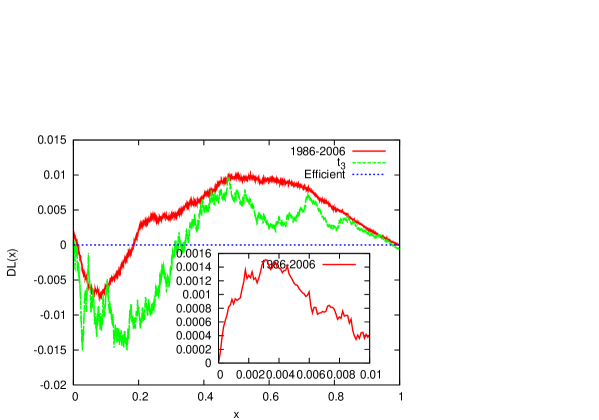
Figure 6: (a) Plot of DL$(x)\equiv\mbox{L}(x)-\mbox{EL}(x)$ for $t=t_{i},i\in\{0,1,2,3,4\}$. (b) Plot of DL$(x)$ for $t_{3}$ and all the data of JRA races $(1986-2006)$. Inset figure show the plot for all the data case for $0\leq x\leq 1\%$.

Figure 6a shows the discrepancies between $\mbox{L}(x)$ and $\mbox{EL}(x)$ at $t=t_{i},i\in\{0,1,2,3,4\}$. On the y-axis, we show $\mbox{DL}(x)\equiv\mbox{L}(x)-\mbox{EL}(x)$. As we have explained before, the sign of $\mbox{DL}^{\prime}(x)=\frac{d\mbox{DL}(x)}{dx}$ tells us whether the horse at rank $x$ is overestimated or underestimated. If $\mbox{DL}^{\prime}(x)$ is zero, the strength of the horse is properly estimated by the betters and the racetrack betting market is efficient. On the other hand, if $\mbox{DL}^{\prime}(x)$ is positive (negative), the strength is underestimated (oversetimated).

At $t=t_{1}$, DL$(x)$ is close to the x-axis and we see that for small $x\leq 20\%$, $\mbox{DL}(x)<0$. This means that the market is almost efficient, but top 10% popular horses are overestimated and next 10% horses are underestimated. Bets are more accumulated on the top 10% horses and their win bet fractions are larger than their true winning probabilities. On the other hand, there are less bets on next 10% horses as compared to their true winning probabilities. Remaining 80% horses’ strength are properly estimated, because DL$(x)$ is close to the x-axis. At $t=t_{2}$, $\mbox{DL}(x)$ is positive for all $0\leq x\leq 1$. From the figure, we see that the popular 30% horses are underestimated as compared to their winning probabilities. Remaining 70% unpopular horses are overestimated. The bets are distributed among many horses, including many weak horses and an inefficient state is realized. Following this, the graph of $\mbox{DL}(x)$ approaches the x-axis at $t=t_{3}$. The coincidence between the two Lorenz curves is better than at $t=t_{1}$. For small $x$ (popular horses), $\mbox{DL}(x)<0$ and the strong horses are overestimated. For large $x$ (unpopular horses), DL$(x)$ is almost on the x-axis. From the small discrepancy, we see that the top 20% horses are overestimated. And next 30% horses are underestimated. However, the slope of DL$(x)$ in the two regions is small and the market is almost efficient. This efficient state remains to be true even at $t_{3}$.

Figure 6b shows DL$(x)$ for the data of all JRA races (1986-2006). Contrary to the ‘favourite-longshot bias’, we see some complex behaviour. Top 0.4% horses are underestimated and next 10% horses are overestimated and so on. However, the degree of the inefficiency is very small.

5 Voting model and scale invariance

We consider a voting model for $N$ horses [6]. Betters vote for them one by one, and the result of each voting is announced promptly. The time variable $t\in\{0,1,2\cdots,T\}$ counts the number of the votes. The horses are classified into two categories $\mu\in\{0,1\}$, and we call them binary horses. There are $N_{\mu}$ horses in each category and $N_{0}+N_{1}=N$.

We denote the number of votes of the $i$th horse $\mu\in\{0,1\}$ at time $t$ as $\{X^{\mu}_{i,t}\}_{i\in\{1,\cdots,N_{\mu}\}}$. At $t=0$, $X_{i,t}^{\mu}$ takes the initial value $X_{i,0}^{\mu}=s_{\mu}>0$. If the $i$th candidate $\mu$ gets a vote at $t$, $X_{i,t}^{\mu}$ increases by one unit.

$$X_{i,t+1}^{\mu}=X_{i,t}^{\mu}+1.$$

A better casts a vote for the $N$ candidates at a rate proportional to $X_{i,t}^{\mu}$. The probability $P_{i,t}^{\mu}$ that the $i$th candidate $\mu$ gets a vote at $t$ is

$$P_{i,t}^{\mu} = \frac{X^{\mu}_{i,t}}{Z_{t}},$$ (13)

$$Z_{t} = \sum_{\mu=0}^{1}\sum_{i=1}^{N_{\mu}}X^{\mu}_{i,t}=N_{1}s_{1}+N_{0}s_{0}+t.$$ (14)

The problem of determining the probability of the $i$th candidate $\mu$ getting $n$ votes up to $T$ is equivalent to the famous Pólya’s urn problem [10, 11]. The probability that the $i$th candidate $\mu$ gets $n$ votes up to $T$ is given by the beta binomial distribution

$$\mbox{Prob}(X_{i,T}^{\mu}-s_{\mu}=n)={}_{T}C_{n}\cdot\frac{(s_{\mu})_{n}(Z_{0}-s_{\mu})_{T-n}}{(Z_{0})_{T}}.$$ (15)

$(a)_{n}$ is defined as $(a)_{n}=\frac{\Gamma(a+n)}{\Gamma(a)}$.

After infinite counts of voting, i.e. $T\to\infty$, the share of votes $x_{i}^{\mu}\equiv\lim_{T\to\infty}\frac{X_{i,T}^{\mu}-s_{\mu}}{T}$ becomes the beta distributed random variable beta$(s_{\mu},Z_{0}-s_{\mu})$ on $[0,1]$.

$$p(x) \equiv \lim_{T\to\infty}\mbox{Prob}(X_{i,T}^{\mu}-s_{\mu}=Tx)\cdot T$$ (16)

$$= \frac{x^{s_{\mu}-1}(1-x)^{Z_{0}-s_{\mu}-1}}{B(s_{\mu},Z_{0}-s_{\mu})}.$$

Next, we focus on the thermodynamic limit $N_{0},N_{1}\to\infty$ and $Z_{0}=N_{0}s_{0}+N_{1}s_{1}\to\infty$. The expectation value of $x_{i}^{\mu}$ is $<x_{i}^{\mu}>=p_{\mu}=\frac{s_{\mu}}{Z_{0}}$. We introduce a variable $u_{i}^{\mu}\equiv(Z_{0}-s_{\mu}-1)x_{i}^{\mu}$. The distribution function $p_{s_{\mu}}(u)$ in the thermodynamic limit is given as

$$p_{s_{\mu}}(u)\equiv\lim_{Z_{0}\to\infty}p(x_{i}^{\mu}=\frac{u}{Z_{0}-s_{\mu}-1})=\frac{1}{\Gamma(s_{\mu})}e^{-u}u^{s_{\mu}-1}.$$ (17)

The share of votes, $u$, of a candidate $\mu$ follows a gamma distribution function with $s_{\mu}$.

After many counts of voting, $T\to\infty$, the two types of horses are distributed in the space of $u$ according to the gamma distribution in the thermodynamic limit $Z_{0}\to\infty$. If $s_{1}>s_{0}$, a candidate belonging to category $\mu=1$ has a higher probability of getting many votes than a candidate belonging to category $\mu=0$. Even the latter can obtain many votes. It is also possible that the former may get few votes. Thus, there is a mixing of the binary candidates.

The cumulative functions $x_{\mu}(w)$ is given as

$$x_{\mu}(w)=\int_{0}^{w}p_{s_{\mu}}(u)du.$$ (18)

Using the incomplete gamma function of the first kind $\gamma(s,w)\equiv\int_{0}^{w}e^{-u}\cdot u^{s-1}du$, it is given as

$$x_{\mu}(w)=\frac{1}{\Gamma(s_{\mu})}\cdot\gamma(s_{\mu},w).$$ (19)

Near the end point, $w\to 0$, in other words, in the small $u$ region, the incomplete gamma function $\gamma(s_{\mu},t)$ behaves as

$$\gamma(s_{\mu},w)\sim w^{s_{\mu}}.$$ (20)

As $x_{s_{\mu}}(w)\propto w^{s_{\mu}}$, the following relation holds:

$$x_{1}\sim x_{0}^{\alpha}\hskip 11.38092pt\mbox{with}\hskip 11.38092pt\alpha=\frac{s_{1}}{s_{0}}.$$ (21)

We see that a scale invariant behaviour appears in the mixing.

Furthermore, in the limit $(s_{1},s_{0})\to(0,0)$ with fixed $\alpha=s_{1}/s_{0}$, next relation holds [6].

$$x_{1}=x_{0}^{\alpha}$$ (22)

The scale-invariant relation holds over the entire range $0\leq x_{0},x_{1}\leq 1$. This feature is remarkable from the viewpoint of statistical physics. Usually, the power-law relation holds only in the tail.

We discuss the limit in the derivation of the exact scale invariance. In the derivation of the gamma distribution, we take the thermodynamic limit $Z_{0}=N_{1}s_{1}+N_{0}s_{0}\to\infty$. With the gamma distribution, $x_{1}=x_{0}^{\alpha}$ holds in the limit $\{s_{\mu}\}\to 0$. For (22) to hold, these two limits, $Z_{0}\to\infty$ and $\{s_{\mu}\}\to 0$, should go together. $\{s_{\mu}\}$ approaches zero more slowly than $\{N_{\mu}\}$ approaches infinity. We call the limit $Z_{0}\to\infty$ and $\{s_{\mu}\}\to 0$ with fixed $\alpha=s_{1}/s_{0}$ as the double scaling limit. If we take the limit $\{s_{\mu}\}\to 0$ without the limit $Z_{0}\to\infty$, the firstly chosen candidate gets all the remaining votes and there is no mixing of the binary candidates. The double scaling limit is crucial to the emergence of the exact scale invariance.

6 Exact scale invariant gradation pattern

The voting problem reduces to a random ball removing problem with the relative probability $s_{\mu}$ in the double scaling limit [6]. Figure 11 shows the gradation pattern made by the algorithm of the random ball removing problem. We prepare $N_{1}$ red balls and $N_{0}$ blue balls. From them, we take one ball at a time and do not return it. The probability that a red (blue) ball is chosen is proportional to $s_{1}(s_{0})$. We repeat the procedure up to when there remains no ball. We get a sequence of $N=N_{1}+N_{0}$ balls. In the limit $N_{1},N_{0}\to\infty$, the exact scale invariance between $x_{1}$ and $x_{0}$ holds. In the figure, we change the ratio $\alpha=\frac{s_{1}}{s_{0}}$ from 1 (bottom) to 100 (top). Near the bottom, two types of balls are mixed. Near the top, phase separation occurs.

Figure 7: Exact scale invariant gradation pattern with varying $\alpha$ from $\alpha=1$ (bottom) to $\alpha=100$ (top).

7 Summary

In this paper, we study the time series of win bet fraction of the 2008 JRA races. We see that the betting process induces scale invariance between the cumulative functions of the winning horses and that of the losing horses. We also see the emergence of the market’s efficiency after many rounds of betting. However, the convergence to the efficient state is not monotonic. The dynamics of the distribution of the votes among the horses is complex. At first, the votes accumulate to small number of horses and then they are distributed among many horses, including weak horses. At this time, the strong horses are underestimated. Afterwards, votes begin to be concentrated on more popular horses, but the ranking of the winning horses does not change so much. AR does not change much and only EAR increases, and $\mbox{AR}=\mbox{EAR}$ finally holds.

With regard to the scale invariance, we explain the mechanism based on a simple voting model. The model shows exact scale invariance in the double scaling limit. In addition, the voting model in the limit is equivalent to a random ball removing problem. Using the equivalence, we show how to make an exact gradation pattern of mixed binary objects.

8 Acknowledgment

This research was partially supported by the Ministry of Education, Science, Sports and Culture, Grant-in-Aid for Challenging Exploratory Research, 21654054, 2009.

References

- [1] D.B.Hausch, V.SY.Lo and T.Ziemba, Efficiency of Racetrack Betting Markets 2008 Edition, World Scientific, Singapole.
- [2] R.M.Griffith, Amer.J.Psychol 62290(1949).
- [3] W.T.Ziemba and D.B.Hausch, Betting at the Racetrack ,Dr Z Investment Inc, San Luis Obispo, CA(1987).
- [4] K.Park and E.Dommany, Europhys.Lett. 53,419(2001).
- [5] T.Ichinomiya, Physica A368,207(2006).
- [6] S.Mori and M.Hisakado, Exact Scale Invariance in Mixing of Binary Candidates in Voting Model, preprint arXiv:0806.0185.
- [7] M.Hisakado and S.Mori, Phase Transition and Information Cascade in a Voting Model, preprint arXiv:0907.4818.
- [8] More precisely, we calculate before removing the cancelled horses from data. Up to the cancellation, these do not sum up to one. After cancellation, the odds and the win bet fraction become zero. These sum up to one.
- [9] If cancellation occurs in the betting process, the sum of is not before cancellation. In this case, it is necessary to divide by
- [10] G.Pólya, Ann.Inst.Henri Poincaré 1,117(1931).
- [11] M.Hisakado, K.Kitsukawa and S.Mori, J.Phys. A39,15365(2006).
- [12] B.Enleman, E.Hayden and D.Tasche, Testing Rating Accuracy, www.risk.net (2003).