Abstract

The Cartan model of ${\rm SO}(3)/{\rm SO}(2)$ matrices is applied to reduce of rotational degrees of freedom on coadjoint orbits of ${\rm u}^{\ast}(3)$ Poisson algebra. The seven–dimensional Poisson algebra ${\rm u}_{{\rm SO}}(3)$ obtained by ${\rm SO}(3)$ reduction of ${\rm u}^{\ast}(3)$ algebra is found and canonical parametrization of ${\rm u}^{\ast}(3)$ orbits $[p_{1},p_{2},p_{3}]{\vphantom{|}}_{\ast}$ is studied.

The structure of bands formed by so–called families of ${\mathsf{S}}$ and ${\mathsf{P}}$ ellipsoids obtained by searching extremes of many–body ${\rm SO}(3)$ invariant Hamiltonians is investigated.

The reduced four–dimensional system of equations of motion describing the simple schematic Hamiltonian based on the volume conservation is presented. A new set of canonical coordinates regarding the separation of motion for independent modes is found with the help of the Jacobi approach. Bohr Somerfield’s quantization of new momentum space is studied.

¹ Henryk Niewodniczański Institute of Nuclear Physics PAN, Department of Theoretical Physics, ul. Radzikowskiego 152, 31–342, Kraków, Poland

I Introduction

The aim of this paper is to discuss the simplest analytically solvable model describing the separation of collective degrees of freedom of many–particle dynamics into the pure rotational modes and the intrinsic one represented by ${\rm SO}(3)$ scalar functions.

The main role of the approach based on discussion of coadjoint orbits $[p_{1},p_{2},p_{3}]{\vphantom{|}}_{\ast}$ of ${\rm u}(3)$ algebra is to receive a preliminary description of the structure of equilibrium figures occurring in a more advanced and bristling with technical difficulties model based on coadjoint orbits $\langle p_{1},p_{2},p_{3}\rangle$ of ${\rm Sp}(6,R)$ group[1] and apply earlier studies[2, 3, 4, 5] employing the ${\rm Sp}(6,R)\times{\rm SO}(N-1)$ group for construction of a curvilinear system of coordinates on N–body phase space. The presented simplified model provides valuable results for explanation of some general features of the nuclear collective spectra of the ${\rm Sp}(6,R)$ model if the solutions describe almost spherical symmetric systems. The latter are selected forcing the conditions: $p_{1}-p_{2}\ll p_{3},p_{2}-p_{3}\ll p_{3}$.

The structure of Hamiltonian extremes on $[p_{1},p_{2},p_{3}]{\vphantom{|}}_{\ast}$ orbits is explained by considering two families of bands.

The first family of bands contains the equilibrium figures called ${\mathsf{S}}$ ellipsoids, while the second one contains ${\mathsf{P}}$ ellipsoids. Here ${\mathsf{S}}$ and ${\mathsf{P}}$ ellipsoids generalize the concept of ${\mathsf{S}}$ and ${\mathsf{P}}$ ellipsoids introduced by Riemann for classification of equilibrium figures of the Dirichlet, Dedekind, Riemann model[6].

In the paper we present the construction of a system of canonical coordinates on coadjoint orbits of ${\rm u}(3)$ regarding the reduction of dynamics of the ${\rm SO}(3)$ invariant system.

The first section employs elements of Cartan ${\rm SO}(3)/{\rm SO}(2)$ transformations in order to get

• ${\rm SO}(2)$ reduction of many particle phase space,

• Poisson bracket $\{.,.\}{\vphantom{|}}_{\ast}$ on ${\rm SO}(2)$ reduced space,

• reduction of ${\rm u}{{}^{\ast}}(3)$ to ${\rm u}_{\rm SO}(3)$.

In section III, four dimensional phase spaces $M^{\epsilon}_{\vec{p}}$ are applied to construct the canonical parametrization of $[p_{1},p_{2},p_{3}]{\vphantom{|}}_{\ast}$ orbits. In section IV, families of ${\mathsf{P}}$ and ${\mathsf{S}}$ ellipsoids are discussed. In section V, using a simple class of ${\rm SO}(3)$–scalar ${\rm u}{{}^{\ast}}(3)$ Hamiltonians and applying the Jacobi approach we obtain a new canonical parametrization $[p_{1},p_{2},p_{3}]{\vphantom{|}}_{\ast}$. In the last section, the quantum spectrum of the pair of new canonical momenta is searched with the help of Bohr Somerfield’s rules of quantization. Formulas determining the rules associated with point $(b)$ are found in Appendix.

II ${\rm SO}(3)$ reduced functions on orbits of $u{{}^{\ast}}(3)$ algebra

In the application of group transformation $({\mathsf{{\mathsf{G}}}},{\mathsf{M}})$ to Hamiltonian dynamics, elements of Lie algebra $U_{t}\!=\!\dot{g}_{t}\cdot{g_{t}}{{}^{-1}}\in\mbox{\eufm g}$ are obtained studying the mapping $t\to m_{t}=g_{t}\boldsymbol{\cdot}m_{0}$ under the assumption $g_{1}\cdot(g_{2}\boldsymbol{\cdot}m)\!=\!(g_{1}\cdot g_{2})\boldsymbol{\cdot}m$ and considering the following formula:

$$\dot{m}_{t}\!=\!\dot{g}_{t}\boldsymbol{\cdot}m_{0}=({\mathsf{U}}_{t}\cdot g_{t})\boldsymbol{\cdot}m_{0}\!=\!{\mathsf{U}}_{t}\boldsymbol{\cdot}m_{t}.$$ (1)

where $\dot{x}\!\equiv\!dx/dt$. In particular, in the case ${\mathsf{G}}\!=\!{\rm U}(3)$, $g_{t}$ are complex three dimensional matrices $g_{t}\cdot{g_{t}}{{}^{\dagger}}\!=\!\boldsymbol{1}$ for which Lie algebra is spanned by elements: $\mbox{\eufm g}\!=\!u(3)\!=\!\{{\mathsf{A}}=\Sigma_{\alpha\beta}\,{\mathsf{E}}_{ab}\,A_{\alpha\beta},\,A_{ab}\!=\!-A_{ba}{{}^{\ast}}\}$ where ${\mathsf{E}}_{ab}$ denote 3-dimensional matrices the elements of which read: $({\mathsf{E}}_{ab})_{cd}\!=\!\delta_{ac}\,\delta_{bd}$.

Within application to the particle dynamics, ${\rm U}(3)$ group follows from the study of group chain reduction ${\rm U}(3)\subset{\rm Sp}(6,R)\subset{\rm Sp}(6\,N,R)$ where ${\rm Sp}(6\,N,R)$ is the group of linear canonical transformations of $N$–particle space, while ${\rm Sp}(6,R)$ span the subspace of the collective one. Let $m\equiv\binom{\boldsymbol{a}^{1}}{\boldsymbol{a}^{2}},\,\boldsymbol{a}^{u}=(\vec{a}^{u}_{1},\ldots\vec{a}^{u}_{N}),\,u\!=\!1,2$ be a parametrization of points in $6\times N$ dimensional phase space. The application of ${\rm U}(3)$ group to the particle dynamics bases on the following formulas:

• $a^{u}_{an}\!=\!(2\,\kappa_{an}\,\hbar\,)^{-1/2}\,[p_{an}+(-1)^{u}\,i\,\kappa_{an}\,r_{an}]\!=\!(a^{3-u}_{an}){{}^{\ast}},\;a=x,y,z,\,n=1,\ldots,N$,

• $\Omega(p,r)=\Sigma_{in}\,p_{in}\wedge r_{in}\Leftrightarrow\{a^{u}_{an},a^{v}_{am}\}{\vphantom{|}}=-i\,(-1)^{u-1}\,\delta_{u\,3-v}\,\delta_{ab}\,\delta_{nm}$,

• $A_{ab}(m)=(a^{2}\cdot{{}^{\rm t\,}}a^{1})_{ab}-(\kappa^{-1}\,P_{a}+i\,\kappa\,X_{a})\,(\kappa^{-1}\,P_{b}-i\,\kappa\,X_{b})$,

• ${\mathsf{A}}(m)=\Sigma_{ab}\,A_{ab}(m)\,{\mathsf{E}}_{ab}\!=\!{\mathsf{A}}^{\dagger}(m)$,

• $A_{ab}(m)={\rm trace}\,{\mathsf{A}}(m)\cdot{\mathsf{E}}_{ba}$,

• ${\mathsf{A}}_{t}={\mathsf{A}}(m_{t})$, $m_{t}=\bigl{(}\begin{smallmatrix}{g_{t}}{{}^{\ast}}&\boldsymbol{0}\\ \boldsymbol{0}&g_{t}\end{smallmatrix}\bigr{)}\cdot m_{0}$ then ${\mathsf{A}}_{t}=g_{t}\cdot{\mathsf{A}}_{0}\cdot g^{-1}_{t}={\rm Ad}_{g_{t}}({\mathsf{A}}_{0})$ and $i\,{\mathsf{A}}(m)\in{\rm u}(3)$,

• $\dot{{\mathsf{A}}}_{t}=[{\mathsf{U}}_{t},{\mathsf{A}}_{t}]$, $\dot{x}_{t}\equiv\tfrac{d~{}}{dt}x_{t}$,

• ${\mathsf{A}}(m)=\sum_{\mu}Z^{\mu}(m)\;{{}^{\rm t\mspace{1.0mu}}}{\mathsf{Z}}_{\mu}=\sum_{\mu\nu}G_{\mu\nu}[{\mathsf{Z}}]\,Z_{\mu}(m)\,{{}^{\rm t\mspace{1.0mu}}}{\mathsf{Z}}_{\mu}$,

• $\{Z_{\mu},Z_{\nu}\}_{m}=-i\,{\rm trace}\,{\mathsf{A}}(m)\cdot{{}^{\rm t}}\,[{\mathsf{Z}}_{\mu},{\mathsf{Z}}_{\nu}]$,

where $\kappa_{an}=\omega_{a}\,{\mathsf{m}}_{n}$, $\kappa_{n}=\omega\,{\mathsf{m}}_{n}$, $\omega_{x}\!=\!\omega_{y}\!=\!\omega_{z}\!=\!\omega$, $({\mathsf{m}}_{1},\ldots,{\mathsf{m}}_{N})$ are the particle masses, $Z_{\mu}(m)$ and ${\mathsf{Z}}_{\mu}$ are components of vectors $\vec{Z}(m)\!=\!(Z_{1}(m),\ldots,Z_{9}(m))$ and the vector of matrices $[{\mathsf{Z}}]\!=\![{\mathsf{Z}}_{1},\ldots,{\mathsf{Z}}_{9}]$, respectively. We chose them using two pairs of bases: $(\vec{Z}_{\mathbb{C}}(m),[{\mathsf{Z}}_{\mathbb{C}}])$ or $(\vec{Z}_{\mathbb{R}}(m),[{\mathsf{Z}}_{\mathbb{R}}])$ where $\vec{Z}_{\mathbb{R}}(m)\!=\!\lambda(\vec{Z}_{\mathbb{C}}(m))$ and $[{\mathsf{Z}}_{\mathbb{R}}]\!=\!\kappa([{\mathsf{Z}}_{\mathbb{C}}])$. Here,

• $\kappa$:   ${\mathsf{L}}_{a}=-i\,\Sigma_{bc}\,\epsilon_{abc}\,{\mathsf{E}}_{bc}$, ${\mathsf{Q}}_{ab}=\tfrac{1}{2}\,({\mathsf{E}}_{ab}+{\mathsf{E}}_{ba})$,

• $\lambda$:   ${\mathsf{L}}_{a}(m)=-i\,\Sigma_{bc}\,\epsilon_{abc}\,A_{bc}(m),\,{\mathsf{Q}}_{ab}(m)=\tfrac{1}{2}\,(A_{ab}(m)+A_{ba}(m))$,

• $\kappa{}^{(-1)}$:   ${\mathsf{E}}_{ab}={\mathsf{Q}}_{ab}+\tfrac{i}{2}\,\Sigma_{k}\,\epsilon_{abc}\,{\mathsf{L}}_{c}$,  $\lambda{}^{(-1)}$:   $A_{ab}(m)={\mathsf{Q}}_{ab}(m)+\tfrac{i}{2}\,\Sigma_{c}\,\epsilon_{abc}\,{\mathsf{L}}_{c}(m)$,

hence

• ${\mathsf{L}}_{a}(m)\!=\!\Sigma_{bc}\,\epsilon_{abc}\,[\Sigma_{n}x_{an}\,p_{bn}-X_{a}\,P_{b}]=2\,{\mathsf{L}}^{a}(m)\in\mathbb{R}$,

• ${\mathsf{Q}}_{ab}(m)=\tfrac{1}{2}\,[\Sigma_{n}(\kappa_{n}\,x_{an}\,x_{bn}+{\kappa_{n}}{{}^{-1}}\,p_{an}\,p_{bn})-\kappa\,{X_{a}}{{}^{2}}-\kappa^{-1}\,{P_{a}}{{}^{2}}=(2-\delta_{ab})^{-1}\,{\mathsf{Q}}^{ab}(m)\in\mathbb{R}$,

• ${\mathsf{A}}(m)=\sum_{a}{\mathsf{L}}^{a}(m)\,{\mathsf{L}}_{a}+\sum_{a<b}{\mathsf{Q}}^{ab}(m)\,{\mathsf{Q}}_{ab}$,

where $\kappa=N^{-1}\,\Sigma^{N}_{n=1}\kappa_{n}$. The second term in ${\mathsf{L}}_{ab}(m),{\mathsf{Q}}_{ab}(m)$ and $A_{ab}(m)$ subtract the contribution resulting from the center of mass coordinates–momenta: $X_{a}={\mathsf{M}}^{-1}\,\Sigma_{n}\,{\mathsf{m}}_{n}\,x_{an},\,P_{\alpha}=\Sigma_{n}\,p_{an}$. The following formulas hold

• $G[{\mathsf{Z}}]\cdot g[{\mathsf{Z}}]\!=\!\boldsymbol{1}$, $g_{\mu\nu}[{\mathsf{Z}}]={\rm trace}\,{\mathsf{Z}}_{\mu}\cdot{\mathsf{Z}}_{\nu}$,

• $[{\mathsf{Z}}_{\mathbb{C}}]=[{\mathsf{E}}_{xx},{\mathsf{E}}_{xy},\ldots,{\mathsf{E}}_{zz}]$, $g_{({\mathsf{E}}_{ab},{\mathsf{E}}_{cd})}[{\mathsf{Z}}_{\mathbb{C}}]=\delta_{ad}\,\delta_{bc}$,

• $[{\mathsf{Z}}_{\mathbb{R}}]\!=\![{\mathsf{L}}_{x},{\mathsf{L}}_{y},{\mathsf{L}}_{z},{\mathsf{Q}}_{xx},{\mathsf{Q}}_{yy},{\mathsf{Q}}_{zz},{\mathsf{Q}}_{xy},{\mathsf{Q}}_{yz},{\mathsf{Q}}_{zx}]$, $g_{\mu\nu}[{\mathsf{Z}}_{\mathbb{R}}]\!=\!({\rm diag}\,(2,2,2,1,1,1,\tfrac{1}{2},\tfrac{1}{2},\tfrac{1}{2}))_{\mu\nu}$,

The most essential points are $(d)$ and $(e)$ considered under the assumptions ${\mathsf{U}}_{t}\!=\!{\mathsf{U}}(A_{t})$. Indeed, if we put

$$({\mathsf{U}}_{t})_{ab}=-(\partial_{A_{ba}}\,H)({\mathsf{A}}_{t}),$$ (2)

then, the system at point $(e)$ is closed and it is equivalent to the Hamiltonian equation of motion $\dot{A}_{\mu}=\{A_{\mu},H(A)\}$. The proof of points $(g,h)$ is elementary if the pair of bases $[Z_{\mathbb{C}}(m)]$ and $[{\mathsf{Z}}_{\mathbb{C}}]$ is applied. Since the coefficients of transformations $\kappa$ and $\lambda$ coincide, points $(g,h)$ have to be valid for the pair ($[Z_{\mathbb{R}}]$,$[{\mathsf{Z}}_{\mathbb{R}}]$), too.

Further reduction of the set of equations of motion at the point $(f)$ and assumption (2) are obtained assuming the symmetry of Hamiltonian $H\!=\!H(A)$.

In order to discuss the reduction generated by ${\rm SO}(3)$ invariance: $\{{\mathsf{L}}_{a},H\},\,a\!=\!x,y,z$ let us introduce a mapping $\vec{r}\equiv(r_{x},r_{y},r_{z})=(x,y,z)\to[(x,y,z)]\in{\mathsf{K}}\subset{\rm SO}(3)$:

$$[(x,y,z)]=\begin{pmatrix}1-a^{2}&-ab&\bar{x}\\ -\epsilon\,a\,b&1-b^{2}&\bar{y}\\ -\bar{x}&-\bar{y}&\bar{z}\end{pmatrix},\qquad\quad\begin{matrix}(a,b)=(|\vec{r}|\,d)^{-1/2}\,(x,y),\\ (\bar{x},\bar{y})=|\vec{r}|^{-1}\,(x,y),\\ d=|\vec{r}|+z,\end{matrix}$$ (3)

and a pair of nonlinear coordinate transformations $$\Lambda_{\pm 1}$$:

$$\mathbb{C}^{3\times N}\setminus\mathbb{C}_{\pm}\ni a\to b\in S_{\pm}\!=\!\{b\in\mathbb{C}_{3\times N},\,\vec{{\mathsf{L}}}({\mathsf{A}}(\boldsymbol{b},\boldsymbol{b}{{}^{\ast}}))\!=\!(0,0,\pm|\vec{{\mathsf{L}}}|)\},$$ (4)

$$(b^{u}_{1m},b^{u}_{2m},b^{u}_{3m})=(a^{u}_{xm},a^{u}_{ym},a^{u}_{zm})\cdot[\pm\vec{{\mathsf{L}}}({\mathsf{A}}(\boldsymbol{a},\boldsymbol{a}{{}^{\ast}}))],$$ (5)

$$b^{1}\equiv b,\qquad b^{2}\equiv b{{}^{\ast}},$$ (6)

$$\mathbb{C}_{\pm}\!=\!\{a\in\mathbb{C}^{3\times N},\,\vec{{\mathsf{L}}}({\mathsf{A}}(a,a{{}^{\ast}}))\neq(0,0,\mp|\vec{{\mathsf{L}}}|)\}.$$ (7)

${\mathsf{K}}$ is called the Cartan model of factor space ${\rm SO}(3)/{\rm SO}_{\vec{e}_{3}}(2)$:

• $[\alpha\,\vec{x}\,]\!=\![{\rm sign}\,(\alpha)\,\vec{x}]$,

• $[\vec{x}\,]\cdot\vec{e}_{3}=|\vec{x}|^{-1}\,\vec{x}$,

• $[\vec{x}\,]\cdot\vec{x}{{}_{\ast}}\!=\!|\vec{x}|\,\vec{e}_{3}$, $\vec{x}{{}_{\ast}}={{}^{\rm t\mspace{1.0mu}}}(-x_{1},-x_{2},x_{3})$,

• $[\vec{x}{{}_{\ast}}]=[\vec{x}]^{-1}$,

• $[[\vec{x}\,]\cdot\vec{a}\,]\!=\![\vec{x}\,]\cdot[\vec{a}\,]$,

• $[\vec{x}\,]\cdot(\vec{x}\times\vec{e}_{3})=\vec{x}\times\vec{e}_{3}$,

• $[\vec{x}\,]=[\vec{e}_{3}\times\vec{x}]\cdot R_{3}(\alpha)\cdot[(\vec{e}_{3}\times\vec{x}){{}_{\ast}}]\in{\rm SO}_{\vec{e}_{3}\times\vec{x}}(2)$, $(\cos\alpha,\sin\alpha)\!=\!|\vec{x}|^{-1}\,(\sqrt{{x_{1}}{{}^{2}}+{x_{2}}{{}^{2}}},x_{3})$,

where ${\rm SO}_{\vec{u}}(2)=\{g\in{\rm SO}(3),\,g\cdot\vec{x}=\vec{x}\}$, $R_{3}(\alpha)=\cos\alpha\,({\mathsf{E}}_{11}+{\mathsf{E}}_{22})+\sin\,\alpha\,({\mathsf{E}}_{21}-{\mathsf{E}}_{12})+{\mathsf{E}}_{33}$ and $|\vec{x}|=({{}^{\rm t\mspace{1.0mu}}}\vec{x}\cdot\vec{x})^{1/2}$.

Replacing $m\!=\!m(a^{1},a^{2})\to m(b^{1},b^{2})=\bar{m}$ and ${\rm SO}(3)$ tensor $({\mathsf{L}},{\mathsf{Q}})\to(L,Q)$ we get

$$B_{ij}(\bar{m})=\sum_{n}\,b^{2}_{in}\,b^{1}_{jn}=Q_{ij}(\bar{m})+\tfrac{i}{2}\,\Sigma_{k}\,\epsilon_{ijk}\,L_{k}(\bar{m}),\qquad L_{i}(\bar{m})\equiv 0,\,i=1,2,$$ (8)

$$B_{ij}\circ\bar{m}(m)=\sum_{ab}\,[ai]\,[bj]\,A_{ab},\qquad[ai]=[\epsilon\,\vec{{\mathsf{L}}}({\mathsf{A}}(\boldsymbol{a},\boldsymbol{a}{{}^{\ast}}))]_{m(a)i}.$$ (9)

where $m(x)\!=\!1,m(y)\!=\!2,m(z)\!=\!3$.

Definition 1

. $u^{\ast}_{{\rm SO}}(3)$ is algebra $\{.,.\}{\vphantom{|}}_{\ast}$ spanned by seven elements

$$(L_{3},\,Q_{1},Q_{2},Q_{3},q_{1},q_{2},q_{3}),\qquad Q_{i}\equiv Q_{ii},\;\;q_{1}\equiv Q_{23}\,{\rm cycl}\,1,2,3.$$

Let $B_{ij}\!=\!B_{ij}{{}^{\ast}}$ and $B_{3k}=B_{k3},\,k\!=\!1,2$ be the functions introduced according to eq.$(\ref{Bij})$. The Poisson rules result from the following relations:

$$\{B_{i_{1}i_{2}},B_{j_{1}j_{2}}\}{\vphantom{|}}_{\ast\,B}=-i\,(\delta_{i_{2}j_{1}}\,B_{i_{1}j_{2}}-\delta_{\i_{1}j_{2}}\,B_{j_{1}i_{2}})$$

$$+{L_{3}}{{}^{-1}}\,\sum_{kl}(\gamma^{kl}_{i_{1}j_{1}}\,B_{ki_{2}}\,B_{lj_{2}}+\gamma^{kl}_{i_{2}j_{1}}\,B_{i_{1}k}\,B_{lj_{2}}+\gamma^{kl}_{i_{1}j_{2}}\,B_{ki_{2}}\,B_{j_{1}l}+\gamma^{kl}_{i_{2}j_{2}}\,B_{i_{1}k}\,B_{j_{1}l}),$$ (10)

where $${\rm sign}\,L_{3}\!=\!\pm 1 (\ref{toP1*},\ref{toP*})$$ depends on the choice of a sign in the map and

$$\gamma^{kl}_{ij}=\delta_{k3}\,(\delta_{j3}\,\epsilon_{il3}-\delta_{l3}\,\epsilon_{ij3})-\delta_{i3}\,(\delta_{l3}\,\epsilon_{jk3}+\delta_{j3}\,\epsilon_{kl3}).$$ (11)

Formulas (10) are elementary derived by the substitution $B_{ij}=\Sigma_{k}\,b^{2}_{in}\,b^{u}_{jn}$ (see eq.(8, 10)) and assuming the following relations:

$$\{b^{u}_{in},b^{v}_{jm}\}{\vphantom{|}}_{b}=-i\,(-1)^{u-1}\,\delta_{u\,3-v}\,\delta_{ij}\,\delta_{nm}+\Gamma_{ij}(\vec{b}^{u}_{n},\vec{b}^{v}_{m},L_{3}),$$ (12)

$$\Gamma_{ij}(\vec{a},\vec{b},z)=z^{-1}\,\sum_{kl}\gamma^{kl}_{ij}\,a_{k}\,b_{l},$$ (13)

Proof of formulas (11,12,13) is studied in Appendix. Algebra $u^{\ast}_{{\rm SO}}(3)$ decomposes $u^{\ast}_{{\rm SO}}(3)={\rm su}^{\ast}_{{\rm SO}}(3)\times C_{1}$ where $C_{1}={\rm trace}\,{\mathsf{B}}\!=\!\Sigma_{i\leq 3}\,Q_{i}\!=\!Q_{1}+Q_{2}+Q_{3}$ is the centrum while ${\rm su}^{\ast}_{{\rm SO}}(3)\!=\!\{L,\bar{Q}_{1},\bar{Q}_{2},q_{1},q_{2},q_{3}\}$ where $\bar{Q}_{1}=2^{-1/2}\,(Q_{1}-Q_{2}),\bar{Q}_{2}=6^{-1/2}\,(2\,Q_{3}-Q_{1}-Q_{2})$. For the matrix ${\mathsf{B}}=\Sigma_{ij}\,B_{ij}\,{\mathsf{E}}_{ij}$ we get

$${\mathsf{B}}=\begin{pmatrix}Q_{1}&q_{3}+\tfrac{i}{2}L_{3}&q_{2}\\ q_{3}-\tfrac{i}{2}L_{3}&Q_{2}&q_{1}\\ q_{2}&q_{1}&Q_{3}\end{pmatrix},$$ (14)

where $q_{3}\equiv Q_{12},\,{\rm cycl}\,1,2,3$. From formulas (8,10) we get

$$\{Q_{k},L_{3}\}{\vphantom{|}}_{\ast}=0,\qquad\{q_{3},L_{3}\}{\vphantom{|}}_{\ast}=Q_{1}-Q_{2},\qquad\{q_{i},L_{3}\}{\vphantom{|}}_{\ast}=(-1)^{i-1}\,q_{3-i},$$ (15a)

$$\{Q_{i},Q_{j}\}{\vphantom{|}}_{\ast}=-4\,(\Sigma_{k}\epsilon_{ijk})\,L^{-1}\,q_{1}\,q_{2},$$ (15b)

$$\{q_{1},q_{2}\}{\vphantom{|}}_{\ast}={L_{3}}{{}^{-1}}\,[(Q_{1}-Q_{3})\,(Q_{2}-Q_{3})-{q_{3}}^{2}-{\mathsf{G}}\,{L_{3}}{{}^{2}}/4],$$ (15c)

$$\{q_{i},q_{3}\}{\vphantom{|}}_{\ast}={L_{3}}^{-1}\,(-1)^{i-1}\,[q_{3-i}\,q_{3}+q_{i}\,(Q_{3}-Q_{3-i})],$$ (15d)

$$\{Q_{i},q_{j}\}{\vphantom{|}}_{\ast}=\frac{2}{L_{3}}\,\begin{pmatrix}q_{2}\,(Q_{2}-Q_{3})&q_{2}\,q_{3}&\tfrac{{\mathsf{G}}\,{L_{3}}^{2}}{4}-{q_{2}}^{2}\\ q_{3}\,q_{1}&q_{1}\,(Q_{3}-Q_{1})&{q_{1}}{{}^{2}}-\tfrac{{\mathsf{G}}\,{L_{3}}^{2}}{4}\\ q_{3}\,q_{1}+(Q_{3}-Q_{2})\,q_{2}&-q_{2}\,q_{3}-(Q_{3}-Q_{1})\,q_{1}&-{q_{1}}{{}^{2}}-{q_{2}}{{}^{2}}\end{pmatrix}_{ij}.$$ (15e)

where the Poisson rules for coalgebra $u^{\ast}_{\rm SO}(3)$ we find putting ${\mathsf{G}}\!=\!1$. If $L_{1}\equiv L_{2}\equiv 0$ then $\{L_{1},x\}{\vphantom{|}}_{\ast}=\{L_{2},x\}{\vphantom{|}}_{\ast}=0$ are fulfilled for all $x\in u^{\ast}_{\rm SO}(3)$ identically.

The case ${\mathsf{G}}\!=\!0$ is also physically interesting. Assuming $Q|_{{\mathsf{G}}\!=\!0}=\mbox{\rsfs Q}$ one finds $\{\mbox{\rsfs Q}_{ab},\mbox{\rsfs Q}_{cd}\}\!=\!0$ and $\{{\mathsf{L}}_{a},\mbox{\rsfs Q}_{bc}\}=\sum_{d}\,(\epsilon_{abd}\,\mbox{\rsfs Q}_{dc}+\epsilon_{acd}\,\mbox{\rsfs Q}_{bd})$; hence, $({\mathsf{L}},\mbox{\rsfs Q})$ is the semidirect Poisson algebra obtained considering the mass quadrupole–monopole tensor: $\mbox{\rsfs Q}=\Sigma_{k}{\mathsf{m}}_{k}\,\vec{x}_{k}\otimes\vec{x}_{k}-{\mathsf{M}}\,\vec{X}\otimes\vec{X}$ where the center of mass reference frame is applied.

III Canonical coordinates on $[p_{1},p_{2},p_{3}]_{\ast}$ orbits.

Coadjoint orbits of $u{{}^{\ast}}(3)$ coalgebra are found studying a surface ${\rm U}(3)\ni g\to{\mathsf{A}}(g\boldsymbol{\cdot}m_{0})={\rm Ad}_{g}(m_{0})$. These orbits denoted as $[p_{1},p_{2},p_{3}]$ are labeled by components of the weight vector $\vec{p}=(p_{1},p_{2},p_{3})$ accordingly with the following Casimir relations:

$$C_{k}({\mathsf{A}})\!=\!S_{k}(\vec{p}),\qquad C_{k}({\mathsf{A}})\!=\!{\rm trace}\,{\mathsf{A}}_{k},\qquad{\mathsf{A}}_{1}\!=\!{\mathsf{A}},\quad{\mathsf{A}}_{k+1}={\mathsf{A}}_{k}\cdot{\mathsf{A}}_{1},$$ (16)

where $S_{k}(\vec{p})\equiv S_{k}$. Here $S_{k}$, as well, a few other ones

$$S_{k}\equiv\Sigma_{i\leq 3}\,{p_{i}}{{}^{k}},\qquad$$ (17)

$$S_{k1}=(1+\delta_{k1})^{-1}\,\Sigma_{l}(p_{l+1}+p_{l+2})\,{p_{l}}{{}^{k}},$$ (18)

$$S_{111}=p_{1}\,p_{2}\,p_{3},\quad S^{B}_{111}=(p_{1}-p_{2})\,(p_{2}-p_{3})\,(p_{1}-p_{3}),$$ (19)

$$S^{A}_{111}=(p_{1}+p_{2}-2\,p_{3})\,(p_{2}+p_{3}-2\,p_{1})\,(p_{1}+p_{3}-2\,p_{2}).$$ (20)

are frequently used functions of $\vec{p}$. The A peculiar class of orbits will be discussed here. They are obtained using the assumptions: $p_{1}\!>\!p_{2}\!>\!p_{3}$.

The ${\rm SO}(3)$ reduction of $u{{}^{\ast}}(3)$: $u{{}^{\ast}}(3)\to u^{\ast}_{\rm SO}(3)$ constraint $[p_{1},p_{2},p_{3}]$, ${\rm dim}[p_{1},p_{2},p_{3}]=6$ to four dimensional orbits $[p_{1},p_{2},p_{3}]{\vphantom{|}}_{\ast\hat{\epsilon}}$. Casimir functions $C_{k}$ for $k\!=\!1,2,3$ are independent.

Choosing $(q_{1},q_{2},Q_{3},L_{3})$ as a set of independent coordinates, let us rewrite three Casimir relations (see, eq.(16,17)) in the following form:

$$Q_{+}\!=\!\tfrac{1}{2}\,(S_{1}-Q),\qquad\begin{pmatrix}{q_{1}}^{2}-{q_{2}}^{2}&2\,q_{1}\,q_{2}\\ -2\,q_{1}\,q_{2}&{q_{1}}^{2}-{q_{2}}^{2}\end{pmatrix}\binom{q_{3}}{Q_{-}}=\binom{V_{L}(Q,R)}{U(Q,R)}.$$ (21)

where

$$U(Q,R)\!=\!G_{\vec{p}}(Q)+\tfrac{3}{2}\,(Q-\langle p\rangle)\,R^{2},$$ (22)

$$V_{L}(Q,R)=\epsilon\,[-\hat{w}_{\vec{p}}(L,Q,R)]^{1/2}.$$ (23)

and $\epsilon\!=\!\pm 1$. The following formulas have been applied

$$Q\equiv Q_{3},\qquad Q_{\pm}\equiv\tfrac{1}{2}\,(Q_{1}\pm Q_{2}),\qquad L\equiv L_{3},\qquad R^{2}\equiv{q_{1}}^{2}+{q_{2}}^{2},$$ (24)

$$\langle p\rangle=\tfrac{1}{3}\,S_{1},\qquad G_{\vec{p}}(x)=\prod_{i}(x-p_{i}),$$ (25)

$$\hat{w}_{\vec{p}}(a,b,c)=\tfrac{1}{4}\,b^{4}\,a^{2}+H_{\vec{p}}(b,c),$$ (26)

$$H_{\vec{p}}(b,c)=\prod_{i<j}h_{ij}(b,c),\qquad h_{ij}(b,c)=(b-p_{i})\,(b-p_{j})+c^{2},$$ (27)

New coordinates $(p,\gamma)$ are determined introducing a pair of relations

$${R_{L,Q,p}}{{}^{2}}=-\frac{G_{\vec{p}}(Q)}{Q-p},\qquad\cos^{2}\gamma_{L,Q,p}=\frac{L^{2}}{4}\,\frac{Q-p}{G_{\vec{p}}(p)}.$$ (28)

They define mapping $\Lambda_{L}\!:(p,\gamma)\to(Q,R)=(Q_{\vec{p},L}(p,\gamma),R_{\vec{p},L}(p,\gamma))$ where

$$R_{\vec{p},L}(p,\gamma)=(2\,L^{2}\,|\cos\gamma|)^{-1}\,\sqrt{-F_{\vec{p},L}(p,\gamma)},$$ (29)

$$Q_{\vec{p},L}(p,\gamma)\!=\!p+4\,L^{-2}\,G_{\vec{p}}(p)\,\cos^{2}\gamma,$$ (30)

$$F_{\vec{p},L}(p,\gamma)=\prod_{i\leq j}\,\hat{h}_{ij}(L,p,\gamma),\qquad\hat{h}_{ij}(a,b,\gamma)=a^{2}+4\,(p_{i}-b)\,(p_{j}-b)\,\cos^{2}\gamma.$$ (31)

Simple calculations lead to the following two identities

$$H_{\vec{p}}\circ\Lambda(p,\gamma)=-(2\,L\,\cos\gamma)^{-6}\,{F_{\vec{p}}}{{}^{2}}(L,p,\gamma)=-\frac{L^{2}\,{R_{\vec{p},L}}{{}^{4}}(p,\gamma)}{4\,\cos^{2}\gamma},$$ (32)

$$V_{\vec{p},L}(p,\gamma)=V_{L}\circ\Lambda_{L}(p,\gamma)=\tfrac{1}{8}\,L^{-3}\,F_{\vec{p},L}(p,\gamma)\,\cos^{-3}(\gamma)\,\sin\,\gamma,$$ (33)

where the function $F_{\vec{p},L}(Q,R)$ (presented in eq.(31)): $(a)$ is negative valued on ${\mathsf{M}}^{\pm}_{\vec{p}}$ (see, eq.(29)) and $(b)$ is an even function of $\gamma$; so $V_{\vec{p},L}(p,\gamma)$ is

• an odd function of $\gamma$,

• ${\rm SO}(3)$ scalar function,

and,

• ${\rm sign}\,\sin\,\gamma\!=\!-{\rm sign}\,V_{L}=-\epsilon$.

Employing point $(c)$ we get the following form of the inverse transformation $(Q,R)\to(p,\gamma)\!=\!(p_{\vec{p}}(Q,R),\gamma_{L,Q,R})$:

$$p_{\vec{p}}(Q,R)=Q+R^{-2}\,G_{\vec{p}}(Q),$$ (34)

$$\binom{\cos\gamma_{L,Q,R}}{\sin\gamma_{L,Q,R}}=\frac{1}{\sqrt{-H_{\vec{p}}(Q,R)}}\times\binom{\frac{L\,R^{2}}{2}}{-V_{L}(Q,R)}.$$ (35)

where $\epsilon_{\gamma}\!=\!{\rm sign}\,\gamma$, and we assumed $\sqrt{\smash[b]{|x|}}\geq 0$. Let us define $\Gamma\!:{\mathsf{M}}^{\hat{\epsilon}}_{\vec{p}}\ni(L,p,\varphi,\gamma)=m\to\Gamma(m)=(q_{1},q_{2},q_{2},Q_{1},Q_{2},Q_{3},L_{3})\in[\vec{p}]{\vphantom{|}}_{\ast\hat{\epsilon}}$ where

$$L_{3}\!=\!L,\qquad Q_{1}\!=\!Q_{+}+Q_{-},\quad Q_{2}=Q_{+}-Q_{-},\qquad Q_{3}\!=\!Q_{\vec{p},L}(p,\gamma),$$ (36a)

$$Q_{+}=\tfrac{1}{2}\,[S_{1}-Q_{\vec{p},L}(p,\gamma)],$$ (36b)

$$q_{1}+i\,q_{2}=e^{-i\,\varphi}\,(2\,L^{2}\,\cos\gamma)^{-1}\,\sqrt{\smash[b]{-F_{\vec{p},L}(p,\gamma)}},$$ (36c)

$$Q_{-}+i\,q_{3}=e^{i\,2\,\varphi}\,[\tfrac{3}{2}\,(p-\langle p\rangle)-\tfrac{i}{2}\,L\,\tan\gamma+2\,L^{-2}\,G_{\vec{p}}(p)\,\cos^{2}\gamma],$$ (36d)

The sets ${\mathsf{M}}^{\hat{\epsilon}}_{\vec{p}}=\Gamma{}^{(-1)}([\vec{p}]{\vphantom{|}}_{\ast\hat{\epsilon}})$ are discussed below. Signatures $\hat{\epsilon}={\rm sign}\,L_{3}$ result from the choice of ${\rm SO}(3)$ matrices $[\hat{\epsilon}\,\vec{L}]$ determining the coordinates $b$ (see, eq.(5)).

Theorem 1

. $\Gamma({\mathsf{M}}^{\hat{\epsilon}}_{\vec{p}})=[\vec{p}]{\vphantom{|}}_{\ast{\hat{\epsilon}}}$ for ${\mathsf{M}}^{\hat{\epsilon}}_{\vec{p}}\!=\!\bigcup_{0<\,\hat{\epsilon}\,L}{\mathsf{M}}_{2,\vec{p},L}\setminus(\overline{{\mathsf{M}}_{3,\vec{p},L}}\cup\overline{{\mathsf{M}}_{1,\vec{p},L}})$ where

$${\mathsf{M}}_{i,\vec{p},L}=\{(L,p,\varphi,\gamma),\;\varphi\equiv\varphi\,{\rm Mod}(2\,\pi),\,0<\cos\gamma,\,p^{-}_{i,\vec{p}}\,(L\,\sec\gamma)<p<p^{+}_{i,\vec{p}}\,(L\,\sec\gamma)\},$$

$$p^{\pm}_{i,\vec{p}}(l)\!=\!\frac{1}{2}\,\left(p_{i+1}+p_{i+2}\pm\sqrt{(p_{i+1}-p_{i+2})^{2}-l^{2}}\right),\quad p_{k}\equiv p_{1+{\rm Mod}_{3}(k)},$$

The sets $\overline{{\mathsf{M}}^{\hat{\epsilon}}_{i,\vec{p}}}$ closes ${\mathsf{M}}^{\hat{\epsilon}}_{i,\vec{p}}$ where $\overline{{\mathsf{M}}^{\hat{\epsilon}}_{i,\vec{p}}}=\bigcup_{\hat{\epsilon}\,L>0}\overline{{\mathsf{M}}^{\hat{\epsilon}}_{i,L,\vec{p}}},\,\overline{{\mathsf{M}}^{\hat{\epsilon}}_{i,L,\vec{p}}}\!=\!\{(L,p,\varphi,\gamma),\,\varphi\equiv\varphi\,{\rm Mod}(2\,\pi),\,0<\cos\,\gamma,\;f_{i}(L,p,\gamma)\leq 0\}$ and $f_{1}(L,p,\gamma)=\hat{h}_{23}(L,p,\gamma),\,{\rm cycl}\,1,2,3$ $[$see eq.$(\ref{toF})]$.
      The pairs $(\varphi,L)$ and $(\gamma,p)$ are mutually commuting canonical coordinates such that

$$\Omega_{M^{\pm}_{\vec{p}}}(m)\!=\!dL\wedge d\varphi\mp dp\wedge d\gamma,$$ (37)

If $l\leq{\rm min}\,(p_{1}-p_{2},p_{2}-p_{3})$ then $p^{\pm}_{i,\vec{p}}(l)\in\mathbb{R}$ and $p^{-}_{2,\vec{p}}(l)\!\leq\!p^{-}_{1,\vec{p}}(l)<p^{+}_{1,\vec{p}}(l)\leq p^{-}_{3,\vec{p}}(l)<p^{+}_{3,\vec{p}}(l)\!\leq\!p^{+}_{2,\vec{p}}(l)$.

The reduction of range for $\gamma\!:\,\cos\,\gamma\!>\!0$ results from the identity: $\Gamma(L,p,\varphi+\pi,\gamma+\pi)=\Gamma(L,p,\varphi,\gamma)$.

Subspaces ${\mathsf{M}}^{\sigma}_{i,\vec{p},}$ obey the following rules:

• ${\mathsf{M}}^{\hat{\epsilon}}_{2,\vec{p},L}\neq\emptyset\Leftrightarrow\hat{\epsilon}\,L\leq p_{1}-p_{3}$,

• ${\mathsf{M}}^{\hat{\epsilon}}_{3,\vec{p},L}\neq\emptyset\Leftrightarrow\hat{\epsilon}\,L\leq p_{1}-p_{2}$,

• ${\mathsf{M}}^{\hat{\epsilon}}_{1,\vec{p},L}\neq\emptyset\Leftrightarrow\hat{\epsilon}\,L\leq p_{2}-p_{3}$,

• ${\mathsf{M}}^{\hat{\epsilon}}_{2,\vec{p},L}\cap{\mathsf{M}}_{i,\vec{p},L}\!=\!{\mathsf{M}}_{i,\vec{p},L}$

• ${\mathsf{M}}^{+}_{i,\vec{p},L}\cap{\mathsf{M}}^{-}_{j,\vec{p},L}=\emptyset$.

Proof of theorem 1. Applying to formulas $(\ref{su3crul})$ the rules of coordinate transformation obtained from mapping $(\varphi,R)\to(q_{1},q_{2})$ and choosing the coordinates $(q_{1},\ldots,q_{4})=(\varphi,L,Q,\\ R)$ one finds

$$\{\varphi,L\}{\vphantom{|}}_{\ast}=1,\qquad\{\varphi,Q\}{\vphantom{|}}_{\ast}=2\,L^{-1}\,R^{-2}\,G_{\vec{p}}(Q),$$

$$\{\varphi,R\}{\vphantom{|}}_{\ast}=(L\,R)^{-1}\,[3\,Q^{2}+R^{2}-2\,S_{1}\,Q+S_{11}+\tfrac{1}{4}\,(1-G)\,L^{2}],$$

$$\{L,Q\}{\vphantom{|}}_{\ast}=\{L,R\}{\vphantom{|}}_{\ast}=0,\qquad\{Q,R\}{\vphantom{|}}_{\ast}=2\,L^{-1}\,R^{-1}\,V_{L}(Q,R).$$

Let $\hat{\omega}^{-1}=\omega$ where $\hat{\omega}\!:\,\hat{\omega}_{ij}\!=\!\{q_{i},q_{j}\}$. Then $\Omega_{G}(\varphi,L,Q,R)=\sum_{i\leq j}\,\omega_{ij}\,dq_{i}\wedge dq_{j}$ is a symplectic two–form. The explicit calculation gives

$$\Omega_{\textsf{G}}(\varphi,L,Q,R)=dL\wedge(d\varphi+\omega_{LQ}\,dQ+\omega_{LR}\,dR)+\omega_{RQ}\,dR\wedge dQ,$$ (38)

$$\omega_{LR}=(V_{L}\,R)^{-1}\,G_{\vec{p}}(Q),$$ (39)

$$\omega_{RQ}=\tfrac{1}{2}\;{V_{L}}{{}^{-1}}(Q,R)\,L\,R,$$ (40)

$$\omega_{LQ,\textsf{G}}=(2\,V_{L})^{-1}(Q,R)\,[-3\,Q^{2}+2\,S_{1}\,Q-S_{11}-R^{2}+\tfrac{1}{4}\,(\textsf{G}-1)\,L^{2}].$$ (41)

With the help of relations

• $dp=(1+R^{-2}\,G^{\prime}_{\vec{p}}(Q))\,dQ-2\,R^{-3}\,G_{\vec{p}}\,dR$,

• $d\gamma=-\cot\,\gamma\,[L^{-1}\,dL-\tfrac{1}{2}\,\,{H_{\vec{p}}}{{}^{-1}}\,H{}^{(1,0)}_{\vec{p}}\,dQ+(2\,R^{-1}-\tfrac{1}{2}\,{H_{\vec{p}}}{{}^{-1}}\,H{}^{(0,1)})\,dR]$,

• $\cot\gamma=-\tfrac{1}{2}\,{V_{L}}{{}^{-1}}\,L\,R^{2}$,

• $dp\wedge d\gamma={V_{L}}^{-1}\,[\,R^{-1}\,G_{\vec{p}}\;dR\wedge dL+\tfrac{1}{2}\,R^{2}\,(1+R^{-2}\,G^{\prime})\,dL\wedge dQ+u\,dQ\wedge dR]$,

• $u\!=\!(4\,H_{\vec{p}}\,R)^{-1}\,L\,[2\,G\,H{}^{(1,0)}_{\vec{p}}-4\,H\,(R^{2}+(G_{\vec{p}})^{\prime})+R\,H{}^{(0,1)}_{\vec{p}}(R^{2}+(G_{\vec{p}})^{\prime})]\!=\!\tfrac{1}{2}\,L\,R,$

we find $dp\wedge d\gamma=\omega_{LR}\,dL\wedge dR+\omega_{LQ,1}\,dL\wedge dQ+\omega_{RQ}\,dR\wedge dL$ which proves the statement.

IV Ellipsoids

The ${\rm su}^{\ast}_{\rm SO}(3)$ Hamiltonians are ${\rm SO}(3)$ invariant if $0\!\equiv\!H_{,\varphi}\Rightarrow\bar{H}\!=\!H_{L}(p,\gamma)$. The function $V_{L}$ commutes with angular momentum: $\{V_{L},\,L\}{\vphantom{|}}_{\ast}\!=\!0$; hence, the most general form of the function $H_{L}(p,\gamma)$ is obtained using (in general independent) two functions $\bar{h}_{i,L}(Q,R)$

$$H_{L}(p,\gamma)=h_{1,L}(p,\gamma)+h_{2,L}(p,\gamma)\times V_{L}\circ\Gamma(p,\gamma),$$ (42)

$$h_{i,L}(p,\gamma)=\bar{h}_{i,L}\circ\Gamma_{L}(p,\gamma),$$ (43)

where the second term of $H_{L}(p,\gamma)$ represents $\gamma$ odd contribution. Since

$$R_{,L}(p,\gamma)\equiv(\partial_{L}R_{\vec{p},L})(p,\gamma)=L^{-1}\,{R_{\vec{p},L}}^{-1}(p,\gamma)\times(R^{2}+3\,Q^{2}-2\,S_{1}\,Q+S_{11}),$$ (44)

$(\partial_{L}\,h_{i,L})(Q,0)$ is finite only if $|\lim_{R\to 0}R^{-1}\,h{}^{((0,1))}_{i}(Q,R)|\!<\!\infty$.

Let

$$\Omega_{\vec{p},L}(p,\gamma)\!=\!H_{L,L}(p,\gamma),\qquad\Lambda_{\vec{p},L}(p,\gamma)=H_{L,p}(p,\gamma),$$ (45)

denote first derivatives of Hamiltonian $H_{L}(p,\gamma)$.

Definition 2

. Points $m=(L,p,\varphi,\gamma_{i,p})$ of sets $\partial{\mathsf{M}}_{i,\vec{p},L}$ are selected from the following conditions:

$$p\in[p^{-}_{i,\vec{p}}(L),p^{+}_{i,\vec{p}}(L)],\qquad L\in[0,p_{i>}-p_{i<}],\qquad\binom{p_{i<}}{p_{i>}}=\binom{{\rm min}(p_{i+1},p_{i+2})}{{\rm max}(p_{i+1},p_{i+2})},$$ (46)

$$\cos\gamma_{i,p}\!=\!\frac{L}{2\,\sqrt{p_{i>}-p}\,\sqrt{p-p_{i<}}},\qquad i=1,2,3,$$ (47)

We have:

• $Q\!=\!Q(m)=Q_{L}(p,\cos\gamma_{i,p})=p_{i}$.

• $R_{\vec{p},L}(p,\gamma_{i,p})\!=\!0$.

Definition 3

. The states $\partial{\mathsf{M}}_{i,\vec{p},L}$ are called ${\mathsf{S}}_{{\mathsf{i}}}$–ellipsoids. The condition $\Lambda_{\vec{p},L}(p,\gamma)\!=\!0$ selects the family of ${\mathsf{P}}$ ellipsoids.

Here and further physical states $m$ will be described using the map ${\mathsf{M}}^{+}_{\vec{p}},({\mathsf{M}}_{i,\vec{p}}\equiv{\mathsf{M}}^{+}_{i,\vec{p}})$: $L\!=\!L(m)>0$.

${\mathsf{S}}_{{\mathsf{i}}}$ ellipsoids: $L\!=\!p_{i>}-p_{i<}\!=\!L_{i,\rm max},\,i=1,2,3$ we call the maximal states. For maximal states

• $p^{-}_{i,\vec{p}}(L_{i,\rm max})\!=\!p^{+}_{i,\vec{p}}(L_{i,\rm max})=\tfrac{1}{2}\,(p_{i<}+p_{i>})$

• $\gamma\!=\!\gamma_{p}\!=\!0$,

• $q_{1}-q_{2}\!=\!Q_{-}\!=\!0\Rightarrow\Gamma(L_{i,\rm max},\tfrac{1}{2}\,(p_{i<}+p_{i>}),\varphi+\alpha,0)=\Gamma(L_{i,\rm max},\tfrac{1}{2}\,(p_{i<}+p_{i>}),\varphi,0)$.

i.e., they are axially–symmetric states (see point $(c)$).

The discussion of the family of ${\mathsf{P}}$ ellipsoids becomes much simpler in the cases when $H(L,p,\gamma)$ is an even function of coordinates $\gamma$: $H(L,p,\gamma)\!=\!H(L,p,-\gamma)$. Since

$$H_{,p}(L,p,0)=0,\qquad p\neq p_{i},\;i=1,2,3,$$ (48)

these extremes exist for $\gamma\!=\!0$. As a natural example let us discuss ${\mathsf{P}}$–ellipsoids for the following Hamiltonians:

$$H_{\omega,g}(L,Q)\!=\!E_{0}+\tfrac{1}{4}\,\omega(L)\,Q,$$ (49)

The physical role of this family is exhibited by the following formula:

$${\rm det}\,{\mathsf{Q}}=p_{1}\,p_{2}\,p_{3}+\tfrac{1}{4}\,Q\,L^{2}.$$ (50)

The simple subfamily is derived considering the functions

$$H_{\omega,r,s}({\mathsf{Q}})=\kappa^{-1}(s)\,\omega_{\langle r\rangle}\,{\langle\vec{p}\rangle_{g}}{{}^{1-3\,\kappa(s)}}\,{\rm det}^{\kappa(s)}\,{\mathsf{Q}},$$ (51)

$$\qquad\kappa(s)=\frac{6\,s}{s+2},\qquad\omega_{\langle r\rangle}=(p_{V}/{\langle\vec{p}\rangle_{g}}{})^{r-1}\times\omega,$$ (52)

where $\omega$ is the nuclear constant $\hbar\,\omega=\hbar\,\omega_{\mathsf{A}}\approx 40\,{\mathsf{A}}^{-1/3}\,{\rm MeV}$, ${\langle\vec{p}\rangle_{g}}{}\!=\!(p_{1}\,p_{2}\,p_{3})^{1/3}\approx p_{V}$ where $p_{V}\equiv\tfrac{1}{6}\,(3\,{\mathsf{A}}/2)^{4/3}\,\hbar$ is simple estimation of the Pauli selection rule for a neutron–proton system resulting from application of the triaxially deformed harmonic oscillator shell model. Assuming $\omega(L)\ll\omega_{V}$, then preserving the linear term and comparing the result with formula, eq.(49), we get

$$\omega(L)\approx{\langle\vec{p}\rangle_{g}}{{}^{-2}}\,\omega_{\langle r\rangle}\,L^{2},$$ (53)

as well

$$\Omega_{i,r}(0)=(\partial_{p_{i}}H_{\omega,s,r})(0)=\frac{(2-r)\,(2+s)}{2\,s}\times\frac{\omega_{\langle r\rangle}\,{\langle\vec{p}\rangle_{g}}{}}{p_{i}},$$ (54)

where ${\langle\vec{x}\rangle_{g}}{}\!=\!(x_{1}\,x_{2}\,x_{3})^{1/3}$. As in the physical model $\Omega_{i,r}(0)$ has to be positive, the physical range of parameters $(s,r)$ is limited by the conditions: $r\leq 2$ and $0\leq s$.

If $r\!=\!r_{\rm h.o.}$, where $r_{\rm h.o.}\!=\!4/(2+s)$, then $\Delta E_{\vec{p}}(0)\!=\!E_{\vec{p}+\delta\vec{p}}=\Sigma_{i}\,\Omega_{i,r}(0)\,\delta p_{i}+\ldots$ is power series of the excitation energy. One finds

$$\Omega_{\vec{p},L}(p,\gamma)=\frac{s\,p\,L\,H_{\omega,r,s}}{3\,(2+s)},\quad\Lambda_{\vec{p},L}(p,\gamma)=\frac{s\,[L^{2}-{\mbox{\rsfs L}_{\vec{p}}}{{}^{2}}(p)\,\cos^{2}\gamma]}{6\,(2+s)}\,H_{\omega,r,s},$$ (55)

$$\mbox{\rsfs L}_{\vec{p}}(p)=2\,\sqrt{-3\,p^{2}+2\,p\,S_{1}-S_{11}}.$$ (56)

The functions $\mbox{\rsfs L}_{\vec{p}}(p)$ fulfill the following rules:

• $\mbox{\rsfs L}_{\vec{p}}\,(p_{\pm}(L))\equiv L$,

• $p_{\sigma}(\mbox{\rsfs L}_{\vec{p}}(p))=p$ if $\sigma\,(S_{1}-3\,p)>0$,

• $p_{\sigma}(\mbox{\rsfs L}_{\vec{p}}(p))=\tfrac{1}{3}\,(2\,S_{1}-p)$ if $\sigma\,(S_{1}-3\,p)<0$,

where $\sigma\!=\!\pm 1$ and

$$p_{\pm}(L)=\tfrac{1}{3}\,\bigl{(}S_{1}\mp S_{L}),\qquad S_{L}=\tfrac{1}{2}\,\sqrt{-3\,L^{2}+4\,(S_{2}-S_{11})}.$$ (57)

The conditions $p=p_{\pm}(L,\vec{p})$ select the family of ${\mathsf{P}}_{+}$ and ${\mathsf{P}}_{-}$ ellipsoids, respectively.

The physical interpretation of the functions $p_{\pm}(L)$ is provided by the following theorem:

Theorem 2

. Tensor ${\mathsf{Q}}$ possesses degenerated eigenvalues $P_{1}\!=\!P_{2}\geq P_{3}$ if and only if $p=p_{+}(L)$ and $P_{1}>P_{2}\!=\!P_{3}$ if and only if $p=p_{-}(L)$.

In order to prove theorem 2, we have to check the validity of the following rules:

• formula (70),

• the relation $V_{\vec{p}}(L,Q,x)\!=\!-\tfrac{1}{4}\,L^{2}(Q_{L,\vec{p}}(x,0)-Q)$ (see also, eq.(67)), and,

• pair of identities: $(\partial_{x}Q_{L,\vec{p}})(x,0)|_{x=p_{\pm}(L)}=0$.

The explicit expressions for eigenvalues $P_{\alpha}$ found from equation (70) are studied in a number of relations (77–80). Let ${\mathsf{D}}_{\vec{p}}$ denote the set obtained from projection of ${\mathsf{M}}_{\vec{p}}$ onto the plane $(L,Q)$. Using formulas, eq.(80), we find

$${\mathsf{D}}_{\vec{p}}=\bigcup_{0\leq L\leq p_{1}-p_{3}}(L,[Q^{L}_{\rm min},Q^{L}_{\rm min}]),$$ (58)

$$Q^{L}_{\rm min}=\begin{cases}p_{3}&0\leq L\leq\lambda,\\ \bar{Q}_{-}(L)&\lambda\leq L\leq h(\lambda,\mu),\\ p_{2}&h(\lambda,\mu)\leq L\leq\lambda+\mu,\end{cases}\qquad Q^{L}_{\rm max}=\begin{cases}p_{1}&0\leq L\leq\mu,\\ \bar{Q}_{+}(L)&\mu\leq L\leq h(\mu,\lambda),\\ p_{2}&h(\mu,\lambda)\leq L\leq\lambda+\mu\end{cases}$$ (59)

$$\bar{Q}_{\sigma}(L)\!=\!Q_{L,\vec{p}}(p_{\sigma}(L),0),$$ (60)

$$h(x,y)=\sqrt{(x+y)^{2}-{\min}^{2}(x-y,0)}=\begin{cases}x+y&x\geq y,\\ 2\,\sqrt{x\,y}&{\rm else.}\end{cases}$$ (61)

where $\bar{Q}_{\sigma}(L)$ obey the following identity: $V_{\vec{p}}(L,\,\bar{Q}_{\sigma}(L),p_{\sigma}(L))\equiv 0$ for $V_{\vec{p}}(L,Q,p)$ given in eq.(67). Formulas, eqs.(57,60), separate on orbits $[\vec{p}]{\vphantom{|}}_{\ast}$ two bands ${\mathsf{P}}_{-}$ and ${\mathsf{P}}_{+}$:

$${\mathsf{P}}_{\pm}\!:\quad\gamma=0,\qquad p\!=\!p_{\pm}(L),\quad Q=\bar{Q}_{\sigma}(L).$$ (62)

Angular momentum range in the case of ${\mathsf{P}}_{-}$ band is equal to $L\in[\lambda,h(\lambda,\mu)]$, while for ${\mathsf{P}}_{+}$ band: $L\in[\mu,h(\mu,\lambda)]$ (see, eq.(59).

The function $S_{L}$ is real if $L^{2}\leq\bar{L}^{2}\!=\!\frac{4}{3}\,(S_{2}-S_{11})\!=\!{L_{\rm max}}^{2}+\tfrac{1}{3}\,(\lambda-\mu)^{2}$ where $L_{\rm max}\!=\!\lambda+\mu$ is maximal physical value of angular momentum. Hence, $S_{L}$ is positive valued function. One finds

$$\bar{E}_{i}={\rm det}\,{\mathsf{Q}}({\mathsf{S}}_{{\mathsf{i}}})=p_{i}\,(p_{i+1}\,p_{i+2}+\tfrac{1}{4}\,L^{2}),$$ (63)

$$\bar{E}_{\pm}={\rm det}\,{\mathsf{Q}}({\mathsf{P}}_{\pm})=S_{111}+\tfrac{1}{27}\,S^{A}_{111}+\tfrac{1}{4}\,\langle p\rangle\,L^{2}-\tfrac{1}{18}\,(p_{\pm}(L,\vec{p})-\langle p\rangle)^{3/2},$$ (64)

where by $\bar{E}_{3}<\bar{E}_{2}<\bar{E}_{1}$ we denoted values of the energy factor ${\rm det}\,{\mathsf{Q}}$ in the cases of ${\mathsf{S}}_{{\mathsf{i}}}$ ellipsoids, while $\bar{E}_{-}<\bar{E}_{+}$ determine the energy factor in the case of ${\mathsf{P}}_{-}$ and ${\mathsf{P}}_{+}$ ellipsoids, respectively.

It is interesting to compare the derived expression onto solutions for ${\mathsf{S}}_{{\mathsf{i}}}$ bands with the earlier study[5] of the model of ${\mathsf{S}}$–ellipsoids based on the orbits $\langle p_{1},p_{2},p_{3}\rangle$ of ${\rm sp}{{}^{\ast}}(6,R)$ Poisson algebra. For the many–particle system bounded by the ${\rm SO}(N)\times{\rm SO}(3)$ invariant potential: $U(\mbox{\rsfs Q})\!=\!(s+2)^{-1}\,H_{\omega,2,s}(m\,\omega_{\mathsf{A}}\,\mbox{\rsfs Q})$ the system of condition selecting ${\mathsf{S}}_{{\mathsf{i}}}$ ellipsoids reduces. In the limit $p_{i+1}-p_{i+2}\ll p_{i+1}+p_{i+2}$ the asymptotic formulas read

$${\rm det}\,(m\,\omega_{\mathsf{A}}\,\mbox{\rsfs Q})\approx{\rm det}\,{\mathsf{Q}}({\mathsf{S}}_{{\mathsf{i}}}),\qquad L\leq|p_{i+1}-p_{i+2}|,$$ (65)

where $\mbox{\rsfs Q}_{ab}=({\mathsf{A}}/{\mathsf{M}})\,\Sigma_{k=1}^{\mathsf{A}}\,\,m_{k}\,(x_{\alpha k}-X_{\alpha})\,(x_{\alpha k}-X_{\alpha})$ is the mass quadrupole–monopole tensor, $\vec{X}$ is the center of mass vector, while the total energy equal to $E_{\langle\vec{p}\rangle}(L,{\mathsf{S}}_{{\mathsf{i}}})\!=\!T+U(\mbox{\rsfs Q})\approx{3\,(s+2)}\,(2\,s)^{-1}\,\omega_{\langle r\!=\!2\rangle}\,{\langle\vec{p}\rangle_{g}}{{}^{1-\kappa(s)}}\,{\bar{E}_{i}}{{}^{\kappa(s)/3}}$ restates the formula onto the total energy obtained here. The same formulas (for $r\!=\!2$ and $s\!=\!2$) have been derived much earlier [7] by investigating a simplified form of a cranked harmonic oscillator model in which the ${\rm U}(3)$ tensor terms of [2,0,0] and [0,0,-2] type have been neglected in the procedure of diagonalization of the Routhian function: $H_{\vec{\omega},\Omega}=\sum_{a}\omega_{a}\,A_{aa}(m)-\Omega\,L_{z}(m)|_{\vec{\omega}=(\omega_{x},\omega_{y},\omega_{z})}$.

For $(L,p,\gamma)\in{\mathsf{M}}^{+}_{\vec{p}}$ one finds:

• ${\mathsf{P}}_{-}\cap{\mathsf{S}}_{{\mathsf{3}}}\!=\!(p_{1}-p_{2},p_{3},0)$,

• ${\mathsf{P}}_{+}\cap{\mathsf{S}}_{{\mathsf{3}}}\!=\!(p_{2}-p_{3},p_{1},0)$,

and if $\mu<\lambda$ then

• ${\mathsf{P}}_{-}\cap{\mathsf{S}}_{2}\!=\!(p_{1}-p_{3},p_{2},0)$ and ${\mathsf{P}}_{+}\cap{\mathsf{S}}_{2}\!=\!(2\,\sqrt{\lambda\,\mu},p_{2},0)$,

else,

• ${\mathsf{P}}_{+}\cap{\mathsf{S}}_{2}\!=\!(p_{1}-p_{3},p_{2},0)$ and ${\mathsf{P}}_{-}\cap{\mathsf{S}}_{2}\!=\!(2\,\sqrt{\lambda\,\mu},p_{2},0)$.

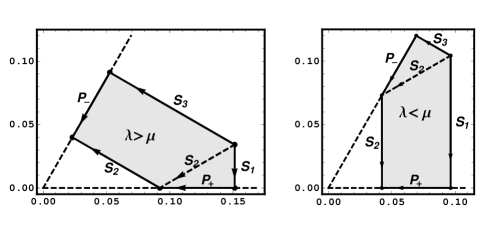
Figure 1: The projection of $(\lambda,\mu)$ states onto the $(\beta,\Gamma)$ plane

The structure of ${\mathsf{S}}$ and ${\mathsf{P}}$ bands on $[\vec{p}]{\vphantom{|}}_{\ast}$ depends on the sign of expression $\lambda-\mu$.

If $\mu<\lambda$, then the minima of $H\!=\!{\rm det}({\mathsf{Q}})$ form two bands:

• ${\mathsf{S}}_{3}$ for $0<L\leq\lambda$, and,

• ${\mathsf{P}}_{-}$ for $\lambda\leq L\leq\lambda+\mu$ ellipsoids,

while hamiltonian maxima decouple into three bands:

• ${\mathsf{S}}_{1}$ for $0\leq L\leq\mu$,

• ${\mathsf{P}}_{+}$ for $\mu\leq L\leq 2\,\sqrt{\mu\,\lambda}$, and,

• ${\mathsf{S}}_{2}$ for $2\,\sqrt{\mu\,\lambda}\leq L\leq\lambda+\mu$,

If $\lambda<\mu$ hamiltonian minima decouple into three bands:

• ${\mathsf{S}}_{3}$ for $0\leq L\leq\lambda$,

• ${\mathsf{P}}_{-}$ for $\lambda\leq L\leq 2\,\sqrt{\mu\,\lambda}$, and,

• ${\mathsf{S}}_{2}$ for $2\,\sqrt{\mu\,\lambda}\leq L\leq\lambda+\mu$,

while hamiltonian maxima form two bands:

• ${\mathsf{S}}_{1}$ for $0\leq L\leq\mu$, and,

• ${\mathsf{P}}_{+}$ for $\mu\leq L\leq\lambda+\mu$.

In both the cases ${\mathsf{S}}_{2}$ ellipsoids for $0\leq L\leq 2\,\sqrt{\smash[b]{\lambda\,\mu}}$ are vibrationally unstable states.

The graphic representation of two structures of equilibrium bands found for a family of orbits $(a)$ $\mu<\lambda$ and $(b)$ $\lambda<\mu$ are studied on Figure 1. the $(\lambda,\mu)$ states of ${\rm su}{{}^{\ast}}(3)$ orbit are projected on the $(\beta,\Gamma)$ plane: $(x,y)=(\beta\,\cos\Gamma,\beta\sin\Gamma)$. The parameters $(x,y)$ fix the eigenvalues $(P_{1},P_{2},P_{3})$ according to the rules presented in eqs.(77, 78).

The left graphic is obtained for the values $(\lambda,\mu,p_{3})=(50,15,100)$ while the right for $(15,50,100)$. ${\mathsf{S}}_{i}$ and ${\mathsf{P}}_{\pm}$ ellipsoids close the set of $(\lambda,\mu)$ states represented by the shadowed area. If $\mu\leq\lambda$, then parameter $\Gamma$ of the maximal state $L\!=\!\lambda+\mu$ is equal to $\Gamma\!=\!60\textdegree$ (prolate ellipsoid) else $\Gamma\!=\!0\textdegree$ (oblate ellipsoids). On both pictures, the angular momentum of ellipsoids increases accordingly with the direction of arrows.

V Wobbling motion for Hamiltonian $H=E_{0}+\tfrac{1}{4}\,\omega(L)\,Q$.

V.1 Canonical pair of coordinates conjugated to momenta $(L,Q)$

Coordinates $L,Q$ commute, so $L,Q\!=\!Q_{L}(p,\gamma)$ are constants of motion of Hamiltonians $H\!=\!H_{\omega,r,s=2}$; hence, $H\!=\!H(L,p,\gamma)\!=\!h_{0}+\tfrac{1}{4}\,\omega(L)\,Q$. Then $\dot{p}=-H{}^{(0,0,1)}(L,p,\gamma)=2\,L^{-2}\,G_{\vec{p}}(p)\,\omega(L)\,\cos\gamma\,\sin\,\gamma$ where according to the second relation in eq.(28) on the surface $Q\!=\!{\rm const},L\!=\!{\rm const}$: $\gamma=\epsilon_{\gamma}\,\gamma^{+}_{L,Q,p}$, $\epsilon_{\gamma}={\rm sign}\,\gamma$, $\gamma^{\pm}_{L,Q,p}=-i\,\ln Z^{\pm}_{\vec{p}}(L,Q,p)$ where

$$Z^{\pm}_{\vec{p}}(L,Q,p)={G_{\vec{p}}}{{}^{-1/2}}(p)\,\bigl{[}\tfrac{L}{2}\,\sqrt{\smash[b]{Q-p}}\pm i\,\sqrt{\smash[b]{-V_{\vec{p}}(L,Q,p)}}\bigr{]},$$ (66)

$$V_{\vec{p}}(L,Q,p)=-G_{\vec{p}}(p)-\tfrac{1}{4}\,(p-Q)\,{L}^{\;\,2}.$$ (67)

We get

$$\dot{p}=-\epsilon_{\gamma}\,L^{-1}\,\sqrt{\smash[b]{-V_{\vec{p}}(L,Q,p)}}\,\sqrt{\smash[b]{Q-p}}\,\omega(L),$$ (68)

$$\dot{\gamma}=(\partial_{p}\gamma_{L,Q,p})\,\dot{p}=\tfrac{1}{2}\,\cot\gamma\;[G_{\vec{p}}\,(p-Q)]^{-1}\,V_{\vec{p}}(\mbox{\rsfs L}\,(p),Q,p)\times\dot{p},$$ (69)

Physical interpretation of roots of the polynomial $p\to V_{\vec{p}}(L,Q,p$) is established by studying secular equations onto eigenvectors of the tensor ${\mathsf{Q}}$:

$$0={\rm det}\,({\mathsf{Q}}-P\,\mathbf{1})=V_{\vec{p}}(L,Q,P)=-\prod_{k\leq 3}(P-P_{k,L,\vec{p}}(Q)).$$ (70)

Theorem 3

. Three roots $P_{\alpha}=P_{\alpha,L,\vec{p}}(Q)$ are real if $(L,Q)\in{\mathsf{D}}_{\vec{p}}\!=\!\bigcup_{L}[Q_{\rm min}(L),Q_{\rm max}(L)]$ $($see, eq.$(\ref{QintL}))$. Set ${\mathsf{D}}_{\vec{p}}$ decouples into two subsets ${\mathsf{D}}_{\vec{p}}=\bigcup_{\sigma=\pm}{\mathsf{D}}^{\sigma}_{\vec{p}}$ where $\sigma\!\equiv\!\sigma_{Q}={\rm sign}\,(Q-p_{2})$. Roots $\vec{P}=\vec{P}(L,Q)$ obey the set of rules $A_{\sigma_{Q}}[\vec{P},Q]$ where

$$A_{-}[\vec{P},Q]=p_{3}\leq P_{3}\leq Q\leq p_{2}\leq P_{2}\leq P_{1}\leq p_{1},$$

$$A_{+}[\vec{P},Q]=p_{3}\leq P_{3}\leq p_{2}\leq P_{2}\leq Q\leq P_{1}\leq p_{1}.$$

The set $\mbox{\rsfs D}_{L,\vec{p}}$ of points $\vec{d}=(Q,p)$ is selected by a pair of conditions

• $0<\sin^{2}\,\gamma\,\cos^{2}\gamma\,(G_{\vec{p}}(p)/L)^{2}$,

• $0<R_{L,Q,p}{{}^{2}}$.

Transforming $\gamma\to\gamma_{L,Q,p}$ and using eqs.(28) we get

$$\mbox{\rsfs D}_{L,\vec{p}}=\{(Q,p),0\leq V_{\vec{p}}(L,Q,p)\times(p-Q),\,0\leq G_{\vec{p}}(Q)\,(p-Q)\}=\mbox{\rsfs D}^{-}_{\vec{p}}\cup\mbox{\rsfs D}^{+}_{L,\vec{p}},$$ (71)

$$\mbox{\rsfs D}^{-}_{L,\vec{p}}\cap\mbox{\rsfs D}^{+}_{L,\vec{p}}\!=\!(p_{2},p_{2}),$$ (72)

$$\vec{d}\in D^{\sigma}_{\vec{p}}\setminus\overline{D^{\sigma}_{L,\vec{p}}}\Rightarrow(0<\sigma\,\,(d_{1}-p_{2}),\,0<-\sigma\,\,(d_{2}-p_{2})).$$ (73)

From: $(a)$ formula (70), $(b)$ the identity $V_{\vec{p}}(L,Q,p)=\tfrac{1}{4}\,L^{2}\,(Q-Q_{L,\vec{p}}(p,0))$, $(c)$ theorem 3 and $(d)$ association $(d)$ $A_{\pm}\leftrightarrow\mbox{\rsfs D}^{\pm}_{L,\vec{p}}$ one finds

$$\mbox{\rsfs D}^{+}_{L,\vec{p}}=\bigcup_{p_{2}\leq Q\leq Q_{\rm max}(L)}(Q,\Delta_{+}(L,Q)),\qquad\mbox{\rsfs D}^{-}_{L,\vec{p}}=\bigcup_{Q_{\rm min}(L)\leq Q\leq p_{2}}(Q,\Delta_{-}(L,Q)),$$ (74)

$$\Delta_{+}(L,Q)=[P_{3,\vec{p}}(L,Q),P_{2,\vec{p}}(L,Q)],$$ (75)

$$\Delta_{-}(L,Q)=[P_{2,\vec{p}}(L,Q),P_{1,\vec{p}}(L,Q)].$$ (76)

The family of ${\mathsf{P}}_{\pm}$ ellipsoids is selected assuming $(Q,p)\!=\!(Q_{L,\vec{p}}(p_{\pm}(L),p_{\pm}(L))$ where $p_{\pm}(L)\in D^{\pm}_{L,\vec{p}}$ and the assumption $\cos\gamma_{L,Q,p}\!=\!1$.

The explicit expressions for roots $P_{\alpha}\equiv P_{\alpha,\vec{p}}(L,Q)$ are determined from the following formulas:

$$P_{\alpha,\vec{p}}(L,Q)=\tfrac{1}{3}\,S_{1}\times\left(1+2\,\beta\,\cos\,(\Gamma-\tfrac{2}{3}\,(\alpha-1)\,\pi)\right),$$ (77)

$$\beta=\frac{S_{L}}{S_{1}},\qquad\Gamma=\Gamma_{L}(Q)=\frac{1}{3}\,\arccos\left(-\frac{4\,S^{A}_{111}+9\,L^{2}\,(S_{1}-3\,Q)}{8\,{S_{L}}^{3}}\right).$$ (78)

${\mathsf{S}}_{i}$ ellipsoids ($Q\!=\!p_{i}$) are triaxially deformed. One finds

• $\vec{P}=(P_{+},P_{-},P_{0})$ for ${\mathsf{S}}_{3}$ and for ${\mathsf{S}}_{2}$ ellipsoids if $2\,\sqrt{\lambda\,\mu}<L$ and $\lambda<\mu$,

• $\vec{P}=(P_{0},P_{+},P_{-})$ for ${\mathsf{S}}_{1}$ and for ${\mathsf{S}}_{2}$ ellipsoids if $2\,\sqrt{\lambda\,\mu}<L$ and $\lambda<\mu$,

• $\vec{P}=(P_{+},P_{0},P_{-})$ for ${\mathsf{S}}_{2}$ ellipsoids if $L<2\,\sqrt{\lambda\,\mu}$,

• $\vec{P}=(P_{+},P_{0},P_{-})$ for ${\mathsf{S}}_{2}$ ellipsoids if $2\,\sqrt{\lambda\,\mu}<L$,

where

$$P_{0}=p_{i},\qquad P_{\pm}=\tfrac{1}{2}\,(p_{i+1}+p_{i+2})\pm\tfrac{1}{2}\,\sqrt{\smash[b]{(p_{i+1}-p_{i+2})^{2}-L^{2}}}.$$ (79)

The shapes of P_± ellipsoids are axially symmetric:

• $\vec{P}_{+}=(P_{a+},P_{b+},P_{b+})$,

• $\vec{P}_{-}=(P_{b-},P_{b-},P_{a-})$,

where

$$P_{a\mu}=\tfrac{1}{3}\,(S_{1}+\mu\,2\,S_{L}),\qquad P_{b\mu}=\tfrac{1}{3}\,(S_{1}-\mu S_{L}).$$ (80)

Solutions of the equations of motions are determined with the help of elliptic functions. Let

$$\mbox{\rsfs D}^{\;\sigma}_{L,\vec{p}}\ni(Q,p)\to I_{\langle L,Q\rangle}(p)\equiv I^{\sigma_{Q}}_{[\vec{P},Q]}(p),\qquad\vec{P}\equiv\vec{P}_{\vec{p}}(L,Q),$$ (81)

$$I^{\sigma}_{[u]}(x)=-2\,{C^{\sigma}_{[u]}}{{}^{-{1/2}}}\,F(\arcsin\,\sqrt{\smash[b]{A^{\sigma}_{[u]}(x)}}\;|\,B^{\sigma}_{[u]}),$$ (82)

$$J^{\sigma}_{[u]}(x)=2\,{C^{\sigma}_{[u]}}{{}^{-{1/2}}}\,\Pi(D^{\sigma}_{[u]},\,\arcsin\,\sqrt{\smash[b]{A^{\sigma}_{[u]}(x)}}\;|\,B^{\sigma}_{[u]})$$ (83)

where $[u]\equiv[a,b,c,d]$. Then

$$A^{-}_{[u]}(x)=\frac{(a-d)(x-b)}{(a-b)\,(x-d)},\quad B^{-}_{[u]}=\frac{(a-b)(d-c)}{(b-c)(a-d)},\qquad C^{-}_{[u]}=(a-d)\,(b-c),$$ (84)

$$A^{+}_{[u]}(x)=\frac{(c-d)(b-x)}{(c-b)\,(d-x)},\quad B^{+}_{[u]}=\frac{(b-c)(a-d)}{(a-b)(d-c)},\qquad C^{+}_{[u]}=(a-b)\,(d-c),$$ (85)

$$D^{-}_{[a,b,c,d]}=D^{+}_{[c,b,a,d]}=\frac{a-b}{a-d}.$$ (86)

These functions obey the relations $X^{+}_{[a,b,c,d]}=X^{-}_{[c,b,a,d]}$. We have

• $A^{-}_{[u]}([b,a])\!=\![0,1]$ , $A^{+}([c,b])\!=\![1,0]$,

• $I^{\sigma}_{[u]}(u_{2})=0,\,(I^{\sigma}_{[u]})^{\prime}(x)=[u,x]_{-}$, $(u_{4},x)\in\mbox{\rsfs D}^{\sigma}_{\vec{p}}$,

• $J^{\sigma}_{[u]}(u_{2})=0,\,(J^{\sigma}_{[u]})^{\prime}(x)=[u,x]_{+}$, $(u_{4},x)\in\mbox{\rsfs D}^{\sigma}_{\vec{p}}$,

• $I_{\langle L,Q\rangle}(x)\!<\!0\!<\!-\sigma_{Q}\,J_{\langle L,Q\rangle}(x)$, $X\!=\!I,J,\,(Q,x)\in\mbox{\rsfs D}^{\sigma}_{\vec{p}}$,

• $0\leq{\epsilon_{X}}{{}^{(1-\sigma_{Q})/2}}\,{X_{\langle L,Q\rangle}}^{\prime}(x)$, $\epsilon_{J}=-\epsilon_{I}=1$, $(Q,x)\in\mbox{\rsfs D}^{\sigma}_{\vec{p}}$,

• $d\gamma^{\pm}_{L,Q,p}\!=\!\mp(\tfrac{1}{2}\,[L,Q,p]_{+}\times dL+\tfrac{1}{4}\,L\,[L,Q,x]_{-}\times dQ)+\gamma^{\pm}_{,p}\times dp$,

• $(X^{\sigma}_{[u]}\circ\hat{X}^{\sigma}_{[u]})(y)=y$, $X\!=\!L,J$,

• $\hat{X}^{\sigma}_{[u]}(y+2\,k\,X^{\sigma}_{[u]}(u_{2-\sigma}))=\hat{X}^{\sigma}_{[u]}(y)$, $k=\pm 1,\pm 2,\ldots$,

• $0\!<\!-(-\epsilon_{X}){{}^{(1-\sigma)/2}}\,X^{\sigma}_{[u]}(u_{2-\sigma})=2\,(C^{\sigma}_{[u]})^{-1/2}\times X(B^{\sigma}_{[u]})$,

• $F(\pi/2|\;m)\equiv K(m)$, $\Pi(a,\pi/2|\,m)\equiv\Pi(a|\,m)$.

where

$$[u,x]_{\pm}=(u_{4}-x)^{\pm 1/2}\times[\Pi_{k\leq 3}(x-u_{i})]^{-1/2},$$ (87)

and

$$\hat{I}^{\sigma}_{[u]}(y)=\hat{A}^{\sigma}_{[u]}\circ{\rm SN}^{2}(\,\tfrac{1}{2}\,(C^{\sigma}_{[u]})^{1/2}\,y,B^{\sigma}_{[u]}\,),$$ (88)

$$\hat{A}^{-}_{[a,b,c,d]}(x)=\frac{c\,(a-d)+a\,(d-c)\,x}{a-d+(d-c)\,x},\quad A^{+}_{[a,b,c,d]}(x)=A^{-}_{[b,c,d,a]}(x),$$ (89)

$[L,Q,x]_{\pm}\equiv[u(L,Q),x]_{\pm}$ while $F(a|m)$ and $\Pi(a,b|m))$ ($K(m)$ and $\Pi(a,m)$) represent elliptic incomplete (complete) integrals of first and third kind, respectively. ${\rm SN}(u,m)\!=\!\sin\circ{\rm am}(u,m)$ where ${\rm am}\,(u,m)\!:{\rm am}(F(\varphi,m),m)=\varphi$ is the Jacobi amplitude.

Definition 4

. ${\mathsf{N}}_{\vec{p}}=\{[(L,Q),\,(\psi,\,{\rm Mod}\,(2\,\pi),\vartheta\,{\rm Mod}\,(2\,\Delta_{\langle L,Q\rangle}))],(L,Q)\in{\mathsf{D}}_{\vec{p}},\Omega_{{\mathsf{N}}_{\vec{p}}(k)}=dL\wedge d\psi+dQ\wedge d\vartheta\}$ where

$$\Delta_{\langle L,Q\rangle}=-\tfrac{1}{4}\,L\,I_{\langle L,Q\rangle}(p_{2-\sigma})=\tfrac{1}{2}\,L\,{C_{\langle L,Q\rangle}}{{}^{-1/2}}\,K(B_{\langle L,Q\rangle}).$$ (90)

Here and at points $(d,e)$ we simplified the notation $X_{\langle L,Q\rangle}\equiv X^{\sigma_{Q}}_{[\vec{P}_{\vec{p}}(L,Q),Q]}$.

Theorem 4

. Let

$$\mbox{\rsfs V}_{\vec{p},L}=\mbox{\rsfs V}_{\vec{p},L}(Q^{L}_{\rm max}),\qquad\mbox{\rsfs V}_{\vec{p},L}(Q)=\frac{2}{\pi}\,\int^{Q}_{Q^{L}_{\rm min}}dt\,\Delta_{[L,t]},$$ (91)

where, $Q^{L}_{\rm min(max)}$ are functions of $q\equiv(\vec{p},L)$ defined in eq.$(\ref{QintL})$. For integer values $\lambda=p_{1}-p_{2},\,\mu\!=\!p_{2}-p_{3}$ and $L$ volume integral $\mbox{\rsfs V}_{\vec{p},L}$ takes integer values determined from the formula

$$\mbox{\rsfs V}_{\vec{p},L}=\begin{cases}L&{\rm if~{}}L\in[0,{\rm min}(\lambda,\mu)],\\ {\rm min}(\lambda,\mu)&{\rm if~{}}L\in[{\rm min}(\lambda,\mu),{\rm max}(\lambda,\mu)],\\ \lambda+\mu-L&{\rm if~{}}L\in[{\rm max}(\lambda,\mu),\lambda+\mu].\end{cases}$$ (92)

Proof of this formula has been verified by performing the numerical integration of integral in eq.(91). The independent proof will be performed in the Sec. VI [see, the comments between the formulas (117,118,119)], where the quantity $\mbox{\rsfs V}_{\vec{p},L}$ is considered as a classic limit for quantum coefficients determining ${\rm u}(3)\to{\rm so}(3)$ reduction of irreducible unitary representation (IUR): $[\vec{p}\,]$.

Theorem 5

. Mapping $\varkappa\!:M_{\vec{p}}\ni[(L^{\prime},p),(\varphi,\gamma)]\to n=[(L,Q),(\psi,\vartheta)]\in{\mathsf{N}}_{\vec{p}}(k)$ established by the relations

$$L=L^{\prime},\qquad Q=Q_{L}(p,\gamma)=p+4\,L^{-2}\,G_{\vec{p}}(p)\,\cos^{2}\gamma,$$ (93)

$$\vartheta=\tfrac{1}{4}\,\epsilon_{\gamma}\,L\,I_{\langle L,Q_{L}(p,\gamma)\rangle}(p)\,{\rm Mod}\,(2\,\Delta_{\langle L,Q_{L}(p,\gamma)\rangle}),$$ (94)

$$\psi=\varphi+\tfrac{1}{2}\,\epsilon_{\gamma}\,J_{\langle L,Q_{L}(p,\gamma)\rangle}(p),$$ (95)

defines canonical isomorphism: $\Omega_{{\mathsf{M}}_{\vec{p}}}(m)\!=\!(\varkappa{{}^{\ast}}\,\Omega_{{\mathsf{N}}_{\vec{p}}})(m)\!=\!dL^{\prime}\wedge d\varphi+dp\wedge d\gamma$. Inversion $\varkappa^{-1}$ follows from the relations

$$p=p_{L,Q}(\vartheta),\quad\varphi=\psi-\tfrac{1}{2}\,\epsilon_{\vartheta}\,J_{\langle L,Q\rangle}\circ p_{L,Q}(\vartheta),\qquad\gamma=-i\,\ln Z^{-\epsilon_{\vartheta}}_{\vec{p}}(L,Q,p_{L,Q}(\vartheta)),$$ (96)

$$p_{L,Q}(\vartheta)=\hat{I}_{\langle L,Q\rangle}(4\,\epsilon_{\vartheta}\,L^{-1}\,\vartheta)=\hat{A}_{\langle L,Q\rangle}\circ{\rm SN}(\tfrac{\epsilon_{\vartheta}}{2}\,L^{-1}\,{C_{\langle L,Q\rangle}}{{}^{1/2}}\,\vartheta,B_{\langle L,Q\rangle}),$$ (97)

$$\epsilon_{\vartheta}={\rm{\rm sign}}\,\sin\,(\pi/\Delta_{\langle L,Q\rangle}\,\vartheta).$$ (98)

$p_{L,Q}(\vartheta)$ is smooth periodic function: $p_{L,Q}(\vartheta+2\,\Delta_{\langle L,Q\rangle})\!=\!p_{L,Q}(\vartheta)$.

Proof. The proof of the theorem results from the construction of a pair of generating functions $S_{\pm}$:

$$L^{\prime}\,d\varphi+p\,d\gamma-L\,d\psi-Q\,d\vartheta=d\,[p\,\gamma-Q\,\vartheta-L\,\psi+S_{\pm}(\varphi,L,Q,p)],$$

where $S_{\pm}(L,Q|p,\varphi)=\varphi\,L+\bar{S}_{\pm}(L,Q,p)$ and

$$\bar{S}_{\epsilon_{\gamma}}(L,Q,p)=\begin{cases}-{\epsilon_{\gamma}}\,\int_{p_{2}}^{p}\gamma^{+}_{L,Q,t}\times dt&\text{if~{}}(Q,p)\in\mbox{\rsfs D}^{-}_{\vec{p}},\\ {\hphantom{-}}{\epsilon_{\gamma}}\,\int^{p_{2}}_{p}\gamma^{+}_{L,Q,t}\times dt&\text{if~{}}(Q,p)\in\mbox{\rsfs D}^{+}_{\vec{p}}.\end{cases}$$ (99)

Here, $\gamma^{+}_{x,y,z}\!=\!-i\,\ln\,Z^{+}_{\vec{p}}(x,y,z)$. From the definitions of $S_{\epsilon_{\gamma}}$ and points $(e,f,i)$ we have $(dS_{\epsilon_{\gamma}})(\varphi,L,Q,p)=L^{\prime}\,d\varphi-\gamma\,dp+\psi\,dL+\vartheta\,dQ$; hence considering point $(f)$ and eqs.(87),

$$\gamma=-S_{\epsilon_{\gamma},p}=\epsilon_{\gamma}\,\gamma^{+}_{L,Q,p},\qquad L^{\prime}=S_{\epsilon_{\gamma},\varphi}=L,$$ (100)

$$\vartheta=S_{\epsilon_{\gamma},Q}=\tfrac{\epsilon_{\gamma}}{4}\,L\,I_{\langle L^{\prime},Q\rangle}(p),\qquad\psi=S_{\epsilon_{\gamma},L}=\varphi+\tfrac{\epsilon_{\gamma}}{2}\,J_{\langle L^{\prime},Q\rangle}(p).$$ (101)

which restate formulas in eqs.(93–94), as well with the help of them the proof of the pull back rule: $(\kappa{{}^{\ast}}\Omega_{{\mathsf{N}}_{\vec{p}}})(m)=\Omega_{{\mathsf{M}}_{\vec{p}}}(m)$ is turning into the well–known identity relation.

The periodicity of functions $\vartheta\to g(\vartheta)$ for $g=\varphi,\gamma$ follows from periodicity of $p_{L,Q}(\vartheta)$ and periodicity of expression onto signature $\epsilon_{\vartheta}$.

In order to prove the consistence of definition for $\epsilon_{\vartheta}$ (see, eq.(97) with formula (94)), we should point that the condition $\gamma=0$ follows from the requirement $V_{\vec{p}}(L,Q,p)=0$; hence, $L={\rm const},\,Q\!=\!{\rm const},\,\varphi={\rm const}$ define a pair of smooth curves $\Upsilon^{\pm}_{L,Q}$: $\Delta_{\sigma_{Q}}(L,Q)\ni p\to v_{\pm}(p)=[(p,\gamma^{\pm}_{L,Q,p}),\vartheta_{L,Q}(p)]$ which cross the points $v_{\pm}(i),\,i=1,2$ that $\{p(1),p(2)\}=\partial\Delta_{\sigma_{Q}}(L,Q)$. We have

$$v_{\pm}(1)=[(P_{2,\vec{p}}(L,Q),0),0],\qquad v_{\pm}(2)=[(P_{2-\sigma_{Q},\vec{p}}(L,Q),0),\mp\Delta_{\langle L,Q\rangle}],$$ (102)

Since $\vartheta$ is a periodic variable $\vartheta\equiv\vartheta\,{\rm Mod}(2\,\Delta_{\langle L,Q\rangle})$, hence:

• $\vartheta$ is the parameter of the curve $\Upsilon_{\langle L,Q\rangle}=\Upsilon^{+}_{\langle L,Q\rangle}\cup\Upsilon^{-}_{\langle L,Q\rangle}$ homotopic to a circle,

• for points $\Gamma_{\langle L,Q\rangle}\setminus\{v(1),v(2)\}$: $\epsilon_{\gamma}\,\epsilon_{\vartheta}=-1$.

Proof of formulas (96,97) results trivially from application of the rule at point $(b)$.

V.2 Frequency of periodic motion

Since coordinates $(L,Q,\psi,\vartheta)=\kappa^{-1}(L,p,\varphi,\gamma)$ are canonical, the equations of motion take the form:

$$\dot{\vartheta}=\tfrac{1}{4}\,\omega(L),\qquad\dot{\psi}=\tfrac{1}{4}\,Q\,\omega^{\prime}(L),\qquad\dot{Q}=\dot{L}=0;$$ (103)

hence $q(t)=\dot{q}(L,Q)\,t+q_{0}$, $q\!=\!\psi,\vartheta$. Let

$$\Omega_{\vartheta}=2\,\pi\,{T_{\vartheta}}{{}^{-1}}=\frac{\pi}{2}\times\frac{(C^{\sigma}_{\langle L,Q\rangle})^{1/2}\,\omega(L)}{L\,K(B^{\sigma}_{\langle L,Q\rangle})},$$ (104)

where is the frequency associated with the period of time $T_{\vartheta}=2\,\Delta_{\langle L,Q\rangle}/\dot{\vartheta}$ for the mode $(Q,\vartheta)$. The states selected at the point $(c_{>})$ of the list including equation (79) represent the saddle point. We have: $B^{\sigma}{[\vec{P}(p_{2}),p_{2}]}=1$, $K(B^{\sigma}_{[\vec{P}(L,p_{2}),p_{2}]})=\infty$, $C^{\sigma}_{[\vec{P}(L,p_{2}),p_{2}]}=-C({\rm S}_{2},L)<0$ (see, eq.(106)); hence, $\Omega_{\vartheta}=0$. For remaining points ($(a,b,c_{<},d,e)$) of this list $B^{\sigma}_{\langle L,Q\rangle}=0$; hence, $K(B^{\sigma}_{\langle L,Q\rangle})\!=\!K(0)=\tfrac{1}{2}\,\pi$,

$$\Omega_{\vartheta}({\mathsf{X}},\vec{p})=L^{-1}\,{C_{\vec{p}}}{{}^{1/2}}({\mathsf{X}},L)\,\omega(L)\approx{\langle\vec{p}\rangle_{g}}{{}^{-2}}\,L\,{C_{\vec{p}}}{{}^{1/2}}({\mathsf{X}},L)\,\omega_{\langle r\rangle},$$ (105)

where

$$C_{\vec{p}}({\mathsf{S}}_{{\mathsf{i}}},L)=(p_{i+1}-p_{i})\,(p_{i+2}-p_{i})+\tfrac{1}{4}\,L^{2}\equiv(P_{i+1}-P_{i})\,(P_{i-1}-P_{i}),$$ (106)

$$C_{\vec{p}}({\mathsf{P}}_{\pm},L)=(4/27)\,L^{-2}\times[(\pm S^{A}_{111}+2\,{S_{L}}{{}^{3}})\,S_{L}+\tfrac{1}{3}\,L^{2}\,{S_{L}}^{2}].$$ (107)

V.3 Coalgebras of the wobbling mode in collective dynamics

The natural physical interpretation of the mode spanned by the coordinates $(Q,\vartheta)$ is found by considering the following formulas:

$${{}^{\ast\!}}\mbox{\rsfs L}_{\alpha}=\mbox{\rsfs L}_{\vec{p},L,Q,P_{\alpha,\vec{p}}(L,Q))}\circ p_{L,Q}(\vartheta),$$ (108a)

$${\mbox{\rsfs L}_{\vec{p},L,Q,P}}{{}^{2}}(p)=\frac{3}{4}\,\frac{p-P}{p-Q}\times\frac{G_{\vec{p}}(Q)}{G_{\vec{p}}(P)}\times\frac{L^{2}}{(3\,P-S_{1})^{2}-{S_{L}}{{}^{2}}},$$ (108b)

where ${{}^{\ast\!}}\vec{\mbox{\rsfs L}\;}=({{}^{\ast\!}}\mbox{\rsfs L}_{1},{{}^{\ast\!}}\mbox{\rsfs L}_{2},{{}^{\ast\!}}\mbox{\rsfs L}_{3})$ represent the components of angular momentum vector in the body frame of references (^∗BF); the function $F_{p,L}(x,\gamma)$ has been defined in eq.(31) and $P_{\alpha}=P_{\alpha,\vec{p}}(L,Q))$ are eigenvalues determined in eq.(77).

In order to explain the relations between ^∗BF and two reference frames discussed earlier, let us consider the list of the references frames

• the inertial frame (IF): $(\boldsymbol{a}^{1},\boldsymbol{a}^{2})\Rightarrow(\vec{l}({\mathsf{A}})=\vec{{\mathsf{L}}},\,{\mathsf{q}}({\mathsf{A}})={\mathsf{Q}})$,

• the angular momentum frame (AMF): $(\boldsymbol{b}^{1},\boldsymbol{b}^{2},{\mathsf{L}})\Rightarrow(\vec{l}({\mathsf{B}})=(0,0,|\vec{{\mathsf{L}}}|),{\mathsf{q}}({\mathsf{B}})\!=\!Q)$ and

• the body frame (${{}^{\ast\!}}$BF): $({{}^{\ast\!}}\boldsymbol{c}^{1},{{}^{\ast\!}}\boldsymbol{c}^{2},{\mathsf{L}},\varphi_{L})\Rightarrow({{}^{\ast\!}}\vec{\mbox{\rsfs L}\;}=\vec{l}({{}^{\ast\!}}{\mathsf{C}}),{\mathsf{q}}({{}^{\ast\!}}{\mathsf{C}})={\rm diag}\,(P_{1},P_{2},P_{3})$).

where $l_{a}({\mathsf{X}})=-i\,\Sigma_{bc}\epsilon_{abc}\,(X_{bc}-X_{cb})$, ${\mathsf{q}}({\mathsf{X}})=\tfrac{1}{2}\,({\mathsf{X}}+{{}^{\rm t\mspace{1.0mu}}}\,{\mathsf{X}})$, ${\mathsf{X}}\!=\!{\mathsf{A,B,{{}^{\ast\!}}C}}$ and the following diagram:

$$\begin{CD}{\mathsf{A}}@ <{\hphantom{xx}}{\displaystyle{\rm Ad}^{\ast}_{\displaystyle[\raisebox{-1.70717pt}{$\vec{{\mathsf{L}}}\;$}]}}{\hphantom{xx}}<<{\mathsf{B}}@ <{\hphantom{x}}{\displaystyle{\rm Ad}^{\ast}_{\displaystyle R_{3}({{}^{\ast\!}}\varphi_{L})\cdot[{{}^{\ast\!}}\!\raisebox{-1.70717pt}{$\vec{\mbox{\rsfs L}\;\,}\!\!{{}_{\ast}}$}]}}{\hphantom{x}}<<{{}^{\ast\!}}{\mathsf{C}}\\ @ A\boldsymbol{a}^{2}\cdot\,{{}^{\rm t\mspace{1.0mu}}}\boldsymbol{a}^{1}AA@ A\boldsymbol{b}^{2}\cdot\,{{}^{\rm t\mspace{1.0mu}}}\boldsymbol{b}^{1}AA@ A\boldsymbol{c}^{2}\cdot\,{{}^{\rm t\mspace{1.0mu}}}\boldsymbol{c}^{1}AA\\ \boldsymbol{a}^{u}@ <<{\hphantom{xxxx}}{\textstyle[\raisebox{-1.70717pt}{$\vec{\,{\mathsf{L}}}$}]}{\hphantom{xxxx}}<\boldsymbol{b}^{u}@ <<{\hphantom{xxx}}{\textstyle R_{3}({{}^{\ast\!}}\varphi_{L})\cdot[{{}^{\ast\!}}\!\raisebox{-1.70717pt}{$\vec{\mbox{\rsfs L}\;\,}\!\!{{}_{\ast}}$}]}{\hphantom{xxx}}<{{}^{\ast\!}}\boldsymbol{c}^{u},\end{CD}$$ (109)

where $\boldsymbol{x}^{u}=(\vec{x}^{u}_{1},\ldots,\vec{x}^{u}_{n}),\,u\!=\!1,2,\,\boldsymbol{x}=\boldsymbol{a},\boldsymbol{b},\boldsymbol{c}$ and ${\rm Ad}^{\ast}_{x}(y)=x\cdot y\cdot y^{-1}$.

Formula (108b) has been derived using the equation: ${{{}^{\ast\!}}{\mbox{\rsfs L}}_{\alpha}}{{}^{2}}=[{u_{3}}^{2}(P_{\alpha})+\Sigma_{i\leq 2}(Q_{3-i}\,q_{3-i}-q_{i}\,q_{3})^{2}]^{-1}\times{u_{3}}^{2}(P_{\alpha})$, ${u_{3}}^{2}(x)=(Q_{1}-x)\,(Q_{2}-x)-{q_{3}}{{}^{2}}$, definitions (28) and the identity relations $Q=Q_{L}(P,\gamma=0)$, $L^{6}\,G_{\vec{p}}(Q)=-G_{\vec{p}}(P)\,F_{\vec{p},L}(P,\gamma\!=\!0)$.

Formula (108b) says that the canonical pair $(Q,\vartheta)$ represents the nonlinear model of the nuclear wobbling motion.[9, 10, 11] If $X\!=\!{\rm S}_{3}$ or $X\!=\!{\rm P}_{-}$, then $\Delta E\!\approx\!\hbar\,\Omega_{\vartheta}({\rm X},\vec{p})$ is positive and it determines the one–bozon energy excitation within the harmonic approximation of vibrational expansion of equations of motion.

In some future paper we want to discuss the presented approach as an effective model of restricted dynamics obtained by studying a collective motion on the coadjoint orbits of the ${\rm Sp}(6,R)$ group. The ${\rm U}(3)$ Hamiltonian is generate considering many particle systems bounded by a simple class of collective potentials: $U=\alpha(\beta,p_{1}\,p_{2}\,p_{3})\ {\rm det}^{\beta}(\mbox{\rsfs Q})$ and restricting ${\rm Sp}(6,R)$ orbits to ${\rm U}(3)$: $\langle p_{1},p_{2},p_{3}\rangle\to[p_{1},p_{2},p_{3}]$. The physical effects following from the violation of ${\rm U}(3)$ orbit structure can be neglected if the model is applied to states of $[\vec{p}]$ orbits that $p_{i}-p_{i+1}\ll p_{3}$.

Even if the wobbling motion is treated in the limit of small amplitude vibration and it is studied for the simplest type of equilibrium bands formed by ${\mathsf{S}}_{{\mathsf{i}}}$ ellipsoids, ${\rm Sp}(6,R)$ approach requires much more advanced tools. This approach has to employ the six–dimensional phase space[1] spanned by so–called odd–parity–signature phase space coordinates[1]​: $\Omega_{6}=\Sigma_{\alpha}\;d\bar{{\mathsf{p}}}_{\alpha}\wedge d\bar{\varphi}_{\alpha}$, $(\bar{{\mathsf{p}}}_{1},\bar{{\mathsf{p}}}_{2},\bar{{\mathsf{p}}}_{3})\in\mbox{\rsfs P}(\vec{c}),\,\bar{\varphi}_{\alpha}=\bar{\varphi}_{\alpha}\,{\rm Mod}\,(2\,\pi)$, $\vec{c}=(p_{1},p_{2},p_{3},L)$. In the vibrational limit $\mbox{\rsfs P}(\vec{c})\mapsto\mathbb{R}^{3}_{+},\,$ and physical interpretation of small amplitude vibrations reduces to the discussion of coefficients $\gamma_{\alpha}(\vec{p},{\rm i})$. They are found by considering the following formulas:

$$\langle{L_{1}}^{2}+{L_{2}}^{2}\rangle\approx\hbar\;\Sigma_{\alpha}\,\gamma_{\alpha}(\vec{p};{\rm i})\,{{\mathsf{p}}}_{\alpha},\qquad H^{\rm odd}_{\rm vib}=\bar{H}^{\rm odd}_{\rm vib}\circ\rho(q)=\Sigma_{\alpha\leq 3}\,\omega_{\alpha}({\rm i},\vec{p})\,{{\mathsf{p}}}_{\alpha}$$

where $\rho\!:(\bar{{\mathsf{p}}}_{1},\ldots,\bar{\varphi}_{3})\!=\!\rho({{\mathsf{p}}}_{1},\ldots,{\varphi}_{3})$ is a canonical transformation. We have:

• $\lim_{L\to 0}\omega({\rm i},\vec{p},L)/\Omega_{\vartheta}({\rm S}_{\rm i},\vec{p},L)\approx 1$,

• if $p_{2}\!=\!p_{3}\neq p_{1}\vee p_{2}\!=\!p_{1}\neq p_{3}$ then $[({\mathsf{p}}_{1},\varphi_{1}),\ldots,({\mathsf{p}}_{3},\varphi)]\to[({\mathsf{p}}_{2},\varphi_{2}),({\mathsf{p}},{\mathsf{\varphi}}_{3})],\,\gamma_{i}(\vec{p},{\rm i})>0$,

• $\lim_{L\to 0}\lim_{p_{2}\to p_{i}}\rho(q),\,i\!=\!1,3$ does not exist.

where points $(b,c)$ lead to the following conclusions:

• if $p_{2}\!=\!p_{1(3)}\neq p_{3(1)}$ then low energy mode $\omega_{1}({\rm i},\vec{p},L)$ is the Goldstone mode,

• $\lim_{L\to 0}\lim_{p_{2}\to p_{i}}\gamma_{\alpha}(\vec{c};{\rm i})$ does not exist

• the relation $\gamma_{1}(\vec{p};{\rm i})\gg\gamma_{k}(\vec{p};{\rm i}),\,k\!=\!2,3$ establishing the bridge between a wobbling motion and the excitation energy: $\hbar\;\Omega_{\vartheta}({\rm S}_{\rm i},\vec{p},L)$ is not valid, in general.

With the reasons considered at the point (2), the physical range of validity of the inequality given at the point $(3)$ reduces to some small interval of low values of angular momentum. ${\rm Sp}(6,\mathbb{R})$ approach should be applied to the estimation of the upper limit of this interval.

It is interesting to compare the diagram (109) of ${\rm U}(3)$ collective dynamics with a similar diagram applied considering other collective models, such as:

• Dirichlet– Dedekind–Riemann fluid dynamics,[6]

• ${\rm Sp}(6,\mathbb{R})$ dynamical model[1] and ${\rm SO}(N-1)$ invariant particle dynamics,[5]

• Unified Bohr collective model.[9]

The algebraic structure of these three models is obtained using the coalgebra $({\mathsf{L}},\mbox{\rsfs Q})$. The latter have been introduced at the end of the section II by the redefinition of structural constant ${\mathsf{G}}$: ${\mathsf{Q}}\equiv{\mathsf{Q}}_{\textsc{G}=1}\mapsto{\mathsf{Q}}_{\textsc{G}=0}\equiv\mbox{\rsfs Q}$.

In the case of $({\mathsf{L}},\mbox{\rsfs Q})$ coalgebra, the construction of the body frame of references (BF) bases on mutually commuting components of tenor Q: $\mbox{\rsfs Q}_{ab}=\mbox{\rsfs Q}_{ab}(\boldsymbol{a}^{1},\boldsymbol{a}^{2})\!=\!-\tfrac{1}{2}\,[(\boldsymbol{a}^{1}-\boldsymbol{a}^{2})\cdot{{}^{\rm t\mspace{1.0mu}}}(\boldsymbol{a}^{1}-\boldsymbol{a}^{2})]_{ab}+\tfrac{1}{2}\,\Sigma_{k\leq{\mathsf{A}}}(a^{1}_{ka}-a^{2}_{ka})\,\Sigma_{k\leq{\mathsf{A}}}(a^{1}_{kb}-a^{2}_{kb})$. Thus, the modification ${{}^{\ast\!}}\,{\rm BF}\to{\rm BF}$ is obtained as the modification of the scheme (109) resulting from replacements:

• $Q\to\mbox{\rsfs Q}$, $\;({{}^{\ast\!}}\boldsymbol{c}^{1},{{}^{\ast\!}}\boldsymbol{c}^{2})\to(\boldsymbol{c}^{1},\boldsymbol{c}^{2})$, ${{}^{\ast\!}}\!\vec{\mbox{\rsfs L}\;}\to\vec{\mbox{\rsfs L}\;}$, ${\rm diag}\,(P_{1},P_{2},P_{3})\mapsto\boldsymbol{\lambda}^{2}$ where

• $\boldsymbol{\lambda}^{2}=\mbox{\rsfs Q}(\boldsymbol{c}^{1},\boldsymbol{c}^{2})$, $\boldsymbol{\lambda}={\rm diag}\,({\lambda_{1}},{\lambda_{2}},{\lambda_{3}})$, $\lambda_{\alpha}>0$,

• $\vec{\mbox{\rsfs L}\;}=\vec{\mbox{\rsfs L}\;}(\boldsymbol{c}^{1},\boldsymbol{c}^{2})=-i\,[\Sigma_{k\leq{\mathsf{A}}}\vec{c}^{\;1}_{k}\times\vec{c}^{\;2}_{k}-\Sigma_{k\leq{\mathsf{A}}}\vec{c}^{\;1}_{k}\times\Sigma_{k\leq{\mathsf{A}}}\vec{c}^{\;2}_{k}]$,

Since $x\in({\mathsf{L}},\mbox{\rsfs Q})$: $\{x,{\rm Tr}\,\mbox{\rsfs Q}^{\;k}\}=\{x,{\rm Tr}\,\boldsymbol{\lambda}^{2\,k}\}\!=\!0$, so, the eigenvalues ${\lambda_{\alpha}}^{2}$ ( $\lambda_{\alpha}>0$) are $({\mathsf{L}},\mbox{\rsfs Q})$ invariant functions,

$$\{\lambda_{\alpha},x\}=0,\qquad x\in(\vec{{\mathsf{L}}},\mbox{\rsfs Q});$$

hence if $\lambda_{\alpha}\!\neq\!\lambda_{\beta},\,\alpha\!\neq\!\beta$ then the orbits of $(\vec{{\mathsf{L}}},\mbox{\rsfs Q})$ are six dimensional spaces $\langle\boldsymbol{\lambda}\rangle=\{(\vec{L},\mbox{\rsfs Q}),\vec{{\mathsf{L}}}=d\cdot\vec{\mbox{\rsfs L}\;},\,\mbox{\rsfs Q}={\rm Ad}^{\ast}_{d}({\rm diag}(\boldsymbol{\lambda})),d\in{\rm SO}(3)\}$. From (109) we get

$$d=[\raisebox{-1.70717pt}{$\vec{\,{\mathsf{L}}}\,$}]\cdot R_{3}(\varphi_{L})\cdot[\raisebox{-1.70717pt}{$\vec{\mbox{\rsfs L}\;}\!{{}_{\ast}}$}],\qquad|\vec{\mbox{\rsfs L}\;}|=|\vec{{\mathsf{L}}}|.$$ (110)

and if

$$\{{\mathsf{L}}_{a},{\mathsf{L}}_{b}\}=\epsilon_{abc}\,{\mathsf{L}}_{c},\qquad\{{\mathsf{L}}_{a},\mbox{\rsfs L}_{\alpha}\}=0,\qquad\{\varphi_{L},{{\mathsf{L}}}_{a}\}=\psi_{a}(\vec{{\mathsf{L}}\;},L_{3}),\quad$$ (111)

$$\{\mbox{\rsfs L}_{\alpha},\mbox{\rsfs L}_{\beta}\}=-\epsilon_{\alpha\beta\gamma}\,\mbox{\rsfs L}_{\gamma},\qquad\qquad\{\varphi_{L},{\mbox{\rsfs L}}_{\alpha}\}=\psi_{\alpha}(\vec{\mbox{\rsfs L}\;},L_{3}),$$ (112)

where $\vec{\psi}(\vec{x},y)$ is given in eq.(140) of the Appendix A, then the matrix $d$ obeys the ${\rm T}{{}^{\ast}}{\rm SO}(3)$ rules: $\{\Sigma_{a}u_{a}\,{\mathsf{L}}_{a}+\Sigma_{\alpha}v_{\alpha}\,\mbox{\rsfs L}_{\alpha}+\Sigma_{\alpha a}\,r_{a\alpha}\,d_{a\alpha},d_{b\beta}\}=\Sigma_{a\alpha}\,\Sigma_{c\gamma}\,(u_{a}\,\epsilon_{abc}\,\delta_{\alpha\gamma}+v_{\alpha}\epsilon_{\alpha\beta\gamma}\delta_{ac})\,d_{c\gamma}$.

In the case of ${\rm u}{{}^{\ast}}(3)$ coalgebra, the set of constants $\lambda_{\alpha}$ is replaced by eigenvalues $P_{\alpha}$ of tensor $Q$ which are functions on orbits $[\vec{p}]$. For the parametrization $(L,Q,\psi,\vartheta)$ they are functions of momenta $(L,Q)$ (see, eqs.(77,78)). In the case of BF parametrization $(L,Q,\psi,\vartheta)$ are replaced by $({{}^{\ast\!}}\vec{\mbox{\rsfs L}\;},{{}^{\ast\!}}\varphi_{L})$.

The functions $P_{\alpha}\!=\!P_{\alpha}({{}^{\ast\!}}\vec{\mbox{\rsfs L}\;})$ define the inversion of mapping $\vec{P}\mapsto{{}^{\ast\!}}\vec{\mbox{\rsfs L}\;}$ given in eqs.(108$a$,
108$b$). In order to get them, let us again consider the ${\rm u}{{}^{\ast}}(3)$ Casimir surface. From the first two relations $S_{1}=\Sigma_{\alpha}\,P_{\alpha}$, $S_{11}=\Sigma_{\alpha<\beta}P_{\alpha}\,P_{\beta}-\tfrac{1}{4}\,\Sigma_{\alpha}{{}^{\ast\!}}{\mbox{\rsfs L}_{\alpha}}{{}^{\;2}}$ we get $P_{\alpha}=\tfrac{1}{2}\,((-1)^{\alpha}\,\mbox{\rsfs P}_{L}(P)-P+S_{1}),\,\alpha\!=\!1,2,\,P\equiv P_{3}$ for $\mbox{\rsfs P}_{L}(P)$ given by eq.(115). Rewriting the third Casimir relation in the form: $S_{111}=C_{111}=P_{1}\,P_{2}\,P_{3}-\tfrac{1}{4}\,\Sigma_{\alpha}P_{\alpha}\,{{}^{\ast\!}}{\mbox{\rsfs L}_{\alpha}}{{}^{\;2}}$ we get

$$0=\mbox{\rsfs F}_{\vec{p},\vec{L},r}(P),$$ (113)

$$\mbox{\rsfs F}_{\vec{p},\vec{L},r}(P)=[8\,G_{\vec{p}}(P)+({{}^{\ast\!}}{\mbox{\rsfs L}_{1}}{{}^{2}}+{{}^{\ast\!}}{\mbox{\rsfs L}_{2}}{{}^{2}})\,(3\,P-S_{1})]^{r}-({{}^{\ast\!}}{\mbox{\rsfs L}_{1}}{{}^{2}}-{{}^{\ast\!}}{\mbox{\rsfs L}_{2}}{{}^{2}})^{r}\,{\mbox{\rsfs P}_{L}}{{}^{r}}(P),$$ (114)

$$\mbox{\rsfs P}_{L}(P)=3^{-1/2}\,\sqrt{4\,{S_{L}}^{2}-(3\,P-S_{1})^{2}},$$ (115)

Since the roots $P$ are unknown algebraic functions, neither the explicit analytic form of the mapping: ${{}^{\ast\!}}u=({{}^{\ast\!}}\mbox{\rsfs L}_{1},{{}^{\ast\!}}\mbox{\rsfs L}_{2},{{}^{\ast\!}}\mbox{\rsfs L}_{3},{{}^{\ast\!}}\varphi_{L})\mapsto(L,Q,\psi,\vartheta)$ nor the closed form of the Poisson rules for the coalgebra of coordinates $u$ is found.

The separation of degrees of freedom onto the rotational one represented by six canonical variables

$$M_{\rm rot}=(p_{M},p_{L},p_{K},\varphi_{M},\varphi_{L},\varphi_{K}),\qquad 0\leq p_{X}\leq 2\,p_{L}\equiv|L_{3}|,\;X\!=\!M,K$$

and the vibrational one represented by $(\lambda_{1},\lambda_{2},\lambda_{3})$ is possible only for models employing $(\vec{{\mathsf{L}}},\mbox{\rsfs Q})$ coalgebra. Mapping $M_{\rm rot}\mapsto(\vec{{\mathsf{L}}},\vec{\mbox{\rsfs L}\;},d)\in{\rm T}{{}^{\ast}}{\rm SO}(3)$ is obtained using the formulas (110,116,141). On the orbits of ${\rm u}{{}^{\ast}}(3)$ coalgebra the separation of degrees of freedom onto the rotational and vibrational one is violated.

Even if we deal with the models selected at the points $(1,2,3)$ where the collective coordinates $u=(\mbox{\rsfs L}_{1},\mbox{\rsfs L}_{2},\mbox{\rsfs L}_{3},\varphi_{L}$) related with $({\mathsf{L}},\mbox{\rsfs Q})$ coalgebra play the essential role, in the number of physical applications the algebra of coordinates $(\boldsymbol{b}^{1},\boldsymbol{b}^{2},{\mathsf{L}})$ based on AMF is frequently more useful than the set of BF coordinates: $(\boldsymbol{c}^{1},\boldsymbol{c}^{2},{\mathsf{L}},\varphi_{L})$.

Firstly, the range of maps for BF coordinates is constrained to the points: $\lambda_{\alpha}\neq\lambda_{\beta},\,\alpha\neq\beta$. Contrary the coordinates $\varphi_{L}$ is not well established.

Secondly, since the mapping $(\boldsymbol{a}^{1},\boldsymbol{a}^{2})\mapsto(\boldsymbol{b}^{1},\boldsymbol{b}^{2},{\mathsf{L}})$ is elementary reversible, the unambiguity group (gauge group) ${{\mathsf{G}}}_{\rm AMF}$ of AMF coordinates is trivial ${\rm G}_{\rm AMF}\!=\!{\rm id}$. The BF coordinates: $(\boldsymbol{c}^{1},\boldsymbol{c}^{2},{\mathsf{L}},\varphi_{L})$ have to be considered as the coset space of equivalent points determined from the rules:

$$(\boldsymbol{c}^{1},\boldsymbol{c}^{2},\vec{{\mathsf{L}}},\varphi_{L})\equiv(g\cdot\boldsymbol{c}^{1},g\cdot\boldsymbol{c}^{2},\varphi_{L}+\Delta\varphi),\quad{R_{3}}{{}^{-1}}(\Delta\varphi)\!=\![(g\cdot\vec{\mbox{\rsfs L}\;})_{\ast}]\cdot g\cdot[\raisebox{-1.70717pt}{$\vec{\mbox{\rsfs L}\;}$}],$$

where $\vec{\mbox{\rsfs L}\;}\!=\!\vec{\mbox{\rsfs L}\;}(\boldsymbol{c}^{1},\boldsymbol{c}^{2})$, $g\in{\mathsf{G}}_{\rm BF}$. ${\mathsf{G}}_{\rm BF}$ is the octahedron symmetry group. The construction of Hilbert space for models ${{\mathsf{G}}}\neq{\rm id}$ requires the consideration of additional conditions.

VI Bohr Somerfield’s quantization of momentum Q

Let

$$({\mathsf{L}}_{x},{\mathsf{L}}_{y})=\sqrt{p_{M}\,(2\,|L_{3}|-p_{M})}\times(\cos\,\varphi_{M},-\sin\,\varphi_{M}),\qquad{\mathsf{L}}_{z}=|L_{3}|-p_{M}.$$ (116)

be the extension of parametrization of $M\!=\![\vec{p}]{\vphantom{|}}_{\ast}$ onto ${\rm so}(3)$ degrees of freedom. Calculation of the volume integral gives $\mbox{\rsfs V}_{\vec{p}}=(2\,\pi)^{-3}\,\iint\ldots\int_{M}dp_{M}\,\wedge d\varphi_{M}\wedge dL\wedge d\psi\wedge dQ\wedge d\vartheta$; hence,

$$\mbox{\rsfs V}_{\vec{p}}=2\,(2\,\pi)^{-1}\,\iiint dp_{M}\wedge dL\wedge dQ\,\Delta_{\langle L,Q\rangle}=\int_{0}^{\lambda+\mu}\mbox{\rsfs V}_{\vec{p}}(L,Q)^{L}_{\rm max})=\tfrac{1}{2}\,\lambda\,\mu\,(\lambda+\mu),$$ (117)

Physical interpretation of $\mbox{\rsfs V}_{\vec{p},L}(Q_{\rm max})$ is reached by considering the coefficients $d_{[\vec{p}],L}$ of expansion for branching rules of ${\rm u}(3)\to{\rm so}(3)$ algebra reduction:

$$[\vec{p}]=\Sigma_{L}\,d_{[\vec{p}],L}\,(L),$$

for IUR $[\vec{p}]$ of ${\rm u}(3)$ onto IUR $(L)$ of ${\rm so}(3)$ algebra. Let

$$\delta_{\vec{p},L}=\mbox{\rsfs V}_{\vec{p},L}(Q_{\rm max})-2\,(d_{[\vec{p}],L}-1),$$ (118)

then $\delta_{\vec{p},L}$ is the integer number measuring quantum effects. The explicit calculation employing the well–known algorithm ${\rm u}(3)\to{\rm so}(3)$ reduction[8] gives

$$\delta_{\vec{p},L}=\delta+M_{1}\,t_{1}+M_{2}\,t_{2},$$ (119)

$$\delta=m_{1}+m_{2}+m_{L}-2\,[(m_{1}+m_{2})\,M_{L}+m_{1}\,m_{2}]+4\,m_{1}\,m_{2}\,m_{L},$$ (120)

$$t_{i}=\begin{cases}1&\text{if~{}}L\leq p_{i}-p_{i+1},\\ 0&\text{else},\end{cases}$$ (121)

$$M_{i}=m_{i}+m_{L}-2\,m_{i}\,m_{L},\qquad m_{i}={\rm Mod}_{2}(p_{i}-p_{i+1}),\qquad m_{L}={\rm Mod}_{2}(L).$$ (122)

Since $\delta\in\{0,1\}$, $\delta_{\vec{p},L}$ is equal to $0,1,2$ or $3$. The Bohr Somerfield quantization of momentum $Q$ is based on the quantization of the function $\mbox{\rsfs V}_{\vec{p},L}$ given by the integral in eq.(91). It takes the following form:

$$\mbox{\rsfs V}_{\vec{p},L}(Q_{L,k})=2\,(k_{u}-1),\qquad k_{u}=k+u,\qquad k\!=\!1,\,2,\ldots,d_{[\vec{p}],L},$$ (123)

where $0\leq u\leq\delta_{\vec{p},L}$. If $\lambda=p_{1}-p_{2}$ or $\mu=p_{2}-p_{3}$ vanish, then $\delta_{\vec{p},L}\equiv 0$ and $u\equiv 0$. Here $u$ is unknown parameter which has to be fixed as a function of $\lambda,\mu,L$ by applying some additional rules. In the case $\lambda\!=\!\mu$ the parameter $u$ is found from the symmetry. Namely,

• $q\mapsto\mbox{\rsfs V}_{\vec{p},L}(Q_{\rm max})-q=q{{}^{\ast}}$ is the reflection of $M_{[\vec{p}],L}=\{q,0\leq q\leq\mbox{\rsfs V}_{\vec{p},L}(Q_{\rm max})\}$,

• ${\mathsf{D}}_{\vec{p}}\ni(L,Q)\mapsto\mbox{\rsfs V}_{\vec{p}{{}_{\ast}},L}(-Q)={\mbox{\rsfs V}_{\vec{p},L}}{{}^{\ast}}(Q)\in M_{[\vec{p}],L}$ where $\vec{p}{{}_{\ast}}=(-p_{3},-p_{2},-p_{1})$,

• $g_{u}:k\mapsto q=2\,(k_{u}-1)$, $k{{}_{\ast}}\!=\!d_{\vec{p},L}+1-k\Rightarrow{g_{u}}{}^{(-1)}\circ(g_{u}){{}^{\ast}}(k)=k{{}_{\ast}}+(4\,u-\delta_{\vec{p},L})/2$.

If $\lambda\!=\!\mu$ then $Q_{L,k}\mapsto-Q_{L,k}=Q_{L,k{{}_{\ast}}}$ is the rule of the physics symmetry of the spectrum induced from the Poisson automorphism $\tau\!:(Q_{ab},L_{c})\to(-Q_{ab},L_{c})$. Thus, the operation $q\to q{{}^{\ast}}$ is the physics automorphism of $M_{\vec{p},L}$ and the symmetry holds if the term $4\,u-\delta_{\vec{p},L}$ in the right hand side of point $(c)$ vanishes.

In order to exhibit the role of parameter $u$ we want to present pair of solutions violating the rule $u\!=\!\delta_{\vec{p},L}/4$, i.e. which can be considered if $\lambda\neq\mu$, only. Let $u(\vec{p},L)\!=\!u_{s}(\delta_{\vec{p},L})$ where

$$u_{s}(0)=0,\qquad u_{s}(1)=\tfrac{1}{4}\,(1+s),\qquad u_{s}(2)=u_{s}(3)=\tfrac{1}{4}\,(3+s),\qquad|s|\leq 1.$$ (124)

If $|s|\!<\!1$ then $0\leq k_{u}\leq\mbox{\rsfs V}_{\vec{p},L}$, thus all $(L,Q_{L,k_{u_{s}}})$ are points of the classic domain of coordinates $(L,Q)$.

The numerical results are studied on the figure Fig.2 for multiplet $[\vec{p}]\!=\![60,20,0]$. The left graphic presents $(L,Q)$ spectrum for $s\!=\!1$ while right one for $s\!=\!-1$. This parameter affects the values $Q$ for $L$–odd states only.

The angular momentum states $L=1,2,\ldots,\lambda+\mu$ form two sequences of bands which are regarded by drawing the solid and dashed lines. The lowest solid line joins the states forming ${\mathsf{P}}_{-}$ ellipsoids. Since $\lambda-\mu=p_{1}+p_{2}-2\,p_{3}>0$, on the right picture ($s=-1$) the gap $\Delta L$ between band states is equal to one. On the left one, $L$ odd and $L$ even states decouple into two bands, so $\Delta L\!=\!2$.

The highest dashed line selects states of ${\mathsf{P}}_{+}$ ellipsoids. For $s\!=\!1$, $\Delta L$ is equal to $1$ while $\Delta L\!=\!2$ when $s\!=\!-1$. The lowest dashed line selects ${\mathsf{S}}_{3}$ ellipsoids while the highest solid one joins ${\mathsf{S}}_{1}$ states. For these two bands $\Delta L\!=\!2$.

Let $\Pi_{s}$ be the sequences of points: $P_{k}\!=\!(L_{k},Q_{k})=(4\,k,Q_{4\,k,k+1})$ where $4\,k\leq{\rm min}(\lambda,\mu)$ if $s\!=\!1$ and $P_{k}\!=\!(\bar{L}_{k},Q_{k})=(4\,k-1,Q_{4\,k-1,k})$ where $4\,k-1\leq{\rm min}(\lambda,\mu)$ if $s\!=\!-1$. The numerical results lead to the degeneracy $Q_{1}\!=\!Q_{2}\ldots=\bar{Q}_{\Pi}(\vec{p})$ where $\bar{Q}_{\Pi}=\bar{Q}_{{\rm sign}(\lambda-\mu)}({\rm min}\,(\lambda,\mu))$ (see, eq.(59)); hence, if $\lambda\leq\mu$, then

$$Q_{\Pi}=\tfrac{1}{27}\,(p_{1}-p_{2})^{-2}\times[2\,(p_{1}+p_{2})^{3}+3\,(p_{1}-5\,p_{2})\,(5\,p_{1}-p_{2})\,p_{3}+24\,(p_{1}+p_{2})\,{p_{3}}{{}^{2}}-16\,{p_{3}}{{}^{3}}].$$

else $Q_{\Pi}(\vec{p})\!=\!Q_{\Pi}(p_{3},p_{2},p_{1})$.

For a sequence of states $\Pi$, $Q_{\Pi}(60,20,0)\approx 23.85$. The approach does not predict the quantization of states $L\!=\!0$. Since $d_{[60,20,0],0}\!=\!1$, it is rather obvious that for singlet $L\!=\!0$: $Q\!=\!\bar{Q}_{\Pi}(\vec{p})$. On both the graphics the states of $\Pi$ sequence are joined by the dashed lines including this singlet.

The formulas (124) restore $(L,Q)$ structure in the cases when $\lambda$ and $\mu$ are even numbers. In order to obtain the similar families of bands in the cases when $\lambda$ or/and $\mu$ are odd numbers, the function $u_{s}$ has to be modified $u_{s}\to\bar{u}_{s}$. Using the same notation as in the formulas (121,122) one finds

$$\bar{u}_{s}(\vec{p},L)=u_{s}(\delta_{\vec{p},L})-\tfrac{1}{2}\,\Delta_{s}(\vec{p},L),$$ (125)

$$\Delta_{1}(\vec{p},L)=M_{2}\,[m_{1}\,m_{L}+m_{2}\,(1-m_{L}-m_{1}\,m_{L})],$$ (126)

$$\Delta_{-1}(\vec{p},L)=-m_{2}\,M_{1}\,[m_{1}-M_{2}\,(1-m_{L})+m_{L}-2\,m_{1}\,M_{L}].$$ (127)

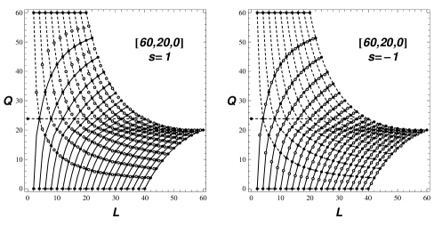
Figure 2: Bohr Somerfield’s quantization of $(L,Q)$ momenta

Appendix: A. SO(2) reduced Poisson bracket
The formulas (11,12,13) determining the bracket $\{.,.\}_{\ast}$ are found considering the following relations

$$d\,[ai]=\begin{cases}\sum_{bcj}\,\epsilon_{abc}\,\,[bi]\,\bar{\gamma}_{cj}(\vec{{\mathsf{L}}},{\mathsf{L}}_{3})\,d{\mathsf{L}}_{j},\\ \sum_{bc}\,\gamma_{abc}\,[bi]\,dL_{c},\end{cases}$$ (128)

$$\bar{\gamma}_{ci}(\vec{x},u)={\hphantom{-}}\delta_{cz}\,f_{1}(\vec{x},u)\,\sum_{a}\epsilon_{im(a)3}\,x_{a}+u^{-1}\,\epsilon_{m(c)i3},$$ (129)

$$\gamma_{ij}(\vec{x},u)=-\delta_{i3}\,\,f_{1}(\vec{x},u)\,\Sigma_{a}\,\epsilon_{jm(a)3}\,x_{a}+u^{-1}\,\epsilon_{ij3},$$ (130)

$$\gamma_{abc}\!=\!\sum_{d}\epsilon_{abd}\,\gamma_{dc}=\sum_{id}\epsilon_{abd}\,\bar{\gamma}_{di}\,[ci],$$ (131)

where $[ai]\!=\![{\rm sign}\,(L_{3})\,\vec{{\mathsf{L}}}\,]_{m(a)i}$, $a,b,\ldots=x,y,z$ and $i,j,\ldots=1,2,3$, $m(x)\!=\!1,\,m(y)\!=\!2,m(z)\!=\!3$ and $\epsilon_{abc}$ is the antisymmetric tensor that $\epsilon_{xyz}\!=\!1$ and $f_{k}(\vec{x},u)=u^{-k}\,(u+x_{z})^{-1}$. Using the above notation and applying Leibnitz rule to formula eq.(12) one finds

$$\sum_{i}\{q^{u}_{a},[ci]\}\,[di]=\Sigma_{bde}\epsilon_{aeb}\,\gamma_{cde}(\vec{l},l_{3})\,q^{u}_{b}=\Sigma_{b}\,\Gamma^{1}_{ab\,cd}(\vec{l},l_{3})\,q^{u}_{b},$$ (132)

$$\sum_{ij}\{[ai],[ci]\}\,[bi]\,[dj]=\sum\gamma_{abe}(\vec{l},l_{3})\,\gamma_{cdf}(\vec{l},l_{3})\,\epsilon_{efg}\,l_{g}=\Gamma^{2}_{ab\,cd}(\vec{l},l_{3}),$$ (133)

$$\Gamma_{ij}(\vec{x},\vec{y},\vec{l},l_{3})=\sum_{kl}x_{k}\,y_{l}\,\sum_{abcd}\,(\Gamma^{1}_{ab\,cd}-\Gamma^{1}_{cd\,ab}+\Gamma^{2}_{ab\,cd})(\vec{l},l_{3})\,[ai]\,[bk]\,[cj][d\,l]$$ (134)

The explicit calculations give

$$\Gamma^{1}_{ab\,cd}(\vec{x},u)=f_{2}(\vec{x},u)\,\sum_{ef}\epsilon_{abe}\,\epsilon_{cdf}\,[\varepsilon_{f}\,(1-\delta_{ez})\,x_{e}\,x_{3-f}+P_{ef}(\vec{x},u)],$$ (135)

$$\Gamma^{2}_{ab\,cd}(\vec{x},u)=f_{1}(\vec{x},u)\,\sum_{efg}\epsilon_{abe}\,\epsilon_{cdf}\,\epsilon_{efg}\,(\epsilon\,x_{g}+\delta_{g3}\,x),$$ (136)

$$P_{ef}(\vec{x},u)=\sum_{g}\epsilon_{efg}\,(u+\delta_{ez}\,x_{e})\,(x_{g}+\delta_{gz}\,u),$$ (137)

where $\varepsilon_{x}\!=\!-\varepsilon_{y}\!=\!1,\,\varepsilon_{z}\!=\!0$ and $\vec{x}=(x_{x},x_{y},x_{z})$. Comparing these formulas with eq.(13) one finds $\Gamma_{ij}(\vec{x},\vec{y},l_{3})=\Gamma_{ij}(\vec{x},\vec{y},\vec{l},l_{3})$; hence, $\gamma^{kl}_{ij}={l_{3}}\,\sum_{abcd}\,(\Gamma^{1}_{ab\,cd}-\Gamma^{1}_{cd\,ab}+\Gamma^{2}_{ab\,cd})(\vec{l},l_{3})\,[ai]\,[bk]\,[cj]\\ \times{[d\,l]}$ which with help of equations (135,136,137) restate the formula eq.(11).

In order to close the system of Poisson relations related with coordinates system $(\boldsymbol{b}^{1},\boldsymbol{b}^{2},\vec{{\mathsf{L}}})$ where $L(A(\boldsymbol{b}^{1},\boldsymbol{b}^{2}))=(0,0,L_{3}\!=\!\pm|\vec{{\mathsf{L}}}|)$ let us write,

$$\{{\mathsf{L}}_{a},b_{iun}\}=h_{aiun}=\,\psi_{a}(\vec{{\mathsf{L}}},L_{3})\,\sum_{j}\,g_{ij}\,b_{jun}.$$ (138)

Since $b_{iun}\!=\!\Sigma_{b}[bi]\,a_{bun}$; hence,

$$h_{aiun}=\Sigma_{bc}\,\epsilon_{abc}\,([bi]\,a_{cun}+\Sigma_{de}\gamma_{deb}\,[ei]\,a_{dun}\,{\mathsf{L}}_{c})=\Sigma_{jk}\,[aj]\,(\epsilon_{jik}+\Sigma_{l}\,\epsilon_{jl3}\,\gamma_{kil}\,L_{3})\,b_{kun},$$ (139)

$$\vec{\psi}(\vec{x},y)={\rm sign}(y)\,\frac{\vec{x}+\vec{e}_{3}\,y}{x_{3}+y},\qquad g_{ij}=\epsilon_{ij3}.$$ (140)

From eq.(116): $\psi_{a}(\vec{{\mathsf{L}}},L_{3})=\partial_{L_{3}}{\mathsf{L}}_{\alpha}=\{\varphi_{L},{\mathsf{L}}_{a}\}$ where we assumed $\{\varphi_{L},p_{L}\}=1,\,p_{L}\!\equiv\!|L_{3}|$. If

$$\mbox{\rsfs L}_{1}\pm i\,\mbox{\rsfs L}_{2}=e^{i\,\varphi_{K}}\,\sqrt{\smash[b]{p_{K}\,(2\,p_{L}-p_{K})}},\qquad\mbox{\rsfs L}_{3}=p_{L}-p_{K},\qquad\{\varphi_{X},p_{Y}\}=\delta_{XY},$$ (141)

where $X,Y\!=\!M,L,K$ then we have too: $\{\varphi_{L},\mbox{\rsfs L}_{\alpha}\}=\partial_{L_{3}}\,\mbox{\rsfs L}_{3}=\psi_{\alpha}(\vec{\mbox{\rsfs L}},L_{3})$ which restate the rules in eq.(111).

References

- 1 M. Cerkaski, J.Math.Phys., 44, 2579–2595 (2003).
- 2 G. Rosensteel and D.J. Rowe, Ann. Phys. (N.Y.) , 198–233 (1980).
- 3 G.Rosensteel and D.J.Rowe, Ann. Phys. (N.Y.) , 343–370 (1980).
- 4 D.J.Rowe, Rep. Prog. Phys. , 1419–1480 (1985).
- 5 M. Cerkaski and I. N. Mikhailov, Ann. Phys. 223,151–179 (1993).
- 6 S. Chandrasekhar, “Ellipsoidal figures of equilibrium,” New Haven and London, Yale University Press, 1969.
- 7 M. Cerkaski and Z. Szymanski, A. Phys. Pol. B 82, 163 (1978).
- 8 A.Bohr, B.R.Mottelson, “Nuclear Structure,” Vol I, W. A. Benjamin, Inc. 1969, New York, Amsterdam.
- 9 A.Bohr, B.R.Mottelson, “Nuclear Structure,” Vol II, W. A. Benjamin, New York 1974, New York, Amsterdam.
- 10 E. R. Marshalek, Nucl.Phys.A 331, 429 (1979).
- 11 R. G. Nazmitdinov and J. Kvasil, JETP 105, 962 (2007).