Meson properties at finite temperature in a three flavor nonlocal chiral quark model with Polyakov loop

Abstract

We study the finite temperature behavior of light scalar and pseudoscalar meson properties in the context of a three-flavor nonlocal chiral quark model. The model includes mixing with active strangeness degrees of freedom, and takes care of the effect of gauge interactions by coupling the quarks with the Polyakov loop. We analyze the chiral restoration and deconfinement transitions, as well as the temperature dependence of meson masses, mixing angles and decay constants. The critical temperature is found to be $T_{c}\simeq 202$ MeV, in better agreement with lattice results than the value recently obtained in the local SU(3) PNJL model. It is seen that above $T_{c}$ pseudoscalar meson masses get increased, becoming degenerate with the masses of their chiral partners. The temperatures at which this matching occurs depend on the strange quark composition of the corresponding mesons. The topological susceptibility shows a sharp decrease after the chiral transition, signalling the vanishing of the U(1)_A anomaly for large temperatures.

I Introduction

The detailed understanding of the behavior of strongly interacting matter under extreme conditions of temperature and/or density has become an issue of great interest in recent years. In this context, it is clearly important to study how hadron properties (masses, mixing angles, decay constants, etc.) get modified when hadrons propagate in a hot and/or dense medium. In particular, since the origin of the light scalar and pseudoscalar mesons is related to the phenomenon of chiral symmetry breaking, the temperature and/or density behavior of their properties is expected to provide relevant information about a possible chiral symmetry restoration. Unfortunately, even if a significant progress has been made on the development of ab initio calculations such as lattice QCD All03 ; Fod04 ; Kar03 , these are not yet able to provide a full understanding of the QCD phase diagram and the related hadron properties, due to the well-known difficulties of dealing with small current quark masses and finite chemical potentials. Thus it is important to develop effective models that show consistency with lattice results and can be extrapolated into regions not accessible by lattice calculation techniques. In previous works GDS00 ; GDS02 ; GDS05 ; DGS04 the study of the phase diagram of SU(2) chiral quark models that include nonlocal interactions Rip97 has been undertaken. These theories can be viewed as nonlocal extensions of the widely studied Nambu$-$Jona-Lasinio model reports . In fact, nonlocality arises naturally in the context of several successful approaches to low-energy quark dynamics as, for example, the instanton liquid model Schafer:1996wv and the Schwinger-Dyson resummation techniques RW94 . Lattice QCD calculations Parappilly:2005ei also indicate that quark interactions should act over a certain range in momentum space. Moreover, several studies BB95 ; BGR02 have shown that nonlocal chiral quark models provide a satisfactory description of hadron properties at zero temperature and density. On the other hand, when looking at the description of the chiral phase transition, it has been noticed that for zero chemical potential these models lead to a rather low critical temperature $T_{c}$ in comparison with lattice results GDS00 ; GDS02 . However, it has been recently shown that the inclusion of the Polyakov loop, which can be taken as an order parameter for the deconfinement transition, leads to a significant increase of the chiral restoration temperature both in two-flavor Blaschke:2007np and three-flavor Contrera:2007wu nonlocal models. The inclusion of the Polyakov loop has also been considered in the context of NJL-like models, namely the so-called PNJL models Meisinger:1995ih ; Fukushima:2003fw ; Megias:2004hj ; Ratti:2005jh ; Roessner:2006xn , and the quark-meson model Schaefer:2009ui .

The aim of the present work is to go one step beyond previous analyses, studying the finite temperature behavior of light scalar and pseudoscalar meson properties in the context of three-flavor nonlocal chiral models that include mixing with active strangeness degrees of freedom, and taking care of the effect of gauge interactions by coupling the quarks with a background color gauge field.

This article in organized as follows. In Sect. II we present the general formalism and derive the expressions needed to evaluate the different meson properties at finite temperature. In Sect. III we provide details concerning the determination of model parameter values as well as the results obtained at zero temperature. Our results for the behavior of the different meson properties as a function of the temperature are presented and discussed in Sect. IV. Finally, in Sect. V we sketch our conclusions.

II The formalism

We deal here with a nonlocal covariant SU(3) quark model which includes the coupling to a background color gauge field. The Euclidean effective action for the quark sector of this model is given by

$$S_{E} = \int d^{4}x\ \left\{\bar{\psi}(x)\left[-i\gamma_{\mu}D_{\mu}+\hat{m}\right]\psi(x)-\frac{G}{2}\left[j_{a}^{S}(x)\ j_{a}^{S}(x)+j_{a}^{P}(x)\ j_{a}^{P}(x)\right]\right.$$ (1)

$$\qquad\qquad\left.-\frac{H}{4}\ T_{abc}\left[j_{a}^{S}(x)j_{b}^{S}(x)j_{c}^{S}(x)-3\ j_{a}^{S}(x)j_{b}^{P}(x)j_{c}^{P}(x)\right]\ +\ {\cal U}\,[A(x)]\right\}\ ,$$

where the chiral U(3) vector $\psi$ includes the light quark fields, $\psi\equiv(u\;d\;s)^{T}$, and $\hat{m}={\rm diag}(m_{u},m_{d},m_{s})$ stands for the current quark mass matrix. For simplicity we consider the isospin symmetry limit, in which $m_{u}=m_{d}=\bar{m}$. The fermion kinetic term includes a covariant derivative $D_{\mu}\equiv\partial_{\mu}-iA_{\mu}$, where $A_{\mu}$ are color gauge fields, and the operator $\gamma_{\mu}\partial_{\mu}$ in Euclidean space is defined as $\sum_{i=1,3}\gamma_{i}\frac{\partial}{\partial x_{i}}+\gamma_{4}\frac{\partial}{\partial\tau}$, with $\gamma_{4}=i\gamma_{0}$. Regarding the interaction terms, the currents $j_{a}^{S,P}(x)$ are given by

$$j_{a}^{S}(x) = \int d^{4}z\ \tilde{g}(z)\ \bar{\psi}\left(x+\frac{z}{2}\right)\ \lambda_{a}\ \psi\left(x-\frac{z}{2}\right)$$ (2)

$$j_{a}^{P}(x) = \int d^{4}z\ \tilde{g}(z)\ \ \bar{\psi}\left(x+\frac{z}{2}\right)\ i\gamma_{5}\lambda_{a}\ \psi\left(x-\frac{z}{2}\right)\ ,$$ (3)

where $\tilde{g}(z)$ is a form factor responsible for the nonlocal character of the interaction, and the matrices $\lambda_{a}$, with $a=0,..,8$, are the standard eight Gell-Mann $3\times 3$ matrices —generators of SU(3)— plus $\lambda_{0}=\sqrt{2/3}\;\openone_{3\times 3}$. The constants $T_{abc}$ in the t’Hooft term (responsible for flavor-mixing) are defined by

$$T_{abc}=\frac{1}{3!}\ \epsilon_{ijk}\ \epsilon_{mnl}\ \left(\lambda_{a}\right)_{im}\left(\lambda_{b}\right)_{jn}\left(\lambda_{c}\right)_{kl}\;.$$ (4)

Finally, the action (1) also includes an effective potential ${\cal U}$ that accounts for gauge field self-interactions.

The partition function associated with the effective action Eq. (1) can be bosonized in the usual way introducing the scalar and pseudoscalar meson fields $\sigma_{a}(x)$ and $\pi_{a}(x)$ respectively, together with auxiliary fields $S_{a}(x)$ and $P_{a}(x)$. To deal with these auxiliary fields we follow the standard stationary phase approximation, which provides a set of equations that relate them to the scalar and pseudoscalar meson fields. Since we are interested in studying the behavior of various meson properties in the presence of a heat bath, we have to extend the bosonized effective action to finite temperature. In the present work this is done by using the Matsubara formalism.

The coupling of fermions to the color gauge fields is implemented through the covariant derivative in the fermion kinetic term $\gamma_{\mu}D_{\mu}$. As usual, we will assume that the quarks move in a constant background field $A_{4}=iA_{0}=ig\,\delta_{\mu 0}\,G^{\mu}_{a}\lambda^{a}/2$, where $G^{\mu}_{a}$ are the SU(3) color gauge fields. Then the traced Polyakov loop, which is taken as order parameter of confinement, is given by $\Phi=\frac{1}{3}{\rm Tr}\,\exp(i\beta\phi)$, where $\beta=1/T$, $\phi=iA_{0}$. We will work in the so-called Polyakov gauge, in which the matrix $\phi$ is given a diagonal representation $\phi=\phi_{3}\lambda_{3}+\phi_{8}\lambda_{8}$, which leaves only two independent variables, $\phi_{3}$ and $\phi_{8}$.

To treat the resulting finite temperature system of interacting mesons in the presence of the Polyakov loop we consider first the mean field approximation (MFA), keeping only the nonzero vacuum expectation values $\bar{\sigma}_{a}$. Note that due to charge conservation only $\bar{\sigma}_{a=0,3,8}$ can be different from zero. Moreover, $\bar{\sigma}_{3}$ also vanishes in the isospin limit. The corresponding MFA grand canonical thermodynamical potential reads

$$\Omega_{\rm MFA}(T) = -\,2\,\sum_{f,c}\int_{p,n}\mbox{ Tr ln}\left[p_{nc}^{2}+\Sigma_{f}^{2}(p_{nc})\right]\;$$ (5)

$$\qquad\qquad-\;\frac{1}{2}\left[\sum_{f}(\bar{\sigma}_{f}\ \bar{S}_{f}+\frac{G}{2}\ \bar{S}_{f}^{2})\;+\;\frac{H}{2}\,\bar{S}_{u}\ \bar{S}_{d}\ \bar{S}_{s}\right]+\;{\cal{U}}(\Phi,T)\ ,$$

where $f=u,d,s$, $c=r,g,b$, and the shorthand notation $\int_{p,n}=\sum_{n}\int d^{3}p/(2\pi)^{3}$ has been used. We have also introduced the definition $p_{nc}=(\vec{p}\ ,\omega_{n}-\phi_{c})$, where $\omega_{n}$ stands for the fermionic Matsubara frequencies and the quantities $\phi_{c}$ are defined by the relation $\phi={\rm diag}(\phi_{r},\phi_{g},\phi_{b})$. The quark constituent masses $\Sigma_{f}(p_{nc})$ are here momentum-dependent quantities, given by

$$\Sigma_{f}(p_{nc})\ =\ m_{f}\,+\,\bar{\sigma}_{f}\,g(p_{nc})\ ,$$ (6)

where $g(p)$ is the Fourier transform of the form factor $\tilde{g}(z)$. For convenience we have introduced mean field values $\bar{\sigma}_{f}$ given by

$$\bar{\sigma}_{u} = \sqrt{\frac{2}{3}}\,\bar{\sigma}_{0}+\bar{\sigma}_{3}+\frac{1}{\sqrt{3}}\,\bar{\sigma}_{8}\;,\quad\bar{\sigma}_{d}=\sqrt{\frac{2}{3}}\,\bar{\sigma}_{0}-\bar{\sigma}_{3}+\frac{1}{\sqrt{3}}\,\bar{\sigma}_{8}\;,\quad\bar{\sigma}_{s}=\sqrt{\frac{2}{3}}\,\bar{\sigma}_{0}+\frac{2}{\sqrt{3}}\,\bar{\sigma}_{8}\;,$$

and similar definitions hold for $\bar{S}_{f}$ in terms of $\bar{S}_{0}$, $\bar{S}_{3}$ and $\bar{S}_{8}$. Note that in the isospin limit $\bar{\sigma}_{u}=\bar{\sigma}_{d}$, thus we have $\Sigma_{u}(p_{nc})=\Sigma_{d}(p_{nc})$. Within the stationary phase approximation, the mean field values of the auxiliary fields $\bar{S}_{f}$ turn out to be related with the mean field values of the scalar fields $\bar{\sigma}_{f}$ by Scarpettini:2003fj

$$\bar{\sigma}_{u}+G\,\bar{S}_{u}+\frac{H}{2}\,\bar{S}_{u}\bar{S}_{s}=0\ \ ,\qquad\bar{\sigma}_{s}+G\,\bar{S}_{s}+\frac{H}{2}\,\bar{S}_{u}^{2}=0\ \ .$$ (7)

The effective potential ${\cal{U}}(\Phi,T)$, which accounts for Polyakov loop dynamics, can be fitted by taking into account group theory constraints together with lattice results, from which one can estimate the temperature dependence. Following Ref. Roessner:2006xn we take

$${\cal{U}}(\Phi,T)=\left[-\,\frac{1}{2}\,a(T)\,\Phi^{2}\;+\;b(T)\,\ln(1-6\,\Phi^{2}+8\,\Phi^{3}-3\,\Phi^{4})\right]T^{4}\ ,$$ (8)

with the corresponding definitions of $a(T)$ and $b(T)$. Owing to the charge conjugation properties of the QCD Lagrangian Dumitru:2005ng , the mean field traced Polyakov loop field $\Phi$ is expected to be a real quantity. Assuming that $\phi_{3}$ and $\phi_{8}$ are real-valued Roessner:2006xn , this implies $\phi_{8}=0$, $\Phi=[2\cos(\phi_{3}/T)+1]/3$.

For finite current quark masses the quark contribution to $\Omega_{\rm MFA}(T)$ turns out to be divergent. To regularize it we follow the same prescription as in previous works GDS05 . Namely, we subtract from $\Omega_{\rm MFA}(T)$ the quark contribution in the absence of fermion interactions, and then we add it in a regularized form, i.e. after the subtraction of an infinite, $T$-independent contribution. From the minimization of this regularized thermodynamical potential it is possible now to obtain a set of three coupled “gap” equations that determine the mean field values $\bar{\sigma}_{u}$, $\bar{\sigma}_{s}$ and $\phi_{3}$ at a given temperature:

$$\frac{\partial\Omega_{\rm MFA}}{\left(\partial\bar{\sigma}_{u},\partial\bar{\sigma}_{s},\partial\phi_{3}\right)}\ =\ 0\ .$$ (9)

In order to obtain the meson mass spectrum and other properties one has to consider the mesonic fluctuations around the mean field values. We begin by introducing a more convenient basis defined by

$$\xi_{ij}=\frac{1}{\sqrt{2}}\,\left(\lambda_{a}\ \xi_{a}\right)_{ij}\;,$$ (10)

where $\xi_{a}=\sigma_{a},\pi_{a}$, while $i,j$ run from 1 to 3 (neutral fields are shifted by $\xi_{a}\to\xi_{a}-\bar{\xi}$). For the scalar fields one has in this way

$$\sigma_{ij}=\left(\begin{array}[]{ccc}\displaystyle\frac{a_{0}^{0}}{\sqrt{2}}+\frac{\sigma_{8}}{\sqrt{6}}+\frac{\sigma_{0}}{\sqrt{3}}&a_{0}^{+}&\kappa^{+}\\ a_{0}^{-}&\displaystyle-\frac{a_{0}^{0}}{\sqrt{2}}+\frac{\sigma_{8}}{\sqrt{6}}+\frac{\sigma_{0}}{\sqrt{3}}&\kappa^{0}\\ \kappa^{-}&\bar{\kappa}^{0}&\displaystyle-\frac{2\,\sigma_{8}}{\sqrt{6}}+\frac{\sigma_{0}}{\sqrt{3}}\end{array}\right)_{ij}\ ,$$ (11)

while a similar expression holds for the pseudoscalar sector, replacing $a_{0}\to\pi$, $\sigma\to\eta$ and $\kappa\to K$. Using this notation the resulting quadratic contribution to the finite temperature bosonized effective action can be written as

$$S_{E}^{\rm quad}=\frac{1}{2}\int_{q,m}\left[G^{+}_{ij,kl}(\vec{q}\ ^{2},\nu_{m}^{2})\ \sigma_{ij}(q_{m})\ \sigma_{kl}(-q_{m})+G^{-}_{ij,kl}(\vec{q}\ ^{2},\nu_{m}^{2})\ \pi_{ij}(q_{m})\ \pi_{kl}(-q_{m})\right]\;,$$ (12)

where $q_{m}=(\vec{q}\ ,\nu_{m})$, $\nu_{m}=2m\pi T$ being bosonic Matsubara frequencies. The functions $G^{\pm}_{ij,kl}$ in Eq. (12) are given by

$$G^{\pm}_{ij,kl}(\vec{q}\ ^{2},\nu_{m}^{2})=C^{\pm}_{ij}(\vec{q}\ ^{2},\nu_{m}^{2})\ \delta_{il}\,\delta_{jk}+\left((r^{\pm})^{-1}\right)_{ij,kl}\;,$$ (13)

where

$$C^{\pm}_{ij}(\vec{q}\ ^{2},\nu_{m}^{2}) = -\,8\,\sum_{c}\,\int_{p,n}\ g(p_{nc}+q_{m}/2)^{2}\ \frac{p_{nc}^{2}+p_{nc}\cdot q_{m}\mp\Sigma_{i}(p_{nc}+q_{m})\Sigma_{j}(p_{nc})}{D_{i}(p_{nc}+q_{m})D_{j}(p_{nc})}\ ,$$ (14)

and

$$r^{\pm}_{ij,kl} = G\ \delta_{il}\,\delta_{jk}\pm\frac{H}{2}\ \epsilon_{ikh}\,\epsilon_{jlh}\ \bar{S}_{h}\ .$$ (15)

In Eq. (14) we have defined $D_{j}(s)\equiv s^{2}+\Sigma_{j}^{2}(s)$, where $j=1,2,3$ correspond to $f=u,d,s$ in the notation of Eq. (6).

From the quadratic effective action $S_{E}^{\rm quad}$ it is possible to derive the scalar and pseudoscalar meson masses as well as the quark-meson couplings. In what follows we will consider explicitly only the case of pseudoscalar mesons. The corresponding expressions for the scalar sector are completely equivalent, just replacing upper indices “$-$” by “$+$”. In terms of the physical fields, the contribution of pseudoscalar mesons to $S_{E}^{\rm quad}$ can be written as

$$\left.S_{E}^{\rm quad}\right|_{P} = \frac{1}{2}\int_{q,m}\,\bigg{\{}G_{\pi}(\vec{q}\ ^{2},\nu_{m}^{2})\left[\pi^{0}(q_{m})\ \pi^{0}(-q_{m})+2\,\pi^{+}(q_{m})\ \pi^{-}(-q_{m})\right]$$ (16)

$$\qquad\qquad+G_{K}(\vec{q}\ ^{2},\nu_{m}^{2})\left[2\,K^{0}(q_{m})\ \bar{K}^{0}(-q_{m})+2\,K^{+}(q_{m})\ K^{-}(-q_{m})\right]$$

$$\qquad\qquad+G_{\eta}(\vec{q}\ ^{2},\nu_{m}^{2})\ \eta(q_{m})\ \eta(-q_{m})+G_{\eta^{\prime}}(\vec{q}\ ^{2},\nu_{m}^{2})\ \eta^{\prime}(q_{m})\ \eta^{\prime}(-q_{m})\bigg{\}}\;.$$

Here, the fields $\eta$ and $\eta^{\prime}$ are related to the U(3) states $\eta_{0}$ and $\eta_{8}$ according to

$$\eta = \cos\theta_{\eta}\ \eta_{8}-\sin\theta_{\eta}\ \eta_{0}$$

$$\eta^{\prime} = \sin\theta_{\eta^{\prime}}\ \eta_{8}+\cos\theta_{\eta^{\prime}}\ \eta_{0}\ ,$$ (17)

where the mixing angles $\theta_{\eta,\eta^{\prime}}$ are defined in such a way that there is no $\eta-\eta^{\prime}$ mixing at the level of the quadratic action. In a similar way, in the scalar sector one has two physical scalar mesons $\sigma$ and $f_{0}(980)$ that are linear combinations of the states $\sigma_{8}$ and $\sigma_{0}$, with mixing angles $\theta_{\sigma}$ and $\theta_{f_{0}}$. The functions $G_{P}(\vec{q}\ ^{2},\nu_{m}^{2})$ introduced in Eq. (16) are given by

$$G_{\pi}(\vec{q}\ ^{2},\nu_{m}^{2})\! \!=\! \!\left[(G+\frac{H}{2}\bar{S}_{s})^{-1}+C^{-}_{uu}(\vec{q}\ ^{2},\nu_{m}^{2})\right]$$

$$G_{K}(\vec{q}\ ^{2},\nu_{m}^{2})\! \!=\! \!\left[(G+\frac{H}{2}\bar{S}_{u})^{-1}+C^{-}_{us}(\vec{q}\ ^{2},\nu_{m}^{2})\right]$$ (18)

$$G_{\eta}(\vec{q}\ ^{2},\nu_{m}^{2})\! \!=\! \!\frac{G^{-}_{88}(\vec{q}\ ^{2},\nu_{m}^{2})+G^{-}_{00}(\vec{q}\ ^{2},\nu_{m}^{2})}{2}-\sqrt{\left[G^{-}_{08}(\vec{q}\ ^{2},\nu_{m}^{2})\right]^{2}\!+\!\left[\frac{G^{-}_{88}(\vec{q}\ ^{2},\nu_{m}^{2})-G^{-}_{00}(\vec{q}\ ^{2},\nu_{m}^{2})}{2}\right]^{2}}$$

$$G_{\eta^{\prime}}(\vec{q}\ ^{2},\nu_{m}^{2})\! \!=\! \!\frac{G^{-}_{88}(\vec{q}\ ^{2},\nu_{m}^{2})+G^{-}_{00}(\vec{q}\ ^{2},\nu_{m}^{2})}{2}+\sqrt{\left[G^{-}_{08}(\vec{q}\ ^{2},\nu_{m}^{2})\right]^{2}\!+\!\left[\frac{G^{-}_{88}(\vec{q}\ ^{2},\nu_{m}^{2})-G^{-}_{00}(\vec{q}\ ^{2},\nu_{m}^{2})}{2}\right]^{2}}\;,$$

where

$$G^{-}_{88}(\vec{q}\ ^{2},\nu_{m}^{2}) = \frac{1}{3}\frac{6G-4H\bar{S}_{u}-2H\bar{S}_{s}}{2G^{2}-GH\bar{S}_{s}-H^{2}\bar{S}_{u}^{2}}+C^{-}_{88}(\vec{q}\ ^{2},\nu_{m}^{2})$$

$$G^{-}_{08}(\vec{q}\ ^{2},\nu_{m}^{2}) = \frac{\sqrt{2}}{3}\frac{H(\bar{S}_{s}-\bar{S}_{u})}{2G^{2}-GH\bar{S}_{s}-H^{2}\bar{S}_{u}^{2}}+C^{-}_{08}(\vec{q}\ ^{2},\nu_{m}^{2})$$ (19)

$$G^{-}_{00}(\vec{q}\ ^{2},\nu_{m}^{2}) = \frac{1}{3}\frac{6G+4H\bar{S}_{u}-H\bar{S}_{s}}{2G^{2}-GH\bar{S}_{s}-H^{2}\bar{S}_{u}^{2}}+C^{-}_{00}(\vec{q}\ ^{2},\nu_{m}^{2})\,.$$

and

$$C^{-}_{88}=\frac{C^{-}_{uu}+2\,C^{-}_{ss}}{3}\ ,\qquad C^{-}_{08}=\frac{\sqrt{2}}{3}\left(C^{-}_{uu}-C^{-}_{ss}\right)\ ,\qquad C^{-}_{00}=\frac{2\,C^{-}_{uu}+C^{-}_{ss}}{3}\ .$$ (20)

Now the pseudoscalar meson masses are obtained by solving the equations

$$G_{P}(-m_{P}^{2},0)=0\;,$$ (21)

with $P=\pi$, $K$, $\eta$ and $\eta^{\prime}$. The mass values determined by these equations correspond to the spatial “screening-masses” of the mesons’ zeroth Matsubara modes, and their inverses describe the persistence lengths of these modes at equilibrium with the heat bath. It is worth to notice that there is a screening mass for each Matsubara mode. The full bound state propagator can be calculated via any polarization tensor that receives a contribution from the bound state, but only once all screening masses have been determined. The propagator obtained in this way is defined only on a discrete set of points along what might be called the imaginary-energy axis, and the “pole-mass”, i.e., the mass that yields the bound state energy pole for $\vec{q}\sim 0$, is obtained only after an analytic continuation of the propagator onto the real-energy axis. The fact that Lorentz invariance is broken for $T>0$ means that, in general, the pole mass and screening masses are not equal (see e.g. Ref. Florkowski:1993br ). Although the analytic continuation involved in this process is not unique, an unambiguous result is obtained by requiring that it yields a function that is bounded at complex-infinity and analytic off the real axis LW87 . From this description it is nonetheless clear that the screening masses completely specify the properties of $T>0$ bound states. The masses associated to the zeroth Matsubara mode studied here are spatial screening masses corresponding to a behavior $\exp(-m_{P}\,r)$ in the conjugate 3-space coordinate $r$, and should correspond to the lowest state in each meson channel. In fact, these are the quantities usually studied in lattice calculations Karsch:2003jg .

In the $\eta-\eta^{\prime}$ system, once the meson masses have been determined one can find the mixing angles $\theta_{\eta}$ and $\theta_{\eta^{\prime}}$, which are in general different from each other. These are given by

$$\mbox{tan}\ 2\,\theta_{P} = \frac{2\,G^{-}_{08}(-m^{2}_{P},0)}{G^{-}_{00}(-m^{2}_{P},0)-G^{-}_{88}(-m^{2}_{P},0)}\ \ ,\qquad P\ =\ \eta,\ \eta^{\prime}\ .$$ (22)

The meson fields have to be renormalized, so that the residues of the corresponding propagators at the meson poles are set equal to one. The corresponding wave function renormalization constants $Z_{P}$ are given by

$$Z_{P}^{-1}=\frac{dG_{P}(\vec{q}\ ^{2},0)}{d\vec{q}\ \!^{2}}\bigg{|}_{\ \vec{q}\ \!^{2}=-m_{P}^{2}}\;,$$ (23)

with $P=\pi$, $K$, $\eta$ and $\eta^{\prime}$. Finally, the meson-quark coupling constants $G_{Pq}$ are given by the original residues of the meson propagators at the corresponding poles,

$$G_{Pq}=Z^{1/2}_{P}\;.$$ (24)

In the case of the pseudoscalar mesons other important features are the corresponding weak decay constants $f_{ab}$, defined by

$$\langle\,0|A^{a}_{\mu}(0)|\pi_{b}(q)\,\rangle=i\;f_{ab}\;q_{\mu}\;.$$ (25)

where $A^{a}_{\mu}$ is the $a$-component of the axial current. For $a,b=1\dots 7$, the constants $f_{ab}$ can be written as $\delta_{ab}\,f_{P}$, with $P=\pi$ for $a=1,2,3$ and $P=K$ for $a=4$ to 7. In contrast, as occurs with the meson masses, the decay constants become mixed in the $a=0,8$ sector. Details on how to obtain the expressions for the axial currents in the presence of nonlocal fields can be found e.g. in Refs. BB95 ; Scarpettini:2003fj . After a rather lengthy calculation we find that, at finite temperature, the pion and kaon decay constants are given by

$$f_{\pi} = 4\,f_{uu}(-m_{\pi}^{2},0)\ Z_{\pi}^{1/2}\;,$$

$$f_{K} = 2\left[f_{us}(-m_{K}^{2},0)+f_{su}(-m_{K}^{2},0)\right]Z_{K}^{1/2}\;,$$ (26)

where

$$f_{ij}(\vec{q}\ \!^{2},\nu_{m}) = \sum_{c}\,\int_{p,n}\Bigg{\{}g\left(p_{nc}+\frac{q_{m}}{2}\right)\frac{p_{nc}\cdot q_{m}\Sigma_{i}(p_{nc}+q_{m})-(p_{nc}\cdot q_{m}+p_{nc}^{2})\Sigma_{j}(p_{nc})}{D_{i}(p_{nc}+q_{m})D_{j}(p_{nc})}$$ (27)

$$\qquad-\left[2g\left(p_{nc}+\frac{q_{m}}{2}\right)-g\left(p_{nc}\right)-g\left(p_{nc}+q_{m}\right)\right]\frac{\Sigma_{i}(p_{nc}+\frac{q_{m}}{2})}{D_{i}(p_{nc}+\frac{q_{m}}{2})}$$

$$\qquad+\ g\left(p_{nc}+\frac{q_{m}}{2}\right)\left[\Sigma_{i}\left(p_{nc}+\frac{q_{m}}{2}\right)+\Sigma_{j}\left(p_{nc}+\frac{q_{m}}{2}\right)-\Sigma_{i}\left(p_{nc}\right)-\Sigma_{j}\left(p_{nc}+q_{m}\right)\right]$$

$$\qquad\qquad\times\;\frac{p_{nc}^{2}+p_{nc}\cdot q_{m}+\Sigma_{i}(p_{nc}+q_{m})\Sigma_{j}(p_{nc})}{D_{i}(p_{nc}+q_{m})D_{j}(p_{nc})}\Bigg{\}}\;.$$

In the case of the $\eta-\eta^{\prime}$ system, two decay constants can be defined for each component ($a=0$ or 8) of the axial current. They can be written in terms of the decay constants $f_{ab}$ and the previously defined mixing angles $\theta_{\eta,\eta^{\prime}}$ as

$$f^{a}_{\eta} = \left[f_{a8}(-m_{\eta}^{2},0)\cos\theta_{\eta}-f_{a0}(-m_{\eta}^{2},0)\sin\theta_{\eta}\right]\ Z_{\eta}^{1/2}$$

$$f^{a}_{\eta^{\prime}} = \left[f_{a8}(-m_{\eta^{\prime}}^{2},0)\sin\theta_{\eta^{\prime}}+f_{a0}(-m_{\eta^{\prime}}^{2},0)\cos\theta_{\eta^{\prime}}\right]\ Z_{\eta^{\prime}}^{1/2}\;.$$ (28)

Within our model, the decay constants $f_{ab}$ for $a,b=0,8$ are related to the $f_{ij}$ defined in Eq. (27) by

$$f_{88}(\vec{q}\ \!^{2},\nu_{m}) = \frac{4}{3}\left[2f_{ss}(\vec{q}\ \!^{2},\nu_{m})+f_{uu}(\vec{q}\ \!^{2},\nu_{m})\right]$$

$$f_{00}(\vec{q}\ \!^{2},\nu_{m}) = \frac{4}{3}\left[2f_{uu}(\vec{q}\ \!^{2},\nu_{m})+f_{ss}(\vec{q}\ \!^{2},\nu_{m})\right]$$ (29)

$$f_{08}(\vec{q}\ \!^{2},\nu_{m})=f_{80}(\vec{q}\ \!^{2},\nu_{m}) = \frac{4\sqrt{2}}{3}\left[f_{uu}(\vec{q}\ \!^{2},\nu_{m})-f_{ss}(\vec{q}\ \!^{2},\nu_{m})\right]\;.$$

As expected, both the nondiagonal decay constants $f_{08}$, $f_{80}$ and the mixing angles $\theta_{\eta}$, $\theta_{\eta^{\prime}}$ vanish in the SU(3) symmetry limit.

III Model parameters and zero temperature results

In this section we determine the model parameters to be used in our numerical calculations, and quote the results obtained for various meson properties at zero temperature. The latter include the values of meson masses, decay constants and mixing angles, as well as quark constituent masses, quark condensates and quark-meson couplings.

At low temperatures, the value of the traced Polyakov loop is essentially determined by the effective potential in Eq. (8), therefore for $T\to 0$ one has $\Phi\to 0$, $\cos(\phi_{3}/T)\to-1/2$. Since for low $T$ the Matsubara sums in the thermodynamical potential are governed by modes with large $n$, one has $\omega_{n}-\phi_{c}=[(2n+1)\pi-\phi_{c}/T]T\simeq\omega_{n}$, thus for $T\to 0$ the coupling of fermions to the Polyakov loop vanishes. In this way, the zero-$T$ calculations are similar to those carried out in Ref. Scarpettini:2003fj , in which SU(3) nonlocal chiral quark models without the inclusion of the Polyakov loop have been considered. As in that work, our numerical analysis has been performed using a Gaussian form factor, namely

$$g(p)\ =\ \exp{\left(-p^{2}/\Lambda^{2}\right)}\ ,$$ (30)

which has been often considered in the literature. This introduces a new free parameter $\Lambda$, which plays the rôle of an ultraviolet cut-off momentum scale (we recall that the form factor is defined in Euclidean momentum space). At $T=0$, the main difference between our analysis and that in Ref. Scarpettini:2003fj is that here we are considering an OGE-motivated nonlocal interaction, whereas in the previous work a different form [motivated by instanton liquid models (ILM)] for the nonlocal currents has been chosen. In the case of two-flavor models, a detailed comparison between these different interaction forms has been carried out in Ref. GomezDumm:2006vz , showing that the results for both models are qualitatively similar. Notice that in Ref. Scarpettini:2003fj only the pseudoscalar meson sector was addressed.

After the assumption of the form factor in Eq. (30), the nonlocal chiral quark model under consideration includes five free parameters, namely the current quark masses $\bar{m}$ and $m_{s}$, the coupling constants $G$ and $H$ and the cut-off scale $\Lambda$. In our numerical calculations we have chosen to fix the value of $\bar{m}$, whereas the remaining four parameters are determined by requiring that the model reproduces correctly the measured values of four physical quantities at zero temperature. These are the masses of the pion, kaon and $\eta^{\prime}$ pseudoscalar mesons, and the pion decay constant $f_{\pi}$. Taking $\bar{m}=5$ MeV, we obtain the following set of parameters:

$$\bar{m} = 5\ {\rm MeV}\ \ {\rm(input)}$$

$$m_{s} = 119\ {\rm MeV}$$

$$\Lambda = 843\ {\rm MeV}$$

$$G\Lambda^{2} = 13.35$$

$$H\Lambda^{5} = -273.7\ \$$ (31)

Our numerical results are presented in Table I. For comparison, in the last column of this table we quote the measured values of meson masses, and the ranges in which the decay constants and mixing angles should fall according to most popular phenomenological approaches. Entries marked with an asterisk are those that we have taken as input values to fix the model parameters. From Table I it is seen that in general there is a reasonable agreement between the predicted meson masses and the empirical values quoted by the Review of Particle Physics PDG2008 . In addition, the obtained mass ratio $m_{s}/m=23.8$ is close to the corresponding current algebra prediction, namely $m_{s}/m=(2m_{K}^{2}-m_{\pi}^{2})/m_{\pi}^{2}\simeq 25$. We point out that in the case of the mass of the $\kappa$ scalar meson the equation $G_{\kappa}(-x^{2},0)=0$ has no solution in the real $x$ axis. Hence we have defined the mass $m_{\kappa}$ as the point where the absolute value of $G_{\kappa}(-x^{2},0)$ becomes minimal. A more sophisticated definition could be done by extending $x$ to the complex plane, thus introducing a finite $\kappa$ width. In any case, this would not change significantly the mass value. A detailed analysis of the regularization prescriptions for the evaluation of loop integrals like those in Eqs. (14) and (27) has been carried out in Ref. Scarpettini:2003fj .

		Our Model		$\begin{array}[]{c}{\rm Empirical\ \&}\\ {\rm Phenomenological}\end{array}$
$\bar{m}$	[ MeV ]	$5^{*}$		(3.4 - 7.4)
$m_{s}$	[ MeV ]	119		(108 - 209)
$m_{\pi}$	[ MeV ]	$139^{*}$		139
$m_{K}$	[ MeV ]	$495^{*}$		495
$m_{\eta}$	[ MeV ]	523		547
$m_{\eta^{\prime}}$	[ MeV ]	$958^{*}$		958
$m_{a_{0}}$	[ MeV ]	900		980
$m_{\kappa}$	[ MeV ]	1380		1425
$m_{\sigma}$	[ MeV ]	566		400-1200
$m_{f_{0}}$	[ MeV ]	1280		980
$G_{\pi q}$		3.98
$G_{Kq}$		4.30
$G_{\eta q}$		3.93
$G_{\eta^{\prime}q}$		2.83
$\theta_{\eta}$		$-2.3^{\circ}$
$\theta_{\eta^{\prime}}$		$-40.3^{\circ}$
$\theta_{8}$		$-24^{\circ}$		$-$($22^{\circ}$ - $19^{\circ}$)
$\theta_{0}$		$-7.7^{\circ}$		$-$($10^{\circ}$ - $0^{\circ}$)
$f_{\pi}$	[ MeV ]	$92.4^{*}$​​​		92.4
$f_{K}/f_{\pi}$		1.17		1.22
$f_{\eta}^{8}/f_{\pi}$		1.14		(1.17-1.22)
$f_{\eta}^{0}/f_{\pi}$		0.16		(0.11-0.37)
$f_{\eta^{\prime}}^{8}/f_{\pi}$		-0.49		-(0.42-0.46)
$f_{\eta^{\prime}}^{0}/f_{\pi}$		1.16		(0.98-1.16)
(*) Input values

Table 1: $T=0$ model predictions for various meson properties: masses, mixing angles, decay constants and quark-meson couplings.

Concerning the pseudoscalar meson decay constants, we notice that the predicted value for $f_{K}$ is also phenomenologically acceptable. In fact, it turns out to be significantly better than that obtained in the standard NJL model, where the kaon and pion decay constants are found to be approximately equal to each other reports in contrast with experimental evidence. Regarding the mixing angles and decay constants for the $\eta_{8}-\eta_{0}$ system, the problem of defining and (indirectly) fitting these parameters has been revisited several times in the literature (see e.g. Ref. F00 , and references therein). As stated in the previous section, in general one has to deal with two different state mixing angles $\theta_{P}$ and four decay constants $f_{P}^{a}$, where $P=\eta,\eta^{\prime}$ and $a=0,8$. This means that $\eta$ and $\eta^{\prime}$ states do not need to be orthogonal, and the same occurs with $(f_{\eta}^{8},f_{\eta^{\prime}}^{8})$ and $(f_{\eta}^{0},f_{\eta^{\prime}}^{0})$ L97 ; FK02 ; EF99 . For the sake of comparison with phenomenological values of these parameters, we follow here Ref. L97 and express the four decays constants $f_{P}^{a}$ in terms of two decay constants $f_{a}$ and two mixing angles $\theta_{a}$, where $a=0,8$:

$$\left(\begin{array}[]{cc}f_{\eta}^{8}&f_{\eta}^{0}\\ f_{\eta^{\prime}}^{8}&f_{\eta^{\prime}}^{0}\end{array}\right)=\left(\begin{array}[]{cc}f_{8}\,\cos\theta_{8}&-f_{0}\,\sin\theta_{0}\\ f_{8}\,\sin\theta_{8}&\ \ f_{0}\,\cos\theta_{0}\end{array}\right)\ .$$ (32)

In our framework the decay constants $f_{P}^{a}$ can be calculated from Eqs. (28). As shown in Table I, both the values obtained for $\theta_{8}$, $\theta_{0}$ as well as those obtained for the decay constants in the $\eta-\eta^{\prime}$ sector are in agreement with phenomenological results. These have been taken from the analysis in Ref. F00 , in which the values obtained from different parameterizations have been translated to the four-parameter decay constant scheme given by Eq. (32). Notice that $\theta_{8}$ and $\theta_{0}$ are significantly different to each other, as occurs with the mixing angles $\theta_{\eta}$ and $\theta_{\eta^{\prime}}$ [which can be calculated from Eq. (22)]. This is in agreement with the analysis in Ref. L97 , carried out within next-to-leading order Chiral Perturbation Theory and large $N_{C}$, which leads to $\theta_{8}=-20.5^{\circ}$, $\theta_{0}=-4^{\circ}$.

IV Finite temperature results

Taking the parameters in Eq. (31), one can solve Eqs. (9) to calculate the mean field values $\bar{\sigma}_{u}$, $\bar{\sigma}_{s}$ and $\phi_{3}$ at finite temperature. The behavior of effective quark masses and condensates, as well as the curves for the traced Polyakov loop $\Phi$, are similar to those obtained in Ref. Contrera:2007wu within an ILM-motivated nonlocal chiral model. The discussion of those results is qualitatively the same as in our case, therefore it will not be repeated here. We just state that, as expected, there is a crossover phase transition in which chiral symmetry is restored, and consequently one finds a sharp peak in the chiral susceptibility. The transition temperature (defined as the position of this peak) is found to be $T_{c}=202$ MeV. This value is in much better agreement with lattice results, $T_{c}^{\rm(latt)}=160-200$ MeV Bernard:2004je , than the value recently obtained in the local SU(3) PNJL model, $T^{\rm(PNJL)}_{c}=259$ MeV Costa:2008dp . In addition one finds a deconfinement phase transition, which occurs at about the same critical temperature.

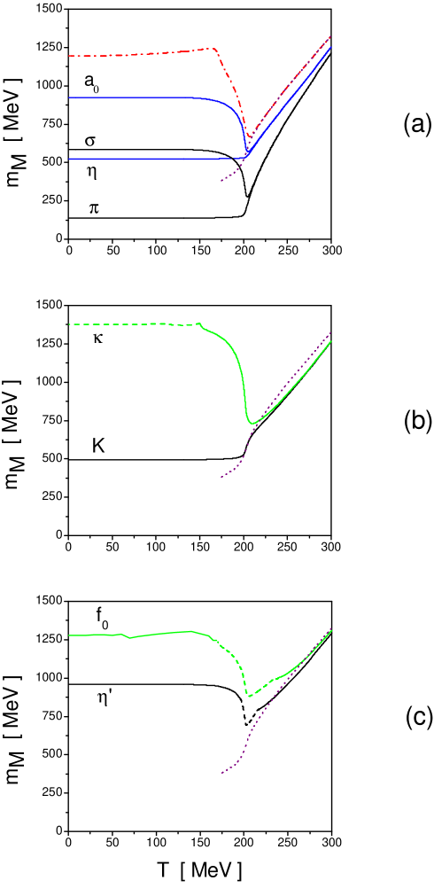
Figure 1: Solid lines quote scalar and pseudoscalar meson masses as functions of the temperature. Dotted and dashed-dotted lines stand for the value $m_{M}^{\rm uq}=2(\pi T-\phi_{3})$ and the $\bar{q}q$ production threshold, respectively (see text).

We concentrate here in the evolution of meson masses and decay constants with temperature, which has not been previously addressed in the context of SU(3) nonlocal models. Pseudoscalar meson masses can be determined by solving Eqs. (21), while the same procedure applies to the scalar meson sector replacing upper indices “$-$ by “$+$” in Eqs. (II-19). As discussed in Sect. II, these values correspond to the spatial screening-masses of the mesons’ zeroth Matsubara modes. Our numerical results are shown in Fig. 1, where we quote the values of meson masses as functions of the temperature. In Fig. 1(a) we show the behavior of the pseudoscalar mesons $\pi$ and $\eta$ together with the curves for the scalar mesons $\sigma$ and $a_{0}$, which are chiral partners of the former. It is seen that pseudoscalar meson masses remain approximately constant up to the critical temperature (this is reasonable, since they are protected from chiral symmetry), while scalar meson masses begin to drop at about 150 MeV. Above $T_{c}$ pseudoscalar masses get increased, in such a way that they become degenerate with the masses of their chiral partners, as expected from chiral restoration. In particular, the fact that this occurs right after the transition in the case of the $(\eta,a_{0})$ pair indicates that the strange contents of the $\eta$ and $a_{0}$ mesons become suppressed above the critical temperature. When the temperature is further increased, all four masses are found to rise continuously, showing that now the mass is basically dominated by thermal energy. At very large temperatures the curves should approach asymptotically the value corresponding to a $q\bar{q}$ pair of uncorrelated massless quarks $m_{M}^{\rm uq}=2\pi T$ Eletsky:1988an . At $T\approx 300$ MeV, however, the Polyakov loop has not yet reached its asymptotic value $\phi_{3}/T|_{T\rightarrow\infty}=0$, and it still provides a non-negligible correction to the quark screening mass. In fact, we find $\phi_{3}/T|_{T=300}\simeq 0.93$. Thus, around this temperature we expect $m_{M}^{\rm uq}=2(\pi T-\phi_{3})$, which is shown by the dotted lines in Figs. 1(a), (b) and (c). For vanishing quark dynamical masses, this value of $m_{M}$ corresponds to a pole in the $n=0$ mode for the integrals in the functions $C_{ii}^{\pm}(-k^{2},0)$, see Eq. (14). Indeed, as discussed in Ref. Blaschke:2000gd , Eqs. (21) can be satisfied only in the vicinities of these poles. On the other hand, in general it is seen that the functions $C_{ij}^{\pm}(-k^{2},0)$ [and therefore also the functions $G_{M}(-k^{2},0)$] are well defined for low values of $k$. If $k$ is increased, at some critical point $k_{\rm crit}$, usually called “pinch point”, the integrals become divergent and need some regularization prescription. In the present work we follow the prescription discussed in the Appendix of Ref. Scarpettini:2003fj , conveniently extended to the finite temperature case. The pinch point occurs when both effective quarks are simultaneously on-shell, thus it can be interpreted as a threshold above which mesons could decay into two massive quarks. In Fig. 1(a) this threshold is represented with the dashed-dotted curve (above $T_{c}$, it approximately matches the value of $m_{M}^{\rm uq}$ mentioned previously). It can be seen that all four meson masses in Fig. 1(a) remain below the threshold for the temperature range considered.

In Fig. 1(b) we represent the curves for the masses of the pseudoscalar mesons $K$, and their scalar partners $\kappa$. It is seen that for some temperature range the equation $G_{\kappa}(-k^{2},0)=0$ has no solution for real $k$, therefore the mass is defined as the minimum of the function $G_{\kappa}(-k^{2},0)$, as discussed in the previous section. These mass values correspond to the dashed stretch of the corresponding curve. It is worth to notice that the $K$ and $\kappa$ meson masses match only at $T\simeq 225$ MeV, i.e. at a temperature somewhat larger than $T_{c}$. This is clearly a consequence of the large current strange quark mass, which is expected to move the SU(3) chiral restoration to higher temperatures. Finally, in Fig. 1(c) we quote the temperature dependence of f₀ and $\eta^{\prime}$ masses. As before, dashed stretches in the curves indicate the regions in which the corresponding function $G_{M}(-k^{2},0)$ has no zero for real $k$ and, therefore, the mass $m_{M}$ is defined by the position of its minimum. Let us first focus on the behavior of the $\eta^{\prime}$ mass. In contrast with some results found in Ref. Horvatic:2007qs , where the corresponding temperature dependence has been studied in the framework of a Dyson-Schwinger approach, we do not observe any kind of enhancement of $m_{\eta^{\prime}}$ around $T_{c}$. It should be noticed that in the framework of Ref. Horvatic:2007qs the effect of the U(1)_A anomaly is modelled in a simpler way, namely by considering it only at the level of mass shifts. In this sense our result is consistent with the analyses of the $\eta^{\prime}$ pole mass performed within the local SU(3) PNJL model Costa:2008dp and the quark-meson model Schaefer:2008hk , where no enhancement was found either. Concerning the degeneracy of $\eta^{\prime}$ with its chiral partner f₀, we see that such a degeneracy is achieved only at $T\simeq 300$ MeV. This a consequence of the strange quark contents of these mesons, which, as we will see below, become larger as the temperature increases.

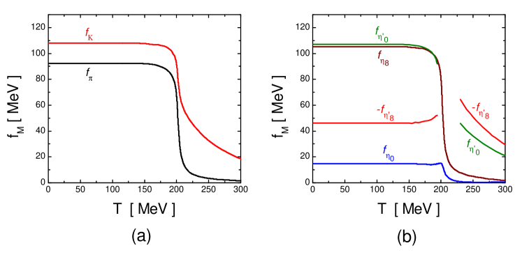
Figure 2: Behavior of pseudoscalar meson decay constants as functions of the temperature.

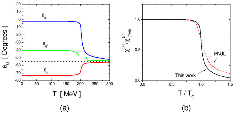
Figure 3: (a) Behavior of meson mixing angles as functions of the temperature. The dashed line shows the “ideal” mixing angle $\theta_{\rm ideal}=\tan^{-1}\sqrt{2}$. (b) Behavior of the topological susceptibility relative to its $T=0$ value as function of the temperature in the nonlocal model (solid) and in the PNJL SU(3) model Costa:2008dp  (dotted).

Figure 4: Behavior of quark-meson couplings as functions of the temperature.

Next, in Fig. 2 we quote the behavior of pseudoscalar meson decay constants, which can be calculated from Eqs. (II), (26) and (28). Fig. 2(a) shows the curves corresponding to the decay constants $f_{\pi}$ and $f_{K}$. It is seen that both decay constants drop at the phase transition. We observe, however, that due to the strange quark content of the kaon the corresponding decay constant shows a slower decrease after the transition. The behavior of the decay constants associated with $\eta-\eta^{\prime}$ system is shown in Fig. 2(b). In the case of $f_{\eta_{0}}$ and $f_{\eta_{8}}$ such a behavior is similar to that of $f_{\pi}$, while the decrease after the transition is less pronounced for $f_{\eta^{\prime}_{0,8}}$. Again, this behaviour of the $\eta^{\prime}$ decay constants can be understood in terms of its larger strange quark content. Here we have left blank the range in which the $\eta^{\prime}$ mass is not well defined.

In Fig. 3(a) we plot the behavior of the mixing angles $\theta_{\eta}$ and $\theta_{\eta^{\prime}}$, which can be calculated from Eq. (22). It is seen that above the phase transition both angles tend to a common value, which is natural since meson masses also tend to unify. More interestingly, they converge to the so-called “ideal” mixing angle $\theta_{\rm ideal}=\tan^{-1}\sqrt{2}\simeq 54.7^{\circ}$ (dashed line in the figure). This means that, as suggested above, the $\eta$ meson becomes approximately non-strange, while $\eta^{\prime}$ approaches to an $\bar{s}s$ pair. The same happens with the $\sigma-{\rm f}_{0}$ pair (in the figure we have quoted only $\theta_{\sigma}$, since the f₀ meson mass lies above the $\bar{q}q$ threshold). The fact that the mixing angles go to the “ideal” value for large temperatures implies that the U(1)_A anomaly tends to vanish in this limit. Another signature of this fact is that axial chiral partners $(\pi,\eta)$ and $(\sigma,a_{0})$ become almost degenerate at $T\simeq 300$ MeV. However, perhaps the best indication of the vanishing of the U(1)_A anomaly is provided by the topological susceptibility $\chi$ which, in pure color SU(3) theory, is related to the $\eta^{\prime}$, $\eta$ and $K$ masses through the Witten-Veneziano formula

$$\frac{6}{f_{\pi}^{2}}\ \chi\ =\ m_{\eta^{\prime}}^{2}+m_{\eta}^{2}-2m_{K}^{2}\ .$$ (33)

Various existing lattice calculations Alles:1996nm show a sharp decrease of $\chi$ at the critical temperature. In our framework, the topological susceptibility can be calculated from

$$\!\!\!\!\!\!\!\!\!\!\chi = -\frac{H^{2}}{8}\left\{2\,C^{-}_{uu}\bar{S}_{u}^{2}\bar{S}_{s}^{2}\,+C^{-}_{ss}\bar{S}_{u}^{4}\,-\,\frac{2}{3}\left[\frac{\bar{S}_{u}(\bar{S}_{u}+2\bar{S}_{s})}{\sqrt{2}}\left(\begin{array}[]{c}C^{-}_{08}\\ C^{-}_{00}\\ \end{array}\right)^{\dagger}+\bar{S}_{u}(\bar{S}_{s}-\bar{S}_{u})\left(\begin{array}[]{c}C^{-}_{88}\\ C^{-}_{80}\\ \end{array}\right)^{\dagger}\right]\right.$$ (43)

$$\left.\qquad\qquad\qquad\qquad\qquad\cdot\;{\cal G}^{-1}\;\cdot\,\left[\frac{\bar{S}_{u}(\bar{S}_{u}+2\bar{S}_{s})}{\sqrt{2}}\left(\begin{array}[]{c}C^{-}_{08}\\ C^{-}_{00}\\ \end{array}\right)+\bar{S}_{u}(\bar{S}_{s}-\bar{S}_{u})\left(\begin{array}[]{c}C^{-}_{88}\\ C^{-}_{80}\\ \end{array}\right)\right]\right\}\ ,$$

where ${\cal G}$ is a $2\times 2$ matrix whose matrix elements are given in Eq. (19), and all functions are evaluated at $(\vec{q}\ ^{2},\nu_{m}^{2})=(0,0)$. This expression has been obtained following similar steps as those described in Ref. Fukushima:2001hr for the case of the (local) NJL model. The numerical results are shown in Fig. 3(b). To be able to compare with the result obtained in the local PNJL SU(3) model Costa:2008dp (where, as already mentioned, $T_{c}$ turns out to be too high), we show the normalized value of $\chi^{1/4}$ as a function of $T/T_{c}$. For both models one finds a sharp decrease in the topological susceptibility at the critical temperature, this decrease being steeper in the nonlocal model. Indeed, at $T/T_{c}=1.5$ the ratio $\chi^{1/4}/\chi_{(T=0)}^{1/4}$ is about 11% for the local PNJL model, while for the nonlocal model it is roughly one half of this value. The value of $\chi_{(T=0)}^{1/4}$ is found to be about 162 MeV in the nonlocal model, while one gets $\simeq 180$ MeV in the PNJL. Recent lattice calculations (see Ref. Durr:2006ky and references therein) indicate that $\chi_{(T=0)}^{1/4}\simeq 190$ MeV in pure gauge theories. However, light dynamical quarks are expected to suppress the topological susceptibility AliKhan:2001ym . For example, in the lattice calculation carried out in Ref. Alles:2000cg the authors find $\chi_{(T=0)}^{1/4}\simeq 163$ MeV for a two-flavor case in the region where the current quark masses are around 20 MeV.

For completeness, we conclude our description by quoting in Fig. 4 the behavior of the quark-meson couplings $G_{Mq}$. These can be calculated from Eqs. (23) and (24) for pseudoscalar mesons, and similar relations hold for the scalar meson sector with the appropriate changes in the functions $C_{ij}(\vec{q}\ ^{2},0)$.

V Summary and conclusions

In the present work we have studied the finite temperature behavior of light scalar and pseudoscalar meson properties in the context of three-flavor nonlocal chiral models that include mixing with active strangeness degrees of freedom. The effect of gauge interactions has been introduced by coupling the quarks with a background gauge field, and the deconfinement transition has been studied through the behavior of the traced Polyakov loop. For a given parameterization of the nonlocality —which, for simplicity, here is introduced through an exponential form factor—, at zero temperature the model has five free parameters. We have chosen to fix the average non-strange quark mass $\bar{m}$ to a phenomenologically sound value of $\bar{m}=5$ MeV, whereas the remaining four parameters have been determined by requiring that the model reproduces correctly the measured values of the masses of the pion, kaon and $\eta^{\prime}$ pseudoscalar mesons, and the pion decay constant $f_{\pi}$. Using this set of parameters one can obtain a very good description of the remaining zero temperature pseudoscalar meson properties, as well as adequate values for the scalar meson masses.

In the extension to finite temperature the former parameter values have been kept fixed, while those appearing in the Polyakov loop potential have been taken from a fit to lattice results. As expected, the model shows a fast crossover phase transition, corresponding to the restoration of SU(2) chiral symmetry. The transition temperature (defined as the position of the peak of the corresponding chiral susceptibility) is found to be $T_{c}=202$ MeV. This value is in better agreement with lattice results, namely $T_{c}^{\rm(latt)}=160-200$ MeV Bernard:2004je , than the value recently obtained in the local SU(3) PNJL model, $T^{(\rm PNJL)}_{c}=259$ MeV Costa:2008dp . In addition one finds a deconfinement phase transition, which occurs at about the same critical temperature. Concerning the behavior of meson masses with temperature, it is seen that pseudoscalar meson masses remain approximately constant up to $T_{c}$, while scalar meson masses begin to drop at about 150 MeV. Beyond $T_{c}$ pseudoscalar masses get increased, in such a way that they become degenerate with the masses of their chiral partners, as expected from chiral restoration. The temperature at which chiral partners meet depend on the strange quark composition of the corresponding mesons, i.e. the masses of mesons containing no strange quarks match almost immediately after $T_{c}$, while f₀ and $\eta^{\prime}$ masses meet only at about 1.5 $T_{c}$, the situation being intermediate for K and $\kappa$ mesons. Regarding the properties of the $\eta-\eta^{\prime}$ sector, it is seen that the corresponding mixing angles tend to converge to the so-called “ideal” mixing, which indicates that the U(1)_A anomaly tends to vanish as the temperature increases. This is also seen in the behavior of the topological susceptibility which, as expected from lattice calculations, shows a sharp decrease after the chiral phase transition. It should be noticed, however, that in the present nonlocal model such a decrease is faster than that obtained in the local PNJL SU(3) Costa:2008dp . Finally, we notice that, in agreement with the local model —and in contrast with what was suggested in the framework of a Dyson-Schwinger approach Horvatic:2007qs — we do not observe any kind of enhancement of the $\eta^{\prime}$ mass around the critical temperature.

References

- (1) C. R. Allton et al., Phys. Rev. D 68, 014507 (2003); Phys. Rev. D 71, 054508 (2005).
- (2) Z. Fodor and S. D. Katz, JHEP 0404, 050 (2004); Y. Aoki, Z. Fodor, S. D. Katz and K. K. Szabo, JHEP 0601, 089 (2006).
- (3) F. Karsch and E. Laermann, arXiv:hep-lat/0305025.
- (4) I. General, D. Gomez Dumm and N. N. Scoccola, Phys. Lett. B 506, 267 (2001).
- (5) D. Gomez Dumm and N. N. Scoccola, Phys. Rev. D 65, 074021 (2002).
- (6) D. Gomez Dumm and N. N. Scoccola, Phys. Rev. C 72, 014909 (2005).
- (7) R. S. Duhau, A. G. Grunfeld and N. N. Scoccola, Phys. Rev. D 70, 074026 (2004); D. Gomez Dumm, D. B. Blaschke, A. G. Grunfeld and N. N. Scoccola, Phys. Rev. D 73, 114019 (2006).
- (8) G. Ripka, Quarks bound by chiral fields (Oxford University Press, Oxford, 1997).
- (9) U. Vogl and W. Weise, Prog. Part. Nucl. Phys. 27, 195 (1991); S. Klevansky, Rev. Mod. Phys. 64, 649 (1992); T. Hatsuda and T. Kunihiro, Phys. Rep. 247, 221 (1994).
- (10) T. Schafer and E. V. Shuryak, Rev. Mod. Phys. 70, 323 (1998).
- (11) C. D. Roberts and A. G. Williams, Prog. Part. Nucl. Phys. 33, 477 (1994); C. D. Roberts and S. M. Schmidt, Prog. Part. Nucl. Phys. 45, S1 (2000).
- (12) M. B. Parappilly, P. O. Bowman, U. M. Heller, D. B. Leinweber, A. G. Williams and J. B. Zhang, Phys. Rev. D 73, 054504 (2006).
- (13) R. D. Bowler and M. C. Birse, Nucl. Phys. A 582, 655 (1995); R. S. Plant and M. C. Birse, Nucl. Phys. A 628, 607 (1998).
- (14) W. Broniowski, B. Golli and G. Ripka, Nucl. Phys. A703, 667 (2002); A. H. Rezaeian, N. R. Walet and M. C. Birse, Phys. Rev. C 70, 065203 (2004).
- (15) D. Blaschke, M. Buballa, A. E. Radzhabov and M. K. Volkov, arXiv:0705.0384 [hep-ph]; T. Hell, S. Roessner, M. Cristoforetti and W. Weise, Phys. Rev. D 79, 014022 (2009) [arXiv:0810.1099 [hep-ph]].
- (16) G. A. Contrera, D. Gomez Dumm and N. N. Scoccola, Phys. Lett. B 661,113 (2008) [arXiv:0711.0139 [hep-ph]]. T. Hell, S. Roessner, M. Cristoforetti and W. Weise, arXiv:0911.3510 [hep-ph].
- (17) P. N. Meisinger and M. C. Ogilvie, Phys. Lett. B 379, 163 (1996).
- (18) K. Fukushima, Phys. Lett. B 591, 277 (2004).
- (19) E. Megias, E. Ruiz Arriola and L. L. Salcedo, Phys. Rev. D 74, 065005 (2006).
- (20) C. Ratti, M. A. Thaler and W. Weise, Phys. Rev. D 73, 014019 (2006).
- (21) S. Roessner, C. Ratti and W. Weise, Phys. Rev. D 75, 034007 (2007).
- (22) H. Mao, J. Jin and M. Huang, arXiv:0906.1324 [hep-ph]; B. J. Schaefer, M. Wagner and J. Wambach, arXiv:0910.5628 [hep-ph].
- (23) A. Scarpettini, D. Gomez Dumm and N. N. Scoccola, Phys. Rev. D 69, 114018 (2004).
- (24) A. Dumitru, R. D. Pisarski and D. Zschiesche, Phys. Rev. D 72, 065008 (2005).
- (25) W. Florkowski and B. L. Friman, Acta Phys. Polon. B 25, 49 (1994).
- (26) N.P. Landsman and Ch.G. van Weert, Phys. Rep. 145, 141 (1987).
- (27) F. Karsch and E. Laermann, in Quark Gluon Plasma 3, edited by R.C. Hwa and X. N. Wang (World Scientific, Singapore, 2004), arXiv:hep-lat/0305025.
- (28) D. Gomez Dumm, A. G. Grunfeld and N. N. Scoccola, Phys. Rev. D 74, 054026 (2006).
- (29) C. Amsler et al. [Particle Data Group], Phys. Lett. B 667, 1 (2008).
- (30) T. Feldmann, Int. J. Mod. Phys. A 15, 159 (2000).
- (31) H. Leutwyler, Nucl. Phys. Proc. Suppl. 64, 223 (1998); R. Kaiser and H. Leutwyler, in Non-perturbative Methods in Quantum Field Theory, edited by A.W. Schreiber, A.G. Williams and A.W. Thomas (World Scientific, Singapore, 1998), arXiv:hep-ph/9806336.
- (32) T. Feldmann, P. Kroll and B. Stech, Phys. Rev. D 58, 114006 (1998); Phys. Lett. B 449, 339 (1999).
- (33) R. Escribano and J.-M. Frère, Phys. Lett. B 459, 288 (1999).
- (34) C. Bernard et al. [MILC Collaboration], Phys. Rev. D 71, 034504 (2005) [arXiv:hep-lat/0405029]; M. Cheng et al., Phys. Rev. D 74, 054507 (2006) [arXiv:hep-lat/0608013]; Y. Aoki, Z. Fodor, S. D. Katz and K. K. Szabo, Phys. Lett. B 643, 46 (2006) [arXiv:hep-lat/0609068].
- (35) P. Costa, M. C. Ruivo, C. A. de Sousa, H. Hansen and W. M. Alberico, Phys. Rev. D 79, 116003 (2009) [arXiv:0807.2134 [hep-ph]].
- (36) V. L. Eletsky and B. L. Ioffe, Sov. J. Nucl. Phys. 48, 384 (1988) [Yad. Fiz. 48, 661 (1988)]; W. Florkowski and B. L. Friman, Z. Phys. A 347, 271 (1994).
- (37) D. Blaschke, G. Burau, Yu. L. Kalinovsky, P. Maris and P. C. Tandy, Int. J. Mod. Phys. A 16, 2267 (2001) [arXiv:nucl-th/0002024].
- (38) D. Horvatic, D. Klabucar and A. E. Radzhabov, Phys. Rev. D 76, 096009 (2007) [arXiv:0708.1260 [hep-ph]].
- (39) B. J. Schaefer and M. Wagner, Phys. Rev. D 79, 014018 (2009) [arXiv:0808.1491 [hep-ph]]; U. S. Gupta and V. K. Tiwari, arXiv:0911.2464 [hep-ph].
- (40) B. Alles, M. D’Elia and A. Di Giacomo, Nucl. Phys. B 494, 281 (1997) [Erratum-ibid. B 679, 397 (2004)] [arXiv:hep-lat/9605013]. C. Gattringer, R. Hoffmann and S. Schaefer, Phys. Lett. B 535, 358 (2002) [arXiv:hep-lat/0203013].
- (41) K. Fukushima, K. Ohnishi and K. Ohta, Phys. Rev. C 63, 045203 (2001) [arXiv:nucl-th/0101062].
- (42) S. Durr, Z. Fodor, C. Hoelbling and T. Kurth, JHEP 0704, 055 (2007) [arXiv:hep-lat/0612021].
- (43) A. Ali Khan et al. [CP-PACS Collaboration], Phys. Rev. D 64, 114501 (2001) [arXiv:hep-lat/0106010]. C. Bernard et al., Phys. Rev. D 68, 114501 (2003) [arXiv:hep-lat/0308019]. S. Aoki et al. [JLQCD and TWQCD Collaborations], Phys. Lett. B 665, 294 (2008) [arXiv:0710.1130 [hep-lat]].
- (44) B. Alles, M. D’Elia and A. Di Giacomo, Phys. Lett. B 483, 139 (2000) [arXiv:hep-lat/0004020].