I Introduction
The high-energy scattering in a gauge theory can be described in terms of Wilson lines - infinite gauge
factors ordered along the straight lines (see e.g. the review mobzor n μ superscript 𝑛 𝜇 n^{\mu}
U Y ( x ⟂ ) = Pexp { i g ∫ − ∞ ∞ 𝑑 u n μ A μ ( u n + x ⟂ ) } , superscript 𝑈 𝑌 subscript 𝑥 perpendicular-to Pexp 𝑖 𝑔 superscript subscript differential-d 𝑢 subscript 𝑛 𝜇 superscript 𝐴 𝜇 𝑢 𝑛 subscript 𝑥 perpendicular-to U^{Y}(x_{\perp})={\rm Pexp}\Big{\{}ig\int_{-\infty}^{\infty}\!\!du~{}n_{\mu}~{}A^{\mu}(un+x_{\perp})\Big{\}},~{}~{}~{}~{} (1)
Here A μ subscript 𝐴 𝜇 A_{\mu} x ⟂ subscript 𝑥 perpendicular-to x_{\perp} Y 𝑌 Y
The high-energy behavior of the amplitudes can be studied in the
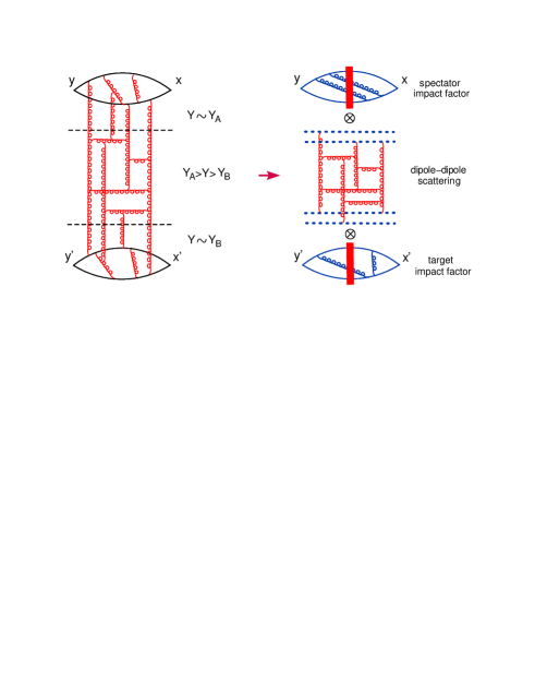
framework of the rapidity evolution of Wilson-line operators forming color dipoles mu94 ; nnn npb96 ; prld i ) the integral over the gluon (and gluino) fields with rapidity close to the rapidity of the spectator Y A subscript 𝑌 𝐴 Y_{A} ii ) the integral over the gluons with rapidity close to the rapidity of the target Y B subscript 𝑌 𝐵 Y_{B} iii ) the integral over the intermediate region of rapidities Y A > Y > Y B subscript 𝑌 𝐴 𝑌 subscript 𝑌 𝐵 Y_{A}>Y>Y_{B} Y A subscript 𝑌 𝐴 Y_{A} Y B subscript 𝑌 𝐵 Y_{B}
Figure 1: High-energy factorization
The high-energy (Regge) limit of a four-point amplitude A ( x , y ; x ′ , y ′ ) 𝐴 𝑥 𝑦 superscript 𝑥 ′ superscript 𝑦 ′ A(x,y;x^{\prime},y^{\prime})
x = ρ x ∗ p 1 + x ⟂ , y = ρ y ∗ p 2 + y ⟂ , formulae-sequence 𝑥 𝜌 subscript 𝑥 ∗ subscript 𝑝 1 subscript 𝑥 perpendicular-to 𝑦 𝜌 subscript 𝑦 ∗ subscript 𝑝 2 subscript 𝑦 perpendicular-to \displaystyle x=\rho x_{\ast}p_{1}+x_{\perp},~{}~{}~{}y=\rho y_{\ast}p_{2}+y_{\perp},~{}~{}~{}~{}~{}~{}~{}
x ′ = ρ ′ x ∙ p 2 + x ⟂ ′ , y ′ = ρ ′ y ∙ ′ p 2 + y ⟂ ′ formulae-sequence superscript 𝑥 ′ superscript 𝜌 ′ subscript 𝑥 ∙ subscript 𝑝 2 subscript superscript 𝑥 ′ perpendicular-to superscript 𝑦 ′ superscript 𝜌 ′ subscript superscript 𝑦 ′ ∙ subscript 𝑝 2 subscript superscript 𝑦 ′ perpendicular-to \displaystyle x^{\prime}=\rho^{\prime}x_{\bullet}p_{2}+x^{\prime}_{\perp},~{}~{}~{}y^{\prime}=\rho^{\prime}y^{\prime}_{\bullet}p_{2}+y^{\prime}_{\perp} (2)
with ρ , ρ ′ → ∞ → 𝜌 superscript 𝜌 ′
\rho,\rho^{\prime}\rightarrow\infty x ∗ > 0 > y ∗ subscript 𝑥 ∗ 0 subscript 𝑦 ∗ x_{\ast}>0>y_{\ast} x ∙ ′ > 0 > y ∙ ′ subscript superscript 𝑥 ′ ∙ 0 subscript superscript 𝑦 ′ ∙ x^{\prime}_{\bullet}>0>y^{\prime}_{\bullet} ρ → ∞ → 𝜌 \rho\rightarrow\infty ρ ′ → ∞ → superscript 𝜌 ′ \rho^{\prime}\rightarrow\infty x ∙ = p 1 μ x μ subscript 𝑥 ∙ superscript subscript 𝑝 1 𝜇 subscript 𝑥 𝜇 x_{\bullet}=p_{1}^{\mu}x_{\mu} x ∗ = p 2 μ x μ subscript 𝑥 ∗ superscript subscript 𝑝 2 𝜇 subscript 𝑥 𝜇 x_{\ast}=p_{2}^{\mu}x_{\mu} p 1 subscript 𝑝 1 p_{1} p 2 subscript 𝑝 2 p_{2} 2 ( p 1 , p 2 ) = s 2 subscript 𝑝 1 subscript 𝑝 2 𝑠 2(p_{1},p_{2})=s x ± = 1 2 ( x 0 ± x 3 ) superscript 𝑥 plus-or-minus 1 2 plus-or-minus superscript 𝑥 0 superscript 𝑥 3 x^{\pm}={1\over\sqrt{2}}(x^{0}\pm x^{3}) x ∗ = x + s / 2 , x ∙ = x − s / 2 formulae-sequence subscript 𝑥 ∗ superscript 𝑥 𝑠 2 subscript 𝑥 ∙ superscript 𝑥 𝑠 2 x_{\ast}=x^{+}\sqrt{s/2},~{}x_{\bullet}=x^{-}\sqrt{s/2} x = 2 s x ∗ p 1 + 2 s x ∙ p 2 + x ⟂ 𝑥 2 𝑠 subscript 𝑥 ∗ subscript 𝑝 1 2 𝑠 subscript 𝑥 ∙ subscript 𝑝 2 subscript 𝑥 perpendicular-to x={2\over s}x_{\ast}p_{1}+{2\over s}x_{\bullet}p_{2}+x_{\perp} x 2 = 4 s x ∙ x ∗ − x → ⟂ 2 superscript 𝑥 2 4 𝑠 subscript 𝑥 ∙ subscript 𝑥 ∗ superscript subscript → 𝑥 perpendicular-to 2 x^{2}={4\over s}x_{\bullet}x_{\ast}-\vec{x}_{\perp}^{2} 2 ( 0 , 0 , z ⟂ ) 0 0 subscript 𝑧 perpendicular-to (0,0,z_{\perp})
For simplicity, let us consider correlation function of four scalar currents
( x − y ) 4 ( x ′ − y ′ ) 4 ⟨ 𝒪 ( x ) 𝒪 † ( y ) 𝒪 ( x ′ ) 𝒪 † ( y ′ ) ⟩ superscript 𝑥 𝑦 4 superscript superscript 𝑥 ′ superscript 𝑦 ′ 4 delimited-⟨⟩ 𝒪 𝑥 superscript 𝒪 † 𝑦 𝒪 superscript 𝑥 ′ superscript 𝒪 † superscript 𝑦 ′ \displaystyle(x-y)^{4}(x^{\prime}-y^{\prime})^{4}\langle{\cal O}(x){\cal O}^{\dagger}(y){\cal O}(x^{\prime}){\cal O}^{\dagger}(y^{\prime})\rangle~{} (3)
where 𝒪 ≡ 4 π 2 2 N c 2 − 1 Tr { Z 2 } 𝒪 4 superscript 𝜋 2 2 superscript subscript 𝑁 𝑐 2 1 Tr superscript Z 2 {{\cal O}}\equiv{4\pi^{2}\sqrt{2}\over\sqrt{N_{c}^{2}-1}}{\rm Tr\{Z^{2}\}} Z = 1 2 ( ϕ 1 + i ϕ 2 ) 𝑍 1 2 subscript italic-ϕ 1 𝑖 subscript italic-ϕ 2 Z={1\over\sqrt{2}}(\phi_{1}+i\phi_{2})
In a conformal theory this four-point amplitude A ( x , y ; x ′ , y ′ ) 𝐴 𝑥 𝑦 superscript 𝑥 ′ superscript 𝑦 ′ A(x,y;x^{\prime},y^{\prime})
R = ( x − x ′ ) 2 ( y − y ′ ) 2 ( x − y ) 2 ( x ′ − y ′ ) 2 , 𝑅 superscript 𝑥 superscript 𝑥 ′ 2 superscript 𝑦 superscript 𝑦 ′ 2 superscript 𝑥 𝑦 2 superscript superscript 𝑥 ′ superscript 𝑦 ′ 2 \displaystyle R~{}=~{}{(x-x^{\prime})^{2}(y-y^{\prime})^{2}\over(x-y)^{2}(x^{\prime}-y^{\prime})^{2}},~{}~{}~{}~{}
r = R [ 1 − ( x − y ′ ) 2 ( y − x ′ ) 2 ( x − x ′ ) 2 ( y − y ′ ) 2 + 1 R ] 2 𝑟 𝑅 superscript delimited-[] 1 superscript 𝑥 superscript 𝑦 ′ 2 superscript 𝑦 superscript 𝑥 ′ 2 superscript 𝑥 superscript 𝑥 ′ 2 superscript 𝑦 superscript 𝑦 ′ 2 1 𝑅 2 \displaystyle r~{}=~{}R\Big{[}1-{(x-y^{\prime})^{2}(y-x^{\prime})^{2}\over(x-x^{\prime})^{2}(y-y^{\prime})^{2}}+{1\over R}\Big{]}^{2} (4)
In the Regge limit (2 R 𝑅 R ρ 2 ρ ′ 2 superscript 𝜌 2 superscript superscript 𝜌 ′ 2 \rho^{2}{\rho^{\prime}}^{2} r 𝑟 r ρ 𝜌 \rho ρ ′ superscript 𝜌 ′ \rho^{\prime}
As demonstrated in Ref. cornalba ν 𝜈 \nu
( x − y ) 4 ( x ′ − y ′ ) 4 ⟨ 𝒪 ( x ) 𝒪 † ( y ) 𝒪 ( x ′ ) 𝒪 † ( y ′ ) ⟩ superscript 𝑥 𝑦 4 superscript superscript 𝑥 ′ superscript 𝑦 ′ 4 delimited-⟨⟩ 𝒪 𝑥 superscript 𝒪 † 𝑦 𝒪 superscript 𝑥 ′ superscript 𝒪 † superscript 𝑦 ′ \displaystyle(x-y)^{4}(x^{\prime}-y^{\prime})^{4}\langle{\cal O}(x){\cal O}^{\dagger}(y){\cal O}(x^{\prime}){\cal O}^{\dagger}(y^{\prime})\rangle~{} (5)
= i 2 ∫ 𝑑 ν f ~ + ( ν ) tanh π ν ν F ( ν ) Ω ( r , ν ) R 1 2 ω ( ν ) absent 𝑖 2 differential-d 𝜈 subscript ~ 𝑓 𝜈 𝜋 𝜈 𝜈 𝐹 𝜈 Ω 𝑟 𝜈 superscript 𝑅 1 2 𝜔 𝜈 \displaystyle=~{}{i\over 2}\!\int\!d\nu~{}\tilde{f}_{+}(\nu){\tanh\pi\nu\over\nu}F(\nu)\Omega(r,\nu)R^{{1\over 2}\omega(\nu)}
Here ω ( ν ) ≡ ω ( 0 , ν ) 𝜔 𝜈 𝜔 0 𝜈 \omega(\nu)\equiv\omega(0,\nu) f ~ + ( ν ) ≡ f ~ + ( ω ( ν ) ) subscript ~ 𝑓 𝜈 subscript ~ 𝑓 𝜔 𝜈 \tilde{f}_{+}(\nu)\equiv\tilde{f}_{+}(\omega(\nu)) f ~ + ( ω ) = ( e i π ω − 1 ) / sin π ω subscript ~ 𝑓 𝜔 superscript 𝑒 𝑖 𝜋 𝜔 1 𝜋 𝜔 \tilde{f}_{+}(\omega)=(e^{i\pi\omega}-1)/\sin\pi\omega F ( ν ) 𝐹 𝜈 F(\nu) Ω ( r , ν ) Ω 𝑟 𝜈 \Omega(r,\nu) penecostalba
Ω ( r , ν ) = ν 2 π 3 ∫ d 2 z [ κ 2 ( 2 κ ⋅ ζ ) 2 ] 1 2 + i ν [ κ ′ 2 ( 2 κ ′ ⋅ ζ ) 2 ] 1 2 − i ν Ω 𝑟 𝜈 superscript 𝜈 2 superscript 𝜋 3 superscript 𝑑 2 𝑧 superscript delimited-[] superscript 𝜅 2 superscript ⋅ 2 𝜅 𝜁 2 1 2 𝑖 𝜈 superscript delimited-[] superscript superscript 𝜅 ′ 2 superscript ⋅ 2 superscript 𝜅 ′ 𝜁 2 1 2 𝑖 𝜈 \displaystyle\Omega(r,\nu)~{}=~{}{\nu^{2}\over\pi^{3}}\!\int\!d^{2}z\Big{[}{\kappa^{2}\over(2\kappa\cdot\zeta)^{2}}\Big{]}^{{1\over 2}+i\nu}\Big{[}{{\kappa^{\prime}}^{2}\over(2\kappa^{\prime}\cdot\zeta)^{2}}\Big{]}^{{1\over 2}-i\nu} (6)
where ζ ≡ p 1 + z ⟂ 2 s p 2 + z ⟂ 𝜁 subscript 𝑝 1 superscript subscript 𝑧 perpendicular-to 2 𝑠 subscript 𝑝 2 subscript 𝑧 perpendicular-to \zeta\equiv p_{1}+{z_{\perp}^{2}\over s}p_{2}+z_{\perp}
κ = s 2 x ∗ ( p 1 − x 2 s p 2 + x ⟂ ) − s 2 y ∗ ( p 1 − y 2 s p 2 + y ⟂ ) 𝜅 𝑠 2 subscript 𝑥 ∗ subscript 𝑝 1 superscript 𝑥 2 𝑠 subscript 𝑝 2 subscript 𝑥 perpendicular-to 𝑠 2 subscript 𝑦 ∗ subscript 𝑝 1 superscript 𝑦 2 𝑠 subscript 𝑝 2 subscript 𝑦 perpendicular-to \displaystyle\kappa~{}=~{}{\sqrt{s}\over 2x_{\ast}}(p_{1}-{x^{2}\over s}p_{2}+x_{\perp})-{\sqrt{s}\over 2y_{\ast}}(p_{1}-{y^{2}\over s}p_{2}+y_{\perp}) (7)
κ ′ = s 2 x ∙ ′ ( p 1 − x ′ 2 s p 2 + x ⟂ ′ ) − s 2 y ∙ ′ ( p 1 − y ′ 2 s p 2 + y ⟂ ′ ) superscript 𝜅 ′ 𝑠 2 subscript superscript 𝑥 ′ ∙ subscript 𝑝 1 superscript superscript 𝑥 ′ 2 𝑠 subscript 𝑝 2 subscript superscript 𝑥 ′ perpendicular-to 𝑠 2 subscript superscript 𝑦 ′ ∙ subscript 𝑝 1 superscript superscript 𝑦 ′ 2 𝑠 subscript 𝑝 2 subscript superscript 𝑦 ′ perpendicular-to \displaystyle\kappa^{\prime}~{}=~{}{\sqrt{s}\over 2x^{\prime}_{\bullet}}(p_{1}-{{x^{\prime}}^{2}\over s}p_{2}+x^{\prime}_{\perp})-{\sqrt{s}\over 2y^{\prime}_{\bullet}}(p_{1}-{{y^{\prime}}^{2}\over s}p_{2}+y^{\prime}_{\perp})
are two SL(2,C)-invariant vectors penecostalba
κ 2 κ ′ 2 = 1 R and 4 ( κ ⋅ κ ′ ) 2 = r R formulae-sequence superscript 𝜅 2 superscript superscript 𝜅 ′ 2 1 𝑅 and
4 superscript ⋅ 𝜅 superscript 𝜅 ′ 2 𝑟 𝑅 \kappa^{2}{\kappa^{\prime}}^{2}~{}=~{}{1\over R}~{}~{}~{}~{}~{}~{}{\rm and}~{}~{}~{}~{}~{}~{}~{}~{}4(\kappa\cdot\kappa^{\prime})^{2}~{}=~{}{r\over R} (8)
Here x 2 = − x ⟂ 2 , x ′ 2 = − x ′ ⟂ 2 formulae-sequence superscript 𝑥 2 superscript subscript 𝑥 perpendicular-to 2 superscript superscript 𝑥 ′ 2 superscript subscript superscript 𝑥 ′ perpendicular-to 2 x^{2}=-x_{\perp}^{2},~{}{x^{\prime}}^{2}=-{x^{\prime}}_{\perp}^{2} y 𝑦 y ≡ \equiv ρ , ρ ′ 𝜌 superscript 𝜌 ′
\rho,\rho^{\prime} R 1 2 ω ( ν ) superscript 𝑅 1 2 𝜔 𝜈 R^{{1\over 2}\omega(\nu)}
The dynamical information about the conformal theory is encoded in two functions: pomeron intercept and pomeron residue.
The pomeron intercept is known both in the small and large α s subscript 𝛼 𝑠 \alpha_{s} α s subscript 𝛼 𝑠 \alpha_{s} bfkl
ω ( ν ) = α s π N c [ χ ( ν ) + α s N c 4 π δ ( ν ) ] , 𝜔 𝜈 subscript 𝛼 𝑠 𝜋 subscript 𝑁 𝑐 delimited-[] 𝜒 𝜈 subscript 𝛼 𝑠 subscript 𝑁 𝑐 4 𝜋 𝛿 𝜈 \displaystyle\omega(\nu)~{}=~{}{\alpha_{s}\over\pi}N_{c}\Big{[}\chi(\nu)+{\alpha_{s}N_{c}\over 4\pi}\delta(\nu)\Big{]},
δ ( ν ) = 6 ζ ( 3 ) − π 2 3 χ ( ν ) + χ ′′ ( ν ) − 2 Φ ( ν ) − 2 Φ ( − ν ) 𝛿 𝜈 6 𝜁 3 superscript 𝜋 2 3 𝜒 𝜈 superscript 𝜒 ′′ 𝜈 2 Φ 𝜈 2 Φ 𝜈 \displaystyle\delta(\nu)~{}=~{}6\zeta(3)-{\pi^{2}\over 3}\chi(\nu)+\chi^{\prime\prime}(\nu)-~{}2\Phi(\nu)-2\Phi(-\nu) (9)
where χ ( ν ) = 2 ψ ( 1 ) − ψ ( 1 2 + i ν ) − ψ ( 1 2 − i ν ) 𝜒 𝜈 2 𝜓 1 𝜓 1 2 𝑖 𝜈 𝜓 1 2 𝑖 𝜈 \chi(\nu)=2\psi(1)-\psi({1\over 2}+i\nu)-\psi({1\over 2}-i\nu) lipkot
Φ ( ν ) = − ∫ 0 1 d t 1 + t t − 1 2 + i ν [ π 2 6 + 2 L i 2 ( t ) ] Φ 𝜈 superscript subscript 0 1 𝑑 𝑡 1 𝑡 superscript 𝑡 1 2 𝑖 𝜈 delimited-[] superscript 𝜋 2 6 2 L subscript i 2 𝑡 \displaystyle\Phi(\nu)~{}=~{}-\int_{0}^{1}\!{dt\over 1+t}~{}t^{-{1\over 2}+i\nu}\Big{[}{\pi^{2}\over 6}+2{\rm Li}_{2}(t)\Big{]} (10)
Our main goal is the description of the amplitude in the next-to-leading order in perturbation theory, but
it is worth noting that the pomeron intercept is known also in the limit of large
’t Hooft coupling λ = 4 π α s N c 𝜆 4 𝜋 subscript 𝛼 𝑠 subscript 𝑁 𝑐 \lambda=4\pi\alpha_{s}N_{c}
ω ( ν ) = 2 − ν 2 + 4 2 λ 𝜔 𝜈 2 superscript 𝜈 2 4 2 𝜆 \omega(\nu)~{}=~{}2-{\nu^{2}+4\over 2\sqrt{\lambda}} (11)
where 2 is the graviton spin and the first correction was calculated in Ref. klov ; brtan
The pomeron residue F ( ν ) 𝐹 𝜈 F(\nu) penecostalba ; penecostalba2 ; penedones cornalba
F ( ν ) → λ → 0 λ 2 π sin π ν 4 ν cos 3 π ν , F ( ν ) → λ → ∞ π 3 ν 2 ( 1 + ν ) 2 sinh 2 π ν formulae-sequence superscript → → 𝜆 0 𝐹 𝜈 superscript 𝜆 2 𝜋 𝜋 𝜈 4 𝜈 superscript 3 𝜋 𝜈 superscript → → 𝜆 𝐹 𝜈 superscript 𝜋 3 superscript 𝜈 2 superscript 1 𝜈 2 superscript 2 𝜋 𝜈 F(\nu)~{}\stackrel{{\scriptstyle\lambda\rightarrow 0}}{{\rightarrow}}~{}\lambda^{2}{\pi\sin\pi\nu\over 4\nu\cos^{3}\pi\nu},~{}~{}~{}~{}F(\nu)~{}\stackrel{{\scriptstyle\lambda\rightarrow\infty}}{{\rightarrow}}~{}{\pi^{3}\nu^{2}(1+\nu)^{2}\over\sinh^{2}\pi\nu} (12)
To find the NLO amplitude, we must also calculate the “pomeron residue” F ( ν ) 𝐹 𝜈 F(\nu) npb96
II Operator expansion in conformal dipoles
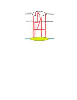
As we discussed above, the main idea behind the high-energy operator expansion is the rapidity factorization. At the first step, we integrate
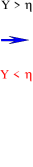
over gluons with rapidities Y > η 𝑌 𝜂 Y>\eta Y < η 𝑌 𝜂 Y<\eta
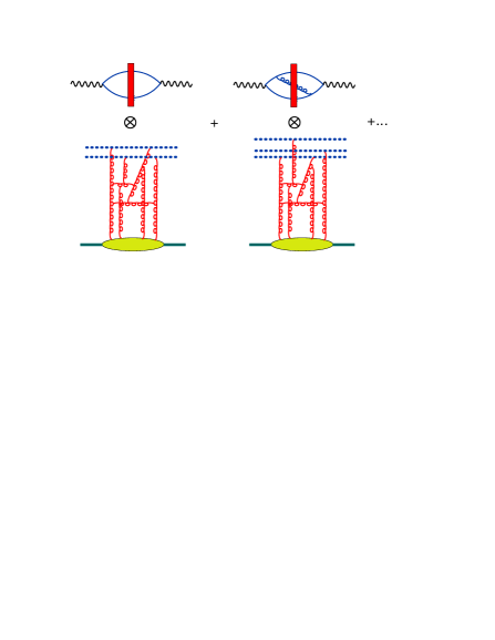
Figure 2: High-energy operator expansion in Wilson lines
The result of the integration is the coefficient
function (“impact factor”) in front of the Wilson-line operators with rapidities up to η = ln σ 𝜂 𝜎 \eta=\ln\sigma
U x σ = Pexp [ i g ∫ − ∞ ∞ 𝑑 u p 1 μ A μ σ ( u p 1 + x ⟂ ) ] subscript superscript 𝑈 𝜎 𝑥 Pexp delimited-[] 𝑖 𝑔 superscript subscript differential-d 𝑢 superscript subscript 𝑝 1 𝜇 subscript superscript 𝐴 𝜎 𝜇 𝑢 subscript 𝑝 1 subscript 𝑥 perpendicular-to \displaystyle U^{\sigma}_{x}~{}=~{}{\rm Pexp}\Big{[}ig\!\int_{-\infty}^{\infty}\!\!du~{}p_{1}^{\mu}A^{\sigma}_{\mu}(up_{1}+x_{\perp})\Big{]}
A μ σ ( x ) = ∫ d 4 k θ ( σ − | α k | ) e − i k ⋅ x A μ ( k ) subscript superscript 𝐴 𝜎 𝜇 𝑥 superscript 𝑑 4 𝑘 𝜃 𝜎 subscript 𝛼 𝑘 superscript 𝑒 ⋅ 𝑖 𝑘 𝑥 subscript 𝐴 𝜇 𝑘 \displaystyle A^{\sigma}_{\mu}(x)~{}=~{}\int\!d^{4}k~{}\theta(\sigma-|\alpha_{k}|)e^{-ik\cdot x}A_{\mu}(k) (13)
For the T 𝑇 T 𝒪 𝒪 {\cal O} nlobksym
( x − y ) 4 T { 𝒪 ^ ( x ) 𝒪 ^ † ( y ) } = 1 π 2 ( N c 2 − 1 ) ∫ d 2 z 1 d 2 z 2 z 12 4 ℛ 2 [ Tr { U ^ z 1 σ U ^ z 2 † σ } \displaystyle(x-y)^{4}T\{\hat{\cal O}(x)\hat{\cal O}^{\dagger}(y)\}~{}=~{}{1\over\pi^{2}(N_{c}^{2}-1)}\!\int\!{d^{2}z_{1}d^{2}z_{2}\over z_{12}^{4}}~{}{\cal R}^{2}~{}\Big{[}{\rm Tr}\{\hat{U}^{\sigma}_{z_{1}}\hat{U}^{\dagger\sigma}_{z_{2}}\} (14)
− α s π 2 ∫ d 2 z 3 z 12 2 z 13 2 z 23 2 [ ln s 4 σ 𝒵 3 − i π 2 + C ] [ Tr { T n U ^ z 1 σ U ^ z 3 † σ T n U ^ z 3 σ U ^ z 2 † σ } − N c Tr { U ^ z 1 σ U ^ z 2 † σ } ] subscript 𝛼 𝑠 superscript 𝜋 2 superscript 𝑑 2 subscript 𝑧 3 superscript subscript 𝑧 12 2 superscript subscript 𝑧 13 2 superscript subscript 𝑧 23 2 delimited-[] 𝑠 4 𝜎 subscript 𝒵 3 𝑖 𝜋 2 𝐶 delimited-[] Tr superscript 𝑇 𝑛 subscript superscript ^ 𝑈 𝜎 subscript 𝑧 1 subscript superscript ^ 𝑈 † absent 𝜎 subscript 𝑧 3 superscript 𝑇 𝑛 subscript superscript ^ 𝑈 𝜎 subscript 𝑧 3 subscript superscript ^ 𝑈 † absent 𝜎 subscript 𝑧 2 subscript 𝑁 𝑐 Tr subscript superscript ^ 𝑈 𝜎 subscript 𝑧 1 subscript superscript ^ 𝑈 † absent 𝜎 subscript 𝑧 2 \displaystyle-~{}{\alpha_{s}\over\pi^{2}}\!\int\!d^{2}z_{3}~{}{z_{12}^{2}\over z_{13}^{2}z_{23}^{2}}\Big{[}\ln{s\over 4}\sigma{\cal Z}_{3}-{i\pi\over 2}+C\Big{]}[{\rm Tr}\{T^{n}\hat{U}^{\sigma}_{z_{1}}\hat{U}^{\dagger\sigma}_{z_{3}}T^{n}\hat{U}^{\sigma}_{z_{3}}\hat{U}^{\dagger\sigma}_{z_{2}}\}-N_{c}{\rm Tr}\{\hat{U}^{\sigma}_{z_{1}}\hat{U}^{\dagger\sigma}_{z_{2}}\}]
Hereafter we use the notations 𝒵 i ≡ ( x − z i ) 2 x ∗ − ( y − z i ) 2 y ∗ subscript 𝒵 𝑖 superscript 𝑥 subscript 𝑧 𝑖 2 subscript 𝑥 ∗ superscript 𝑦 subscript 𝑧 𝑖 2 subscript 𝑦 ∗ {\cal Z}_{i}\equiv{(x-z_{i})^{2}\over x_{\ast}}-{(y-z_{i})^{2}\over y_{\ast}}
ℛ = ( x − y ) 2 z 12 2 x ∗ y ∗ 𝒵 1 𝒵 2 = κ 2 ( ζ 1 ⋅ ζ 2 ) 2 ( κ ⋅ ζ 1 ) ( κ ⋅ ζ 2 ) ℛ superscript 𝑥 𝑦 2 superscript subscript 𝑧 12 2 subscript 𝑥 ∗ subscript 𝑦 ∗ subscript 𝒵 1 subscript 𝒵 2 superscript 𝜅 2 ⋅ subscript 𝜁 1 subscript 𝜁 2 2 ⋅ 𝜅 subscript 𝜁 1 ⋅ 𝜅 subscript 𝜁 2 {\cal R}~{}=~{}{(x-y)^{2}z_{12}^{2}\over x_{\ast}y_{\ast}{\cal Z}_{1}{\cal Z}_{2}}~{}=~{}{\kappa^{2}(\zeta_{1}\cdot\zeta_{2})\over 2(\kappa\cdot\zeta_{1})(\kappa\cdot\zeta_{2})} (15)
Note that the l.h.s. of the Eq. (14 13 p 1 subscript 𝑝 1 p_{1} α 𝛼 \alpha 𝒩 = 4 𝒩 4 {\cal N}=4 nlobksym
[ Tr { U ^ z 1 U ^ z 2 † } ] a , Y conf superscript subscript delimited-[] Tr subscript ^ 𝑈 subscript 𝑧 1 subscript superscript ^ 𝑈 † subscript 𝑧 2 𝑎 𝑌
conf \displaystyle[{\rm Tr}\{\hat{U}_{z_{1}}\hat{U}^{\dagger}_{z_{2}}\}\big{]}_{a,Y}^{\rm conf}~{} (16)
= Tr { U ^ z 1 σ U ^ z 2 † σ } + α s 2 π 2 ∫ d 2 z 3 z 12 2 z 13 2 z 23 2 [ Tr { T n U ^ z 1 σ U ^ z 3 † σ T n U ^ z 3 σ U ^ z 2 † σ } − N c Tr { U ^ z 1 σ U ^ z 2 † σ } ] ln 4 a z 12 2 s z 13 2 z 23 2 + O ( α s 2 ) absent Tr subscript superscript ^ 𝑈 𝜎 subscript 𝑧 1 subscript superscript ^ 𝑈 † absent 𝜎 subscript 𝑧 2 subscript 𝛼 𝑠 2 superscript 𝜋 2 superscript 𝑑 2 subscript 𝑧 3 superscript subscript 𝑧 12 2 superscript subscript 𝑧 13 2 superscript subscript 𝑧 23 2 delimited-[] Tr superscript 𝑇 𝑛 subscript superscript ^ 𝑈 𝜎 subscript 𝑧 1 subscript superscript ^ 𝑈 † absent 𝜎 subscript 𝑧 3 superscript 𝑇 𝑛 subscript superscript ^ 𝑈 𝜎 subscript 𝑧 3 subscript superscript ^ 𝑈 † absent 𝜎 subscript 𝑧 2 subscript 𝑁 𝑐 Tr subscript superscript ^ 𝑈 𝜎 subscript 𝑧 1 subscript superscript ^ 𝑈 † absent 𝜎 subscript 𝑧 2 4 𝑎 superscript subscript 𝑧 12 2 𝑠 superscript subscript 𝑧 13 2 superscript subscript 𝑧 23 2 𝑂 superscript subscript 𝛼 𝑠 2 \displaystyle=~{}{\rm Tr}\{\hat{U}^{\sigma}_{z_{1}}\hat{U}^{\dagger\sigma}_{z_{2}}\}+{\alpha_{s}\over 2\pi^{2}}\!\int\!d^{2}z_{3}~{}{z_{12}^{2}\over z_{13}^{2}z_{23}^{2}}[{\rm Tr}\{T^{n}\hat{U}^{\sigma}_{z_{1}}\hat{U}^{\dagger\sigma}_{z_{3}}T^{n}\hat{U}^{\sigma}_{z_{3}}\hat{U}^{\dagger\sigma}_{z_{2}}\}-N_{c}{\rm Tr}\{\hat{U}^{\sigma}_{z_{1}}\hat{U}^{\dagger\sigma}_{z_{2}}\}]\ln{4az_{12}^{2}\over sz_{13}^{2}z_{23}^{2}}~{}+~{}O(\alpha_{s}^{2})
where a 𝑎 a a → a e − 2 η → 𝑎 𝑎 superscript 𝑒 2 𝜂 a\rightarrow ae^{-2\eta} [ Tr { U ^ z 1 σ U ^ z 2 † σ } ] a conf superscript subscript delimited-[] Tr subscript superscript ^ 𝑈 𝜎 subscript 𝑧 1 subscript superscript ^ 𝑈 † absent 𝜎 subscript 𝑧 2 𝑎 conf [{\rm Tr}\{\hat{U}^{\sigma}_{z_{1}}\hat{U}^{\dagger\sigma}_{z_{2}}\}\big{]}_{a}^{\rm conf} η = ln σ 𝜂 𝜎 \eta=\ln\sigma a 𝑎 a
[ Tr { U ^ z 1 U ^ z 2 † } ] a conf superscript subscript delimited-[] Tr subscript ^ 𝑈 subscript 𝑧 1 subscript superscript ^ 𝑈 † subscript 𝑧 2 𝑎 conf \displaystyle[{\rm Tr}\{\hat{U}_{z_{1}}\hat{U}^{\dagger}_{z_{2}}\}\big{]}_{a}^{\rm conf}~{} (17)
= Tr { U ^ z 1 σ U ^ z 2 † σ } + α s 2 π 2 ∫ d 2 z 3 z 12 2 z 13 2 z 23 2 [ Tr { T n U ^ z 1 σ U ^ z 3 † σ T n U ^ z 3 σ U ^ z 2 † σ } − N c Tr { U ^ z 1 σ U ^ z 2 † σ } ] ln 4 a z 12 2 σ 2 s z 13 2 z 23 2 + O ( α s 2 ) absent Tr subscript superscript ^ 𝑈 𝜎 subscript 𝑧 1 subscript superscript ^ 𝑈 † absent 𝜎 subscript 𝑧 2 subscript 𝛼 𝑠 2 superscript 𝜋 2 superscript 𝑑 2 subscript 𝑧 3 superscript subscript 𝑧 12 2 superscript subscript 𝑧 13 2 superscript subscript 𝑧 23 2 delimited-[] Tr superscript 𝑇 𝑛 subscript superscript ^ 𝑈 𝜎 subscript 𝑧 1 subscript superscript ^ 𝑈 † absent 𝜎 subscript 𝑧 3 superscript 𝑇 𝑛 subscript superscript ^ 𝑈 𝜎 subscript 𝑧 3 subscript superscript ^ 𝑈 † absent 𝜎 subscript 𝑧 2 subscript 𝑁 𝑐 Tr subscript superscript ^ 𝑈 𝜎 subscript 𝑧 1 subscript superscript ^ 𝑈 † absent 𝜎 subscript 𝑧 2 4 𝑎 superscript subscript 𝑧 12 2 superscript 𝜎 2 𝑠 superscript subscript 𝑧 13 2 superscript subscript 𝑧 23 2 𝑂 superscript subscript 𝛼 𝑠 2 \displaystyle=~{}{\rm Tr}\{\hat{U}^{\sigma}_{z_{1}}\hat{U}^{\dagger\sigma}_{z_{2}}\}+~{}{\alpha_{s}\over 2\pi^{2}}\!\int\!d^{2}z_{3}~{}{z_{12}^{2}\over z_{13}^{2}z_{23}^{2}}[{\rm Tr}\{T^{n}\hat{U}^{\sigma}_{z_{1}}\hat{U}^{\dagger\sigma}_{z_{3}}T^{n}\hat{U}^{\sigma}_{z_{3}}\hat{U}^{\dagger\sigma}_{z_{2}}\}-N_{c}{\rm Tr}\{\hat{U}^{\sigma}_{z_{1}}\hat{U}^{\dagger\sigma}_{z_{2}}\}]\ln{4az_{12}^{2}\over\sigma^{2}sz_{13}^{2}z_{23}^{2}}~{}+~{}O(\alpha_{s}^{2})
Using the leading-order evolution equation npb96
d d η Tr { U ^ z 1 σ U ^ z 2 † σ } = σ d d σ Tr { U ^ z 1 σ U ^ z 2 † σ } = α s π 2 ∫ d 2 z 3 z 12 2 z 13 2 z 23 2 [ Tr { T n U ^ z 1 σ U ^ z 3 † σ T n U ^ z 3 σ U ^ z 2 † σ } − N c Tr { U ^ z 1 σ U ^ z 2 † σ } ] 𝑑 𝑑 𝜂 Tr superscript subscript ^ 𝑈 subscript 𝑧 1 𝜎 subscript superscript ^ 𝑈 † absent 𝜎 subscript 𝑧 2 𝜎 𝑑 𝑑 𝜎 Tr superscript subscript ^ 𝑈 subscript 𝑧 1 𝜎 subscript superscript ^ 𝑈 † absent 𝜎 subscript 𝑧 2 subscript 𝛼 𝑠 superscript 𝜋 2 superscript 𝑑 2 subscript 𝑧 3 superscript subscript 𝑧 12 2 superscript subscript 𝑧 13 2 superscript subscript 𝑧 23 2 delimited-[] Tr superscript 𝑇 𝑛 subscript superscript ^ 𝑈 𝜎 subscript 𝑧 1 subscript superscript ^ 𝑈 † absent 𝜎 subscript 𝑧 3 superscript 𝑇 𝑛 subscript superscript ^ 𝑈 𝜎 subscript 𝑧 3 subscript superscript ^ 𝑈 † absent 𝜎 subscript 𝑧 2 subscript 𝑁 𝑐 Tr subscript superscript ^ 𝑈 𝜎 subscript 𝑧 1 subscript superscript ^ 𝑈 † absent 𝜎 subscript 𝑧 2 {d\over d\eta}{\rm Tr}\{\hat{U}_{z_{1}}^{\sigma}\hat{U}^{\dagger\sigma}_{z_{2}}\}~{}=~{}\sigma{d\over d\sigma}{\rm Tr}\{\hat{U}_{z_{1}}^{\sigma}\hat{U}^{\dagger\sigma}_{z_{2}}\}~{}=~{}{\alpha_{s}\over\pi^{2}}\!\int\!d^{2}z_{3}~{}{z_{12}^{2}\over z_{13}^{2}z_{23}^{2}}[{\rm Tr}\{T^{n}\hat{U}^{\sigma}_{z_{1}}\hat{U}^{\dagger\sigma}_{z_{3}}T^{n}\hat{U}^{\sigma}_{z_{3}}\hat{U}^{\dagger\sigma}_{z_{2}}\}-N_{c}{\rm Tr}\{\hat{U}^{\sigma}_{z_{1}}\hat{U}^{\dagger\sigma}_{z_{2}}\}] (18)
it is easy to see that d d η [ Tr { U ^ z 1 U ^ z 2 † } ] a conf = 0 𝑑 𝑑 𝜂 superscript subscript delimited-[] Tr subscript ^ 𝑈 subscript 𝑧 1 subscript superscript ^ 𝑈 † subscript 𝑧 2 𝑎 conf 0 {d\over d\eta}[{\rm Tr}\{\hat{U}_{z_{1}}\hat{U}^{\dagger}_{z_{2}}\}\big{]}_{a}^{\rm conf}~{}=~{}0 O ( α s 2 ) 𝑂 superscript subscript 𝛼 𝑠 2 O(\alpha_{s}^{2})
Rewritten in terms of conformal dipoles (17 14
( x − y ) 4 T { 𝒪 ^ ( x ) 𝒪 ^ † ( y ) } = 1 π 2 ( N c 2 − 1 ) ∫ d 2 z 1 d 2 z 2 z 12 4 ℛ 2 { [ Tr { U ^ z 1 U ^ z 2 † } ] a conf \displaystyle(x-y)^{4}T\{\hat{\cal O}(x)\hat{\cal O}^{\dagger}(y)\}~{}=~{}{1\over\pi^{2}(N_{c}^{2}-1)}\!\int\!{d^{2}z_{1}d^{2}z_{2}\over z_{12}^{4}}~{}{\cal R}^{2}~{}\Big{\{}[{\rm Tr}\{\hat{U}_{z_{1}}\hat{U}^{\dagger}_{z_{2}}\}]_{a}^{\rm conf}
− α s 2 π 2 ∫ d 2 z 3 z 12 2 z 13 2 z 23 2 ( ln a s z 12 2 4 z 13 2 z 23 2 𝒵 3 2 − i π + 2 C ) [ Tr { T n U ^ z 1 U ^ z 3 † T n U ^ z 3 U ^ z 2 † } − N c Tr { U ^ z 1 U ^ z 2 † } ] a } \displaystyle-~{}{\alpha_{s}\over 2\pi^{2}}\!\int\!d^{2}z_{3}{z_{12}^{2}\over z_{13}^{2}z_{23}^{2}}\Big{(}\ln{asz_{12}^{2}\over 4z_{13}^{2}z_{23}^{2}}{\cal Z}_{3}^{2}-i\pi+2C\Big{)}[{\rm Tr}\{T^{n}\hat{U}_{z_{1}}\hat{U}^{\dagger}_{z_{3}}T^{n}\hat{U}_{z_{3}}\hat{U}^{\dagger}_{z_{2}}\}-N_{c}{\rm Tr}\{\hat{U}_{z_{1}}\hat{U}^{\dagger}_{z_{2}}\}]_{a}\Big{\}} (19)
We need to choose the new “rapidity cutoff” a 𝑎 a ≡ \equiv ρ 𝜌 \rho ρ → ∞ → 𝜌 \rho\rightarrow\infty a 𝑎 a a 0 = − κ − 2 + i ϵ = − 4 x ∗ y ∗ s ( x − y ) 2 + i ϵ subscript 𝑎 0 superscript 𝜅 2 𝑖 italic-ϵ 4 subscript 𝑥 ∗ subscript 𝑦 ∗ 𝑠 superscript 𝑥 𝑦 2 𝑖 italic-ϵ a_{0}=-\kappa^{-2}+i\epsilon=-{4x_{\ast}y_{\ast}\over s(x-y)^{2}}+i\epsilon
( x − y ) 4 T { 𝒪 ^ ( x ) 𝒪 ^ † ( y ) } = 1 π 2 ( N c 2 − 1 ) ∫ d 2 z 1 d 2 z 2 z 12 4 ℛ 2 { [ Tr { U ^ z 1 σ U ^ z 2 † σ } ] a 0 conf \displaystyle(x-y)^{4}T\{\hat{\cal O}(x)\hat{\cal O}^{\dagger}(y)\}~{}=~{}{1\over\pi^{2}(N_{c}^{2}-1)}\!\int\!{d^{2}z_{1}d^{2}z_{2}\over z_{12}^{4}}~{}{\cal R}^{2}~{}\Big{\{}[{\rm Tr}\{\hat{U}^{\sigma}_{z_{1}}\hat{U}^{\dagger\sigma}_{z_{2}}\}]_{a_{0}}^{\rm conf}
− α s 2 π 2 ∫ d 2 z 3 z 12 2 z 13 2 z 23 2 [ ln x ∗ y ∗ z 12 2 ( x − y ) 2 z 13 2 z 23 2 𝒵 3 2 + 2 C ] [ Tr { T n U ^ z 1 σ U ^ z 3 † σ T n U ^ z 3 σ U ^ z 2 † σ } − N c Tr { U ^ z 1 σ U ^ z 2 † σ } ] } \displaystyle-~{}{\alpha_{s}\over 2\pi^{2}}\!\int\!d^{2}z_{3}{z_{12}^{2}\over z_{13}^{2}z_{23}^{2}}\Big{[}\ln{x_{\ast}y_{\ast}z_{12}^{2}\over(x-y)^{2}z_{13}^{2}z_{23}^{2}}{\cal Z}_{3}^{2}+2C\Big{]}[{\rm Tr}\{T^{n}\hat{U}^{\sigma}_{z_{1}}\hat{U}^{\dagger\sigma}_{z_{3}}T^{n}\hat{U}^{\sigma}_{z_{3}}\hat{U}^{\dagger\sigma}_{z_{2}}\}-N_{c}{\rm Tr}\{\hat{U}^{\sigma}_{z_{1}}\hat{U}^{\dagger\sigma}_{z_{2}}\}]\Big{\}} (20)
where the conformal dipole [ Tr { U ^ z 1 σ U ^ z 2 † σ } ] conf superscript delimited-[] Tr subscript superscript ^ 𝑈 𝜎 subscript 𝑧 1 subscript superscript ^ 𝑈 † absent 𝜎 subscript 𝑧 2 conf [{\rm Tr}\{\hat{U}^{\sigma}_{z_{1}}\hat{U}^{\dagger\sigma}_{z_{2}}\}]^{\rm conf} 17 a 0 = − 4 x ∗ y ∗ s ( x − y ) 2 subscript 𝑎 0 4 subscript 𝑥 ∗ subscript 𝑦 ∗ 𝑠 superscript 𝑥 𝑦 2 a_{0}=-{4x_{\ast}y_{\ast}\over s(x-y)^{2}}
Now it is evident that the impact factor in the r.h.s. of this equation is Möbius invariant and does not scale with ρ 𝜌 \rho 17 α s 2 superscript subscript 𝛼 𝑠 2 \alpha_{s}^{2}
To find the amplitude (3 3
𝒰 ^ σ ( x , y ) = 1 − 1 N c 2 − 1 Tr { U ^ x σ U ^ y † σ } superscript ^ 𝒰 𝜎 𝑥 𝑦 1 1 superscript subscript 𝑁 𝑐 2 1 Tr subscript superscript ^ 𝑈 𝜎 𝑥 subscript superscript ^ 𝑈 † absent 𝜎 𝑦 \hat{\cal U}^{\sigma}(x,y)~{}=~{}1-{1\over N_{c}^{2}-1}{\rm Tr}\{\hat{U}^{\sigma}_{x}\hat{U}^{\dagger\sigma}_{y}\} (21)
With this two-gluon accuracy
[ 1 N c Tr { T n U ^ z 1 σ U ^ z 3 † σ T n U ^ z 3 σ U ^ z 2 † σ } − Tr { U ^ z 1 σ U ^ z 2 † σ } ] ≃ similar-to-or-equals delimited-[] 1 subscript 𝑁 𝑐 Tr superscript 𝑇 𝑛 subscript superscript ^ 𝑈 𝜎 subscript 𝑧 1 subscript superscript ^ 𝑈 † absent 𝜎 subscript 𝑧 3 superscript 𝑇 𝑛 subscript superscript ^ 𝑈 𝜎 subscript 𝑧 3 subscript superscript ^ 𝑈 † absent 𝜎 subscript 𝑧 2 Tr subscript superscript ^ 𝑈 𝜎 subscript 𝑧 1 subscript superscript ^ 𝑈 † absent 𝜎 subscript 𝑧 2 absent \displaystyle[{1\over N_{c}}{\rm Tr}\{T^{n}\hat{U}^{\sigma}_{z_{1}}\hat{U}^{\dagger\sigma}_{z_{3}}T^{n}\hat{U}^{\sigma}_{z_{3}}\hat{U}^{\dagger\sigma}_{z_{2}}\}-{\rm Tr}\{\hat{U}^{\sigma}_{z_{1}}\hat{U}^{\dagger\sigma}_{z_{2}}\}]~{}\simeq~{}
= − 1 2 ( N c 2 − 1 ) [ 𝒰 ^ conf σ ( z 1 , z 3 ) + 𝒰 ^ conf σ ( z 2 , z 3 ) − 𝒰 ^ conf σ ( z 1 , z 2 ) ] absent 1 2 superscript subscript 𝑁 𝑐 2 1 delimited-[] superscript subscript ^ 𝒰 conf 𝜎 subscript 𝑧 1 subscript 𝑧 3 superscript subscript ^ 𝒰 conf 𝜎 subscript 𝑧 2 subscript 𝑧 3 superscript subscript ^ 𝒰 conf 𝜎 subscript 𝑧 1 subscript 𝑧 2 \displaystyle=~{}-{1\over 2}(N_{c}^{2}-1)\big{[}\hat{\cal U}_{\rm conf}^{\sigma}(z_{1},z_{3})+\hat{\cal U}_{\rm conf}^{\sigma}(z_{2},z_{3})-\hat{\cal U}_{\rm conf}^{\sigma}(z_{1},z_{2})\big{]}
The conformal dipole operator (17
𝒰 ^ conf a ( z 1 , z 2 ) = 𝒰 ^ σ ( z 1 , z 2 ) + α s N c 4 π 2 ∫ d 2 z z 12 2 z 13 2 z 23 2 ln 4 a z 12 2 σ 2 s z 13 2 z 23 2 [ 𝒰 ^ σ ( z 1 , z 3 ) + 𝒰 ^ σ ( z 2 , z 3 ) − 𝒰 ^ σ ( z 1 , z 2 ) ] . superscript subscript ^ 𝒰 conf 𝑎 subscript 𝑧 1 subscript 𝑧 2 superscript ^ 𝒰 𝜎 subscript 𝑧 1 subscript 𝑧 2 subscript 𝛼 𝑠 subscript 𝑁 𝑐 4 superscript 𝜋 2 superscript 𝑑 2 𝑧 superscript subscript 𝑧 12 2 superscript subscript 𝑧 13 2 superscript subscript 𝑧 23 2 4 𝑎 superscript subscript 𝑧 12 2 superscript 𝜎 2 𝑠 superscript subscript 𝑧 13 2 superscript subscript 𝑧 23 2 delimited-[] superscript ^ 𝒰 𝜎 subscript 𝑧 1 subscript 𝑧 3 superscript ^ 𝒰 𝜎 subscript 𝑧 2 subscript 𝑧 3 superscript ^ 𝒰 𝜎 subscript 𝑧 1 subscript 𝑧 2 \displaystyle\hat{\cal U}_{\rm conf}^{a}(z_{1},z_{2})~{}=~{}\hat{\cal U}^{\sigma}(z_{1},z_{2})+~{}{\alpha_{s}N_{c}\over 4\pi^{2}}\!\int\!d^{2}z{z_{12}^{2}\over z_{13}^{2}z_{23}^{2}}\ln{4az_{12}^{2}\over\sigma^{2}sz_{13}^{2}z_{23}^{2}}[\hat{\cal U}^{\sigma}(z_{1},z_{3})+\hat{\cal U}^{\sigma}(z_{2},z_{3})-\hat{\cal U}^{\sigma}(z_{1},z_{2})]. (22)
With the two-gluon accuracy one more integration in the r.h.s. of Eq. (20
1 𝒵 2 2 ∫ d 2 z 3 z 23 2 z 12 2 z 13 2 𝒵 3 2 ln ( a z 23 2 𝒵 1 2 z 12 2 z 13 2 ) + 1 𝒵 1 2 ∫ d 2 z 3 z 13 2 z 12 2 z 23 2 𝒵 3 2 ln ( a z 13 2 𝒵 2 2 z 12 2 z 23 2 ) − 1 𝒵 1 2 𝒵 2 2 ∫ d 2 z 3 z 12 2 z 13 2 z 23 2 ln a z 12 2 𝒵 3 2 z 13 2 z 23 2 1 superscript subscript 𝒵 2 2 superscript 𝑑 2 subscript 𝑧 3 superscript subscript 𝑧 23 2 superscript subscript 𝑧 12 2 superscript subscript 𝑧 13 2 superscript subscript 𝒵 3 2 𝑎 superscript subscript 𝑧 23 2 superscript subscript 𝒵 1 2 superscript subscript 𝑧 12 2 superscript subscript 𝑧 13 2 1 superscript subscript 𝒵 1 2 superscript 𝑑 2 subscript 𝑧 3 superscript subscript 𝑧 13 2 superscript subscript 𝑧 12 2 superscript subscript 𝑧 23 2 superscript subscript 𝒵 3 2 𝑎 superscript subscript 𝑧 13 2 superscript subscript 𝒵 2 2 superscript subscript 𝑧 12 2 superscript subscript 𝑧 23 2 1 superscript subscript 𝒵 1 2 superscript subscript 𝒵 2 2 superscript 𝑑 2 subscript 𝑧 3 superscript subscript 𝑧 12 2 superscript subscript 𝑧 13 2 superscript subscript 𝑧 23 2 𝑎 superscript subscript 𝑧 12 2 superscript subscript 𝒵 3 2 superscript subscript 𝑧 13 2 superscript subscript 𝑧 23 2 \displaystyle{1\over{\cal Z}_{2}^{2}}\!\int\!d^{2}z_{3}{z_{23}^{2}\over z_{12}^{2}z_{13}^{2}{\cal Z}_{3}^{2}}\ln(a{z_{23}^{2}{\cal Z}_{1}^{2}\over z_{12}^{2}z_{13}^{2}})+{1\over{\cal Z}_{1}^{2}}\!\int\!d^{2}z_{3}{z_{13}^{2}\over z_{12}^{2}z_{23}^{2}{\cal Z}_{3}^{2}}\ln(a{z_{13}^{2}{\cal Z}_{2}^{2}\over z_{12}^{2}z_{23}^{2}})-{1\over{\cal Z}_{1}^{2}{\cal Z}_{2}^{2}}\!\int\!d^{2}z_{3}{z_{12}^{2}\over z_{13}^{2}z_{23}^{2}}\ln a{z_{12}^{2}{\cal Z}_{3}^{2}\over z_{13}^{2}z_{23}^{2}}
= 2 π 𝒵 1 2 𝒵 2 2 [ ln a 𝒵 1 𝒵 2 z 12 2 ( ln 1 R + 1 R − 2 ) + 2 L i 2 ( 1 − R ) − π 2 3 − 2 ln R ] absent 2 𝜋 superscript subscript 𝒵 1 2 superscript subscript 𝒵 2 2 delimited-[] 𝑎 subscript 𝒵 1 subscript 𝒵 2 superscript subscript 𝑧 12 2 1 𝑅 1 𝑅 2 2 L subscript i 2 1 𝑅 superscript 𝜋 2 3 2 𝑅 \displaystyle=~{}{2\pi\over{\cal Z}_{1}^{2}{\cal Z}_{2}^{2}}\Big{[}\ln{a{\cal Z}_{1}{\cal Z}_{2}\over z_{12}^{2}}\big{(}\ln{1\over R}+{1\over R}-2\big{)}+2{\rm Li}_{2}(1-R)-{\pi^{2}\over 3}-2\ln R\Big{]} (23)
so the resulting operator expansion takes the form
( x − y ) 4 T { 𝒪 ^ ( x ) 𝒪 ^ † ( y ) } superscript 𝑥 𝑦 4 𝑇 ^ 𝒪 𝑥 superscript ^ 𝒪 † 𝑦 \displaystyle(x-y)^{4}T\{\hat{\cal O}(x)\hat{\cal O}^{\dagger}(y)\}~{} (24)
= − 1 π 2 ∫ d z 1 d z 2 z 12 4 𝒰 ^ conf a 0 ( z 1 , z 2 ) ℛ 2 { 1 − α s N c 2 π [ ln 2 ℛ − ln ℛ ℛ − 2 C ( ln ℛ − 1 ℛ + 2 ) + 2 L i 2 ( 1 − ℛ ) − π 2 3 ] } absent 1 superscript 𝜋 2 𝑑 subscript 𝑧 1 𝑑 subscript 𝑧 2 superscript subscript 𝑧 12 4 superscript subscript ^ 𝒰 conf subscript 𝑎 0 subscript 𝑧 1 subscript 𝑧 2 superscript ℛ 2 1 subscript 𝛼 𝑠 subscript 𝑁 𝑐 2 𝜋 delimited-[] superscript 2 ℛ ℛ ℛ 2 𝐶 ℛ 1 ℛ 2 2 L subscript i 2 1 ℛ superscript 𝜋 2 3 \displaystyle=~{}-{1\over\pi^{2}}\!\int\!{dz_{1}dz_{2}\over z_{12}^{4}}~{}\hat{\cal U}_{\rm conf}^{a_{0}}(z_{1},z_{2}){\cal R}^{2}\Big{\{}1-{\alpha_{s}N_{c}\over 2\pi}\Big{[}\ln^{2}{\cal R}-{\ln{\cal R}\over{\cal R}}-2C\big{(}\ln{\cal R}-{1\over{\cal R}}+2\big{)}+~{}2{\rm Li}_{2}(1-{\cal R})-{\pi^{2}\over 3}\Big{]}\Big{\}}
We need the projection of the T-product in the l.h.s. of this equation onto the conformal eigenfunctions of the BFKL equation lip86
E ν , n ( z 10 , z 20 ) = [ z ~ 12 z ~ 10 z ~ 20 ] 1 2 + i ν + n 2 [ z ¯ 12 z ¯ 10 z ¯ 20 ] 1 2 + i ν − n 2 subscript 𝐸 𝜈 𝑛
subscript 𝑧 10 subscript 𝑧 20 superscript delimited-[] subscript ~ 𝑧 12 subscript ~ 𝑧 10 subscript ~ 𝑧 20 1 2 𝑖 𝜈 𝑛 2 superscript delimited-[] subscript ¯ 𝑧 12 subscript ¯ 𝑧 10 subscript ¯ 𝑧 20 1 2 𝑖 𝜈 𝑛 2 E_{\nu,n}(z_{10},z_{20})~{}=~{}\Big{[}{\tilde{z}_{12}\over\tilde{z}_{10}\tilde{z}_{20}}\Big{]}^{{1\over 2}+i\nu+{n\over 2}}\Big{[}{{\bar{z}}_{12}\over{\bar{z}}_{10}{\bar{z}}_{20}}\Big{]}^{{1\over 2}+i\nu-{n\over 2}} (25)
(here z ~ = z x + i z y , z ¯ = z x − i z y formulae-sequence ~ 𝑧 subscript 𝑧 𝑥 𝑖 subscript 𝑧 𝑦 ¯ 𝑧 subscript 𝑧 𝑥 𝑖 subscript 𝑧 𝑦 \tilde{z}=z_{x}+iz_{y},{\bar{z}}=z_{x}-iz_{y} z 10 ≡ z 1 − z 0 subscript 𝑧 10 subscript 𝑧 1 subscript 𝑧 0 z_{10}\equiv z_{1}-z_{0} 𝒪 ^ ^ 𝒪 \hat{\cal O} 0 0
1 π 2 ∫ d z 1 d z 2 z 12 4 ℛ 2 { 1 − α s N c 2 π [ ln 2 ℛ − ln ℛ ℛ − 2 C ( ln ℛ − 1 ℛ + 2 ) + 2 L i 2 ( 1 − ℛ ) − π 2 3 ] } [ z 12 2 z 10 2 z 20 2 ] 1 2 + i ν 1 superscript 𝜋 2 𝑑 subscript 𝑧 1 𝑑 subscript 𝑧 2 superscript subscript 𝑧 12 4 superscript ℛ 2 1 subscript 𝛼 𝑠 subscript 𝑁 𝑐 2 𝜋 delimited-[] superscript 2 ℛ ℛ ℛ 2 𝐶 ℛ 1 ℛ 2 2 L subscript i 2 1 ℛ superscript 𝜋 2 3 superscript delimited-[] superscript subscript 𝑧 12 2 superscript subscript 𝑧 10 2 superscript subscript 𝑧 20 2 1 2 𝑖 𝜈 \displaystyle{1\over\pi^{2}}\!\int\!{dz_{1}dz_{2}\over z_{12}^{4}}~{}{\cal R}^{2}\Big{\{}1-{\alpha_{s}N_{c}\over 2\pi}\Big{[}\ln^{2}{\cal R}-{\ln{\cal R}\over{\cal R}}-2C\big{(}\ln{\cal R}-{1\over{\cal R}}+2\big{)}+~{}2{\rm Li}_{2}(1-{\cal R})-{\pi^{2}\over 3}\Big{]}\Big{\}}\Big{[}{z_{12}^{2}\over z_{10}^{2}z_{20}^{2}}\Big{]}^{{1\over 2}+i\nu}
= [ κ 2 ( 2 κ ⋅ ζ 0 ) 2 ] 1 2 + i ν Γ 2 ( 1 2 − i ν ) Γ ( 1 − 2 i ν ) ( 1 4 + ν 2 ) π cosh π ν { 1 + α s N c 2 π Φ 1 ( ν ) } absent superscript delimited-[] superscript 𝜅 2 superscript ⋅ 2 𝜅 subscript 𝜁 0 2 1 2 𝑖 𝜈 superscript Γ 2 1 2 𝑖 𝜈 Γ 1 2 𝑖 𝜈 1 4 superscript 𝜈 2 𝜋 𝜋 𝜈 1 subscript 𝛼 𝑠 subscript 𝑁 𝑐 2 𝜋 subscript Φ 1 𝜈 \displaystyle=~{}\Big{[}{\kappa^{2}\over(2\kappa\cdot\zeta_{0})^{2}}\Big{]}^{{1\over 2}+i\nu}{\Gamma^{2}\big{(}{1\over 2}-i\nu\big{)}\over\Gamma(1-2i\nu)}{\big{(}{1\over 4}+\nu^{2}\big{)}\pi\over\cosh\pi\nu}\Big{\{}1+{\alpha_{s}N_{c}\over 2\pi}\Phi_{1}(\nu)\Big{\}} (26)
where
Φ 1 ( ν ) = − 2 ψ ′ ( 1 2 + i ν ) − 2 ψ ′ ( 1 2 − i ν ) + 2 π 2 3 + χ ( ν ) − 2 ν 2 + 1 4 + 2 C χ ( ν ) subscript Φ 1 𝜈 2 superscript 𝜓 ′ 1 2 𝑖 𝜈 2 superscript 𝜓 ′ 1 2 𝑖 𝜈 2 superscript 𝜋 2 3 𝜒 𝜈 2 superscript 𝜈 2 1 4 2 𝐶 𝜒 𝜈 \Phi_{1}(\nu)~{}=~{}-2\psi^{\prime}\big{(}{1\over 2}+i\nu\big{)}-2\psi^{\prime}\big{(}{1\over 2}-i\nu\big{)}+{2\pi^{2}\over 3}+{\chi(\nu)-2\over\nu^{2}+{1\over 4}}+2C\chi(\nu) (27)
and
ζ 0 ≡ p 1 + z 0 ⟂ 2 s p 2 + z 0 ⟂ subscript 𝜁 0 subscript 𝑝 1 superscript subscript 𝑧 perpendicular-to 0 absent 2 𝑠 subscript 𝑝 2 subscript 𝑧 perpendicular-to 0 absent \zeta_{0}\equiv p_{1}+{z_{0\perp}^{2}\over s}p_{2}+z_{0\perp}
Now, using the decomposition of the product of the transverse δ 𝛿 \delta E ν , n ( z 10 , z 20 ) subscript 𝐸 𝜈 𝑛
subscript 𝑧 10 subscript 𝑧 20 E_{\nu,n}(z_{10},z_{20})
δ ( 2 ) ( z 1 − w 1 ) δ ( 2 ) ( z 2 − w 2 ) = ∑ n = − ∞ ∞ ∫ d ν π 4 ν 2 + n 2 4 z 12 2 w 12 2 ∫ d 2 ρ E ν , n ∗ ( w 1 − ρ , w 2 − ρ ) E ν , n ( z 1 − ρ , z 2 − ρ ) superscript 𝛿 2 subscript 𝑧 1 subscript 𝑤 1 superscript 𝛿 2 subscript 𝑧 2 subscript 𝑤 2 superscript subscript 𝑛 𝑑 𝜈 superscript 𝜋 4 superscript 𝜈 2 superscript 𝑛 2 4 superscript subscript 𝑧 12 2 superscript subscript 𝑤 12 2 superscript 𝑑 2 𝜌 subscript superscript 𝐸 ∗ 𝜈 𝑛
subscript 𝑤 1 𝜌 subscript 𝑤 2 𝜌 subscript 𝐸 𝜈 𝑛
subscript 𝑧 1 𝜌 subscript 𝑧 2 𝜌 \delta^{(2)}(z_{1}-w_{1})\delta^{(2)}(z_{2}-w_{2})~{}=~{}\sum_{n=-\infty}^{\infty}\!\int\!{d\nu\over\pi^{4}}~{}{\nu^{2}+{n^{2}\over 4}\over z_{12}^{2}w_{12}^{2}}\int\!d^{2}\rho~{}E^{\ast}_{\nu,n}(w_{1}-\rho,w_{2}-\rho)E_{\nu,n}(z_{1}-\rho,z_{2}-\rho) (28)
we obtain
( x − y ) 4 T { 𝒪 ^ ( x ) 𝒪 ^ † ( y ) } superscript 𝑥 𝑦 4 𝑇 ^ 𝒪 𝑥 superscript ^ 𝒪 † 𝑦 \displaystyle(x-y)^{4}T\{\hat{\cal O}(x)\hat{\cal O}^{\dagger}(y)\}~{}
= − ∫ 𝑑 ν ∫ d 2 z 0 ν 2 ( 1 + 4 ν 2 ) 4 π cosh π ν Γ 2 ( 1 2 − i ν ) Γ ( 1 − 2 i ν ) ( κ 2 4 ( κ ⋅ ζ 0 ) 2 ) 1 2 + i ν [ 1 + α s N c 2 π Φ 1 ( ν ) ] 𝒰 ^ conf a ( ν , z 0 ) absent differential-d 𝜈 superscript 𝑑 2 subscript 𝑧 0 superscript 𝜈 2 1 4 superscript 𝜈 2 4 𝜋 𝜋 𝜈 superscript Γ 2 1 2 𝑖 𝜈 Γ 1 2 𝑖 𝜈 superscript superscript 𝜅 2 4 superscript ⋅ 𝜅 subscript 𝜁 0 2 1 2 𝑖 𝜈 delimited-[] 1 subscript 𝛼 𝑠 subscript 𝑁 𝑐 2 𝜋 subscript Φ 1 𝜈 superscript subscript ^ 𝒰 conf 𝑎 𝜈 subscript 𝑧 0 \displaystyle=~{}-\int\!d\nu\!\int\!d^{2}z_{0}~{}{\nu^{2}(1+4\nu^{2})\over 4\pi\cosh\pi\nu}{\Gamma^{2}\big{(}{1\over 2}-i\nu\big{)}\over\Gamma(1-2i\nu)}~{}\Big{(}{\kappa^{2}\over 4(\kappa\cdot\zeta_{0})^{2}}\Big{)}^{{1\over 2}+i\nu}\big{[}1+{\alpha_{s}N_{c}\over 2\pi}\Phi_{1}(\nu)\big{]}\hat{\cal U}_{\rm conf}^{a}(\nu,z_{0}) (29)
where
𝒰 ^ conf a ( ν , z 0 ) ≡ 1 π 2 ∫ d 2 z 1 d 2 z 2 z 12 4 ( z 12 2 z 10 2 z 20 2 ) 1 2 − i ν 𝒰 ^ conf a ( z 1 , z 2 ) superscript subscript ^ 𝒰 conf 𝑎 𝜈 subscript 𝑧 0 1 superscript 𝜋 2 superscript 𝑑 2 subscript 𝑧 1 superscript 𝑑 2 subscript 𝑧 2 superscript subscript 𝑧 12 4 superscript superscript subscript 𝑧 12 2 superscript subscript 𝑧 10 2 superscript subscript 𝑧 20 2 1 2 𝑖 𝜈 superscript subscript ^ 𝒰 conf 𝑎 subscript 𝑧 1 subscript 𝑧 2 \displaystyle\hat{\cal U}_{\rm conf}^{a}(\nu,z_{0})~{}\equiv~{}{1\over\pi^{2}}\!\int\!{d^{2}z_{1}d^{2}z_{2}\over z_{12}^{4}}~{}\Big{(}{z_{12}^{2}\over z_{10}^{2}z_{20}^{2}}\Big{)}^{{1\over 2}-i\nu}~{}\hat{\cal U}_{\rm conf}^{a}(z_{1},z_{2}) (30)
is a conformal dipole in the z 0 , ν subscript 𝑧 0 𝜈
z_{0},\nu
Similarly, one can write down the expansion of the bottom part of the diagram in color dipoles:
( x ′ − y ′ ) 4 T { 𝒪 ^ ( x ′ ) 𝒪 ^ † ( y ′ ) } superscript superscript 𝑥 ′ superscript 𝑦 ′ 4 𝑇 ^ 𝒪 superscript 𝑥 ′ superscript ^ 𝒪 † superscript 𝑦 ′ \displaystyle(x^{\prime}-y^{\prime})^{4}T\{\hat{\cal O}(x^{\prime})\hat{\cal O}^{\dagger}(y^{\prime})\}~{}
= − ∫ 𝑑 ν ′ ∫ d 2 z 0 ′ ν ′ 2 ( 1 + 4 ν ′ 2 ) 4 π cosh π ν ′ Γ 2 ( 1 2 − i ν ′ ) Γ ( 1 − 2 i ν ′ ) ( κ ′ 2 4 ( κ ′ ⋅ ζ 0 ′ ) 2 ) 1 2 + i ν ′ [ 1 + α s N c 2 π Φ 1 ( ν ′ ) ] 𝒱 ^ conf b 0 ( ν ′ , z 0 ′ ) . absent differential-d superscript 𝜈 ′ superscript 𝑑 2 subscript superscript 𝑧 ′ 0 superscript superscript 𝜈 ′ 2 1 4 superscript superscript 𝜈 ′ 2 4 𝜋 𝜋 superscript 𝜈 ′ superscript Γ 2 1 2 𝑖 superscript 𝜈 ′ Γ 1 2 𝑖 superscript 𝜈 ′ superscript superscript superscript 𝜅 ′ 2 4 superscript ⋅ superscript 𝜅 ′ subscript superscript 𝜁 ′ 0 2 1 2 𝑖 superscript 𝜈 ′ delimited-[] 1 subscript 𝛼 𝑠 subscript 𝑁 𝑐 2 𝜋 subscript Φ 1 superscript 𝜈 ′ superscript subscript ^ 𝒱 conf subscript 𝑏 0 superscript 𝜈 ′ subscript superscript 𝑧 ′ 0 \displaystyle=~{}-\!\int\!d\nu^{\prime}\!\int\!d^{2}z^{\prime}_{0}~{}{{\nu^{\prime}}^{2}(1+4{\nu^{\prime}}^{2})\over 4\pi\cosh\pi\nu^{\prime}}{\Gamma^{2}\big{(}{1\over 2}-i\nu^{\prime}\big{)}\over\Gamma(1-2i\nu^{\prime})}~{}\Big{(}{{\kappa^{\prime}}^{2}\over 4(\kappa^{\prime}\cdot\zeta^{\prime}_{0})^{2}}\Big{)}^{{1\over 2}+i\nu^{\prime}}\big{[}1+{\alpha_{s}N_{c}\over 2\pi}\Phi_{1}(\nu^{\prime})\big{]}\hat{\cal V}_{\rm conf}^{b_{0}}(\nu^{\prime},z^{\prime}_{0}). (31)
Here ζ 0 ′ ≡ p 1 + z ′ 0 ⟂ 2 s p 2 + z 0 ⟂ ′ subscript superscript 𝜁 ′ 0 subscript 𝑝 1 superscript subscript superscript 𝑧 ′ perpendicular-to 0 absent 2 𝑠 subscript 𝑝 2 subscript superscript 𝑧 ′ perpendicular-to 0 absent \zeta^{\prime}_{0}\equiv p_{1}+{{z^{\prime}}_{0\perp}^{2}\over s}p_{2}+z^{\prime}_{0\perp} b 0 = − κ ′ − 2 = − 4 x ∙ ′ y ∙ ′ s ( x ′ − y ′ ) 2 + i ϵ subscript 𝑏 0 superscript superscript 𝜅 ′ 2 4 subscript superscript 𝑥 ′ ∙ subscript superscript 𝑦 ′ ∙ 𝑠 superscript superscript 𝑥 ′ superscript 𝑦 ′ 2 𝑖 italic-ϵ b_{0}=-{\kappa^{\prime}}^{-2}=-{4x^{\prime}_{\bullet}y^{\prime}_{\bullet}\over s(x^{\prime}-y^{\prime})^{2}}+i\epsilon
𝒱 ^ conf b ( ν ′ , z 0 ′ ) = 1 π 2 ∫ d 2 z 1 d 2 z 2 z 12 4 ( z 12 2 z 10 2 z 20 2 ) 1 2 − i ν ′ 𝒱 ^ conf b ( z 1 , z 2 ) , superscript subscript ^ 𝒱 conf 𝑏 superscript 𝜈 ′ subscript superscript 𝑧 ′ 0 1 superscript 𝜋 2 superscript 𝑑 2 subscript 𝑧 1 superscript 𝑑 2 subscript 𝑧 2 superscript subscript 𝑧 12 4 superscript superscript subscript 𝑧 12 2 superscript subscript 𝑧 10 2 superscript subscript 𝑧 20 2 1 2 𝑖 superscript 𝜈 ′ superscript subscript ^ 𝒱 conf 𝑏 subscript 𝑧 1 subscript 𝑧 2 \hat{\cal V}_{\rm conf}^{b}(\nu^{\prime},z^{\prime}_{0})~{}=~{}{1\over\pi^{2}}\!\int\!{d^{2}z_{1}d^{2}z_{2}\over z_{12}^{4}}~{}\Big{(}{z_{12}^{2}\over z_{10}^{2}z_{20}^{2}}\Big{)}^{{1\over 2}-i\nu^{\prime}}~{}\hat{\cal V}_{\rm conf}^{b}(z_{1},z_{2}), (32)
where the conformal operator
𝒱 ^ conf b ( z 1 , z 2 ) = 𝒱 ^ σ ( z 1 , z 2 ) + α s N c 4 π 2 ∫ d 2 z z 12 2 z 13 2 z 23 2 ln 4 b σ 2 z 12 2 s z 13 2 z 23 2 [ 𝒱 ^ σ ( z 1 , z 3 ) + 𝒱 ^ σ ( z 2 , z 3 ) − 𝒱 ^ σ ( z 1 , z 2 ) ] superscript subscript ^ 𝒱 conf 𝑏 subscript 𝑧 1 subscript 𝑧 2 superscript ^ 𝒱 𝜎 subscript 𝑧 1 subscript 𝑧 2 subscript 𝛼 𝑠 subscript 𝑁 𝑐 4 superscript 𝜋 2 superscript 𝑑 2 𝑧 superscript subscript 𝑧 12 2 superscript subscript 𝑧 13 2 superscript subscript 𝑧 23 2 4 𝑏 superscript 𝜎 2 superscript subscript 𝑧 12 2 𝑠 superscript subscript 𝑧 13 2 superscript subscript 𝑧 23 2 delimited-[] superscript ^ 𝒱 𝜎 subscript 𝑧 1 subscript 𝑧 3 superscript ^ 𝒱 𝜎 subscript 𝑧 2 subscript 𝑧 3 superscript ^ 𝒱 𝜎 subscript 𝑧 1 subscript 𝑧 2 \displaystyle\hat{\cal V}_{\rm conf}^{b}(z_{1},z_{2})~{}=~{}\hat{\cal V}^{\sigma}(z_{1},z_{2})+{\alpha_{s}N_{c}\over 4\pi^{2}}\!\int\!d^{2}z{z_{12}^{2}\over z_{13}^{2}z_{23}^{2}}\ln{4b\sigma^{2}z_{12}^{2}\over sz_{13}^{2}z_{23}^{2}}[\hat{\cal V}^{\sigma}(z_{1},z_{3})+\hat{\cal V}^{\sigma}(z_{2},z_{3})-\hat{\cal V}^{\sigma}(z_{1},z_{2})] (33)
is made from the dipoles
𝒱 ^ σ ( x , y ) = 1 − 1 N c 2 − 1 Tr { V ^ x σ V ^ y † σ } superscript ^ 𝒱 𝜎 𝑥 𝑦 1 1 superscript subscript 𝑁 𝑐 2 1 Tr subscript superscript ^ 𝑉 𝜎 𝑥 subscript superscript ^ 𝑉 † absent 𝜎 𝑦 \hat{\cal V}^{\sigma}(x,y)~{}=~{}1-{1\over N_{c}^{2}-1}{\rm Tr}\{\hat{V}^{\sigma}_{x}\hat{V}^{\dagger\sigma}_{y}\} 21 ∥ p 2 \parallel~{}p_{2}
V x σ = Pexp [ i g ∫ − ∞ ∞ 𝑑 u p 1 μ A μ σ ( u p 2 + x ⟂ ) ] subscript superscript 𝑉 𝜎 𝑥 Pexp delimited-[] 𝑖 𝑔 superscript subscript differential-d 𝑢 superscript subscript 𝑝 1 𝜇 subscript superscript 𝐴 𝜎 𝜇 𝑢 subscript 𝑝 2 subscript 𝑥 perpendicular-to \displaystyle V^{\sigma}_{x}~{}=~{}{\rm Pexp}\Big{[}ig\!\int_{-\infty}^{\infty}\!\!du~{}p_{1}^{\mu}A^{\sigma}_{\mu}(up_{2}+x_{\perp})\Big{]}
A μ σ ( x ) = ∫ d 4 k θ ( σ − | β k | ) e − i k ⋅ x A μ ( k ) subscript superscript 𝐴 𝜎 𝜇 𝑥 superscript 𝑑 4 𝑘 𝜃 𝜎 subscript 𝛽 𝑘 superscript 𝑒 ⋅ 𝑖 𝑘 𝑥 subscript 𝐴 𝜇 𝑘 \displaystyle A^{\sigma}_{\mu}(x)~{}=~{}\int\!d^{4}k~{}\theta(\sigma-|\beta_{k}|)e^{-ik\cdot x}A_{\mu}(k) (34)
If we substitute both operator expansions (29 31 3
( x − y ) 4 ( x ′ − y ′ ) 4 ⟨ T { 𝒪 ^ ( x ) 𝒪 ^ † ( y ) 𝒪 ^ ( x ′ ) 𝒪 ^ † ( y ′ ) } ⟩ superscript 𝑥 𝑦 4 superscript superscript 𝑥 ′ superscript 𝑦 ′ 4 delimited-⟨⟩ 𝑇 ^ 𝒪 𝑥 superscript ^ 𝒪 † 𝑦 ^ 𝒪 superscript 𝑥 ′ superscript ^ 𝒪 † superscript 𝑦 ′ \displaystyle(x-y)^{4}(x^{\prime}-y^{\prime})^{4}\langle T\{\hat{\cal O}(x)\hat{\cal O}^{\dagger}(y)\hat{\cal O}(x^{\prime})\hat{\cal O}^{\dagger}(y^{\prime})\}\rangle~{} (35)
= ∫ 𝑑 ν 𝑑 ν ′ ∫ d 2 z 0 d 2 z 0 ′ ν 2 ( 1 + 4 ν 2 ) 4 π cosh π ν Γ 2 ( 1 2 − i ν ) Γ ( 1 − 2 i ν ) ( κ 2 4 ( κ ⋅ ζ 0 ) 2 ) 1 2 + i ν [ 1 + α s N c 2 π Φ 1 ( ν ) ] absent differential-d 𝜈 differential-d superscript 𝜈 ′ superscript 𝑑 2 subscript 𝑧 0 superscript 𝑑 2 subscript superscript 𝑧 ′ 0 superscript 𝜈 2 1 4 superscript 𝜈 2 4 𝜋 𝜋 𝜈 superscript Γ 2 1 2 𝑖 𝜈 Γ 1 2 𝑖 𝜈 superscript superscript 𝜅 2 4 superscript ⋅ 𝜅 subscript 𝜁 0 2 1 2 𝑖 𝜈 delimited-[] 1 subscript 𝛼 𝑠 subscript 𝑁 𝑐 2 𝜋 subscript Φ 1 𝜈 \displaystyle=~{}\!\int\!d\nu d\nu^{\prime}\!\int\!d^{2}z_{0}d^{2}z^{\prime}_{0}~{}{\nu^{2}(1+4\nu^{2})\over 4\pi\cosh\pi\nu}{\Gamma^{2}\big{(}{1\over 2}-i\nu\big{)}\over\Gamma(1-2i\nu)}\Big{(}{\kappa^{2}\over 4(\kappa\cdot\zeta_{0})^{2}}\Big{)}^{{1\over 2}+i\nu}\big{[}1+{\alpha_{s}N_{c}\over 2\pi}\Phi_{1}(\nu)\big{]}
× ν ′ 2 ( 1 + 4 ν ′ 2 ) 4 π cosh π ν ′ Γ 2 ( 1 2 − i ν ′ ) Γ ( 1 − 2 i ν ′ ) ( κ ′ 2 4 ( κ ′ ⋅ ζ 0 ′ ) 2 ) 1 2 + i ν ′ [ 1 + α s N c 2 π Φ 1 ( ν ′ ) ] ⟨ 𝒰 ^ conf a 0 ( ν , z 0 ) 𝒱 ^ conf b 0 ( ν ′ , z 0 ′ ) ⟩ absent superscript superscript 𝜈 ′ 2 1 4 superscript superscript 𝜈 ′ 2 4 𝜋 𝜋 superscript 𝜈 ′ superscript Γ 2 1 2 𝑖 superscript 𝜈 ′ Γ 1 2 𝑖 superscript 𝜈 ′ superscript superscript superscript 𝜅 ′ 2 4 superscript ⋅ superscript 𝜅 ′ subscript superscript 𝜁 ′ 0 2 1 2 𝑖 superscript 𝜈 ′ delimited-[] 1 subscript 𝛼 𝑠 subscript 𝑁 𝑐 2 𝜋 subscript Φ 1 superscript 𝜈 ′ delimited-⟨⟩ superscript subscript ^ 𝒰 conf subscript 𝑎 0 𝜈 subscript 𝑧 0 superscript subscript ^ 𝒱 conf subscript 𝑏 0 superscript 𝜈 ′ subscript superscript 𝑧 ′ 0 \displaystyle\times~{}{{\nu^{\prime}}^{2}(1+4{\nu^{\prime}}^{2})\over 4\pi\cosh\pi\nu^{\prime}}{\Gamma^{2}\big{(}{1\over 2}-i\nu^{\prime}\big{)}\over\Gamma(1-2i\nu^{\prime})}\Big{(}{{\kappa^{\prime}}^{2}\over 4(\kappa^{\prime}\cdot\zeta^{\prime}_{0})^{2}}\Big{)}^{{1\over 2}+i\nu^{\prime}}\big{[}1+{\alpha_{s}N_{c}\over 2\pi}\Phi_{1}(\nu^{\prime})\big{]}\langle\hat{\cal U}_{\rm conf}^{a_{0}}(\nu,z_{0})\hat{\cal V}_{\rm conf}^{b_{0}}(\nu^{\prime},z^{\prime}_{0})\rangle
III NLO scattering of conformal dipoles and the NLO amplitude
The last step is to find the NLO amplitude of the scattering of conformal dipoles 𝒰 ^ conf a ( z 0 , ν ) subscript superscript ^ 𝒰 𝑎 conf subscript 𝑧 0 𝜈 \hat{\cal U}^{a}_{\rm conf}(z_{0},\nu) 𝒱 ^ conf b ( z 0 ′ , ν ′ ) subscript superscript ^ 𝒱 𝑏 conf subscript superscript 𝑧 ′ 0 superscript 𝜈 ′ \hat{\cal V}^{b}_{\rm conf}(z^{\prime}_{0},\nu^{\prime}) a 𝑎 a
2 a d d a 𝒰 ^ conf a ( z 1 , z 2 ) = ∫ d 2 z 3 d 2 z 4 K ( z 1 , z 2 ; z 3 , z 4 ) 𝒰 ^ conf a ( z 3 , z 4 ) 2 𝑎 𝑑 𝑑 𝑎 subscript superscript ^ 𝒰 𝑎 conf subscript 𝑧 1 subscript 𝑧 2 superscript 𝑑 2 subscript 𝑧 3 superscript 𝑑 2 subscript 𝑧 4 𝐾 subscript 𝑧 1 subscript 𝑧 2 subscript 𝑧 3 subscript 𝑧 4 subscript superscript ^ 𝒰 𝑎 conf subscript 𝑧 3 subscript 𝑧 4 \displaystyle 2a{d\over da}\hat{\cal U}^{a}_{\rm conf}(z_{1},z_{2})~{}~{}=~{}\!\int\!d^{2}z_{3}d^{2}z_{4}K(z_{1},z_{2};z_{3},z_{4})~{}\hat{\cal U}^{a}_{\rm conf}(z_{3},z_{4}) (36)
where the kernel K ( z 1 , z 2 ; z 3 , z 4 ) 𝐾 subscript 𝑧 1 subscript 𝑧 2 subscript 𝑧 3 subscript 𝑧 4 K(z_{1},z_{2};z_{3},z_{4}) nlobk ; nlobfklconf
K LO ( z 1 , z 2 ; z 3 , z 4 ) = α s N c 2 π 2 [ z 12 2 δ 2 ( z 13 ) z 14 2 z 24 2 + z 12 2 δ 2 ( z 24 ) z 13 2 z 23 2 − δ 2 ( z 13 ) δ 2 ( z 24 ) ∫ d 2 z z 12 2 ( z 1 − z ) 2 ( z 2 − z ) 2 ] subscript 𝐾 LO subscript 𝑧 1 subscript 𝑧 2 subscript 𝑧 3 subscript 𝑧 4 subscript 𝛼 𝑠 subscript 𝑁 𝑐 2 superscript 𝜋 2 delimited-[] superscript subscript 𝑧 12 2 superscript 𝛿 2 subscript 𝑧 13 superscript subscript 𝑧 14 2 superscript subscript 𝑧 24 2 superscript subscript 𝑧 12 2 superscript 𝛿 2 subscript 𝑧 24 superscript subscript 𝑧 13 2 superscript subscript 𝑧 23 2 superscript 𝛿 2 subscript 𝑧 13 superscript 𝛿 2 subscript 𝑧 24 superscript 𝑑 2 𝑧 superscript subscript 𝑧 12 2 superscript subscript 𝑧 1 𝑧 2 superscript subscript 𝑧 2 𝑧 2 \displaystyle K_{\rm LO}(z_{1},z_{2};z_{3},z_{4})~{}=~{}{\alpha_{s}N_{c}\over 2\pi^{2}}\Big{[}{z_{12}^{2}\delta^{2}(z_{13})\over z_{14}^{2}z_{24}^{2}}+{z_{12}^{2}\delta^{2}(z_{24})\over z_{13}^{2}z_{23}^{2}}-~{}\delta^{2}(z_{13})\delta^{2}(z_{24})\!\int\!d^{2}z~{}{z_{12}^{2}\over(z_{1}-z)^{2}(z_{2}-z)^{2}}\Big{]} (37)
K NLO ( z 1 , z 2 ; z 3 , z 4 ) = − α s N c 4 π π 2 3 K LO ( z 1 , z 2 ; z 3 , z 4 ) subscript 𝐾 NLO subscript 𝑧 1 subscript 𝑧 2 subscript 𝑧 3 subscript 𝑧 4 subscript 𝛼 𝑠 subscript 𝑁 𝑐 4 𝜋 superscript 𝜋 2 3 subscript 𝐾 LO subscript 𝑧 1 subscript 𝑧 2 subscript 𝑧 3 subscript 𝑧 4 \displaystyle K_{\rm NLO}(z_{1},z_{2};z_{3},z_{4})~{}=~{}-{\alpha_{s}N_{c}\over 4\pi}{\pi^{2}\over 3}K_{\rm LO}(z_{1},z_{2};z_{3},z_{4})
+ α s 2 N c 2 8 π 4 z 34 4 [ z 12 2 z 34 2 z 13 2 z 24 2 { ( 1 + z 12 2 z 34 2 z 13 2 z 24 2 − z 14 2 z 23 2 ) ln z 13 2 z 24 2 z 14 2 z 23 2 + 2 ln z 12 2 z 34 2 z 14 2 z 23 2 } + 12 π 2 ζ ( 3 ) z 34 4 δ ( z 13 ) δ ( z 24 ) ] superscript subscript 𝛼 𝑠 2 superscript subscript 𝑁 𝑐 2 8 superscript 𝜋 4 superscript subscript 𝑧 34 4 delimited-[] superscript subscript 𝑧 12 2 superscript subscript 𝑧 34 2 superscript subscript 𝑧 13 2 superscript subscript 𝑧 24 2 1 superscript subscript 𝑧 12 2 superscript subscript 𝑧 34 2 superscript subscript 𝑧 13 2 superscript subscript 𝑧 24 2 superscript subscript 𝑧 14 2 superscript subscript 𝑧 23 2 superscript subscript 𝑧 13 2 superscript subscript 𝑧 24 2 superscript subscript 𝑧 14 2 superscript subscript 𝑧 23 2 2 superscript subscript 𝑧 12 2 superscript subscript 𝑧 34 2 superscript subscript 𝑧 14 2 superscript subscript 𝑧 23 2 12 superscript 𝜋 2 𝜁 3 superscript subscript 𝑧 34 4 𝛿 subscript 𝑧 13 𝛿 subscript 𝑧 24 \displaystyle+~{}{\alpha_{s}^{2}N_{c}^{2}\over 8\pi^{4}z_{34}^{4}}~{}\Bigg{[}{z_{12}^{2}z_{34}^{2}\over z_{13}^{2}z_{24}^{2}}\Big{\{}\Big{(}1+{z_{12}^{2}z_{34}^{2}\over z_{13}^{2}z_{24}^{2}-z_{14}^{2}z_{23}^{2}}\Big{)}\ln{z_{13}^{2}z_{24}^{2}\over z_{14}^{2}z_{23}^{2}}+2\ln{z_{12}^{2}z_{34}^{2}\over z_{14}^{2}z_{23}^{2}}\Big{\}}+12\pi^{2}\zeta(3)z_{34}^{4}\delta(z_{13})\delta(z_{24})\Bigg{]} (38)
The eigenfunctions of the kernel K 𝐾 K 25 9
∫ d 2 z 3 d 2 z 4 K ( z 1 , z 2 ; z 3 , z 4 ) E ν , n ( z 30 , z 40 ) = ω ( n , ν ) E ν , n ( z 10 , z 20 ) superscript 𝑑 2 subscript 𝑧 3 superscript 𝑑 2 subscript 𝑧 4 𝐾 subscript 𝑧 1 subscript 𝑧 2 subscript 𝑧 3 subscript 𝑧 4 subscript 𝐸 𝜈 𝑛
subscript 𝑧 30 subscript 𝑧 40 𝜔 𝑛 𝜈 subscript 𝐸 𝜈 𝑛
subscript 𝑧 10 subscript 𝑧 20 \int\!d^{2}z_{3}d^{2}z_{4}~{}K(z_{1},z_{2};z_{3},z_{4})E_{\nu,n}(z_{30},z_{40})~{}=~{}\omega(n,\nu)E_{\nu,n}(z_{10},z_{20}) (39)
For the composite operators with definite conformal spin (30 36
2 a d d a 𝒰 ^ conf a ( ν , z 0 ) = ω ( ν ) 𝒰 ^ conf a ( ν , z 0 ) 2 𝑎 𝑑 𝑑 𝑎 superscript subscript ^ 𝒰 conf 𝑎 𝜈 subscript 𝑧 0 𝜔 𝜈 superscript subscript ^ 𝒰 conf 𝑎 𝜈 subscript 𝑧 0 2a{d\over da}\hat{\cal U}_{\rm conf}^{a}(\nu,z_{0})~{}=~{}\omega(\nu)\hat{\cal U}_{\rm conf}^{a}(\nu,z_{0}) (40)
(Since Eq. (3 n = 0 𝑛 0 n=0
The result of the evolution is
𝒰 ^ conf a ( ν , z 0 ) = ( a / a ~ ) 1 2 ω ( ν ) 𝒰 ^ conf a 0 ( ν , z 0 ) superscript subscript ^ 𝒰 conf 𝑎 𝜈 subscript 𝑧 0 superscript 𝑎 ~ 𝑎 1 2 𝜔 𝜈 superscript subscript ^ 𝒰 conf subscript 𝑎 0 𝜈 subscript 𝑧 0 \hat{\cal U}_{\rm conf}^{a}(\nu,z_{0})~{}=~{}(a/\tilde{a})^{{1\over 2}\omega(\nu)}\hat{\cal U}_{\rm conf}^{a_{0}}(\nu,z_{0}) (41)
where the endpoint of the evolution a ~ ~ 𝑎 \tilde{a} a ~ ~ 𝑎 \tilde{a} b 𝑏 b μ 2 superscript 𝜇 2 \mu^{2} 57
⟨ 𝒰 ^ conf a ~ ( ν , z 0 ) 𝒱 ^ conf b ( ν ′ , z 0 ′ ) ⟩ = − α s 2 N c 2 N c 2 − 1 16 π 2 ν 2 ( 1 + 4 ν 2 ) 2 [ δ ( z 0 − z 0 ′ ) δ ( ν + ν ′ ) \displaystyle\langle\hat{\cal U}_{\rm conf}^{\tilde{a}}(\nu,z_{0})\hat{\cal V}_{\rm conf}^{b}(\nu^{\prime},z^{\prime}_{0})\rangle~{}=~{}-{\alpha_{s}^{2}N_{c}^{2}\over N_{c}^{2}-1}{16\pi^{2}\over\nu^{2}(1+4\nu^{2})^{2}}\Big{[}\delta(z_{0}-z^{\prime}_{0})\delta(\nu+\nu^{\prime}) (42)
+ 2 1 − 4 i ν δ ( ν − ν ′ ) π | z 0 − z 0 ′ | 2 − 4 i ν Γ ( 1 2 + i ν ) Γ ( 1 − i ν ) Γ ( i ν ) Γ ( 1 2 − i ν ) ] [ 1 + α s N c 2 π ( χ ( ν ) [ ln a ~ b − i π − 4 C − 2 ν 2 + 1 4 ] − π 2 3 ) ] . \displaystyle+{2^{1-4i\nu}\delta(\nu-\nu^{\prime})\over\pi|z_{0}-z^{\prime}_{0}|^{2-4i\nu}}{\Gamma\big{(}{1\over 2}+i\nu\big{)}\Gamma(1-i\nu)\over\Gamma(i\nu)\Gamma\big{(}{1\over 2}-i\nu\big{)}}\Big{]}\Big{[}1+{\alpha_{s}N_{c}\over 2\pi}\Big{(}\chi(\nu)\big{[}\ln\tilde{a}b-i\pi-4C-{2\over\nu^{2}+{1\over 4}}\big{]}-{\pi^{2}\over 3}\Big{)}\Big{]}.
Using Eq. (42 41
⟨ 𝒰 ^ conf a ( ν , z 0 ) 𝒱 ^ conf b ( ν ′ , z 0 ′ ) ⟩ delimited-⟨⟩ superscript subscript ^ 𝒰 conf 𝑎 𝜈 subscript 𝑧 0 superscript subscript ^ 𝒱 conf 𝑏 superscript 𝜈 ′ subscript superscript 𝑧 ′ 0 \displaystyle\langle\hat{\cal U}_{\rm conf}^{a}(\nu,z_{0})\hat{\cal V}_{\rm conf}^{b}(\nu^{\prime},z^{\prime}_{0})\rangle~{} (43)
= i α s 2 N c 2 N c 2 − 1 ( a + i ϵ ) ω ( ν ) 2 ( b + i ϵ ) ω ( ν ) 2 − ( − a − i ϵ ) ω ( ν ) 2 ( − b − i ϵ ) ω ( ν ) 2 sin π ω ( ν ) [ 1 − α s N c 2 π ( χ ( γ ) [ 4 C + 8 1 + 4 ν 2 ) ] + π 2 3 ) ] \displaystyle=~{}i{\alpha_{s}^{2}N_{c}^{2}\over N_{c}^{2}-1}{(a+i\epsilon)^{\omega(\nu)\over 2}(b+i\epsilon)^{\omega(\nu)\over 2}-(-a-i\epsilon)^{\omega(\nu)\over 2}(-b-i\epsilon)^{\omega(\nu)\over 2}\over\sin\pi\omega(\nu)}\Big{[}1-{\alpha_{s}N_{c}\over 2\pi}\Big{(}\chi(\gamma)\big{[}4C+{8\over 1+4\nu^{2})}\big{]}+{\pi^{2}\over 3}\Big{)}\Big{]}
× 16 π 2 ν 2 ( 1 + 4 ν 2 ) 2 [ δ ( z 0 − z 0 ′ ) δ ( ν + ν ′ ) + 2 1 − 4 i ν δ ( ν − ν ′ ) π | z 0 − z 0 ′ | 2 − 4 i ν Γ ( 1 2 + i ν ) Γ ( 1 − i ν ) Γ ( i ν ) Γ ( 1 2 − i ν ) ] . absent 16 superscript 𝜋 2 superscript 𝜈 2 superscript 1 4 superscript 𝜈 2 2 delimited-[] 𝛿 subscript 𝑧 0 subscript superscript 𝑧 ′ 0 𝛿 𝜈 superscript 𝜈 ′ superscript 2 1 4 𝑖 𝜈 𝛿 𝜈 superscript 𝜈 ′ 𝜋 superscript subscript 𝑧 0 subscript superscript 𝑧 ′ 0 2 4 𝑖 𝜈 Γ 1 2 𝑖 𝜈 Γ 1 𝑖 𝜈 Γ 𝑖 𝜈 Γ 1 2 𝑖 𝜈 \displaystyle\times~{}{16\pi^{2}\over\nu^{2}(1+4\nu^{2})^{2}}\Big{[}\delta(z_{0}-z^{\prime}_{0})\delta(\nu+\nu^{\prime})+{2^{1-4i\nu}\delta(\nu-\nu^{\prime})\over\pi|z_{0}-z^{\prime}_{0}|^{2-4i\nu}}{\Gamma\big{(}{1\over 2}+i\nu\big{)}\Gamma(1-i\nu)\over\Gamma(i\nu)\Gamma\big{(}{1\over 2}-i\nu\big{)}}\Big{]}.
Finally, substituting this amplitude in Eq. (35
( x − y ) 4 ( x ′ − y ′ ) 4 ⟨ T { 𝒪 ^ ( x ) 𝒪 ^ † ( y ) 𝒪 ^ ( x ′ ) 𝒪 ^ † ( y ′ ) } ⟩ superscript 𝑥 𝑦 4 superscript superscript 𝑥 ′ superscript 𝑦 ′ 4 delimited-⟨⟩ 𝑇 ^ 𝒪 𝑥 superscript ^ 𝒪 † 𝑦 ^ 𝒪 superscript 𝑥 ′ superscript ^ 𝒪 † superscript 𝑦 ′ \displaystyle(x-y)^{4}(x^{\prime}-y^{\prime})^{4}\langle T\{\hat{\cal O}(x)\hat{\cal O}^{\dagger}(y)\hat{\cal O}(x^{\prime})\hat{\cal O}^{\dagger}(y^{\prime})\}\rangle~{}
= i α s 2 N c 2 N c 2 − 1 ∫ 𝑑 ν ( a 0 + i ϵ ) ω ( ν ) 2 ( b 0 + i ϵ ) ω ( ν ) 2 − ( − a 0 − i ϵ ) ω ( ν ) 2 ( − b 0 − i ϵ ) ω ( ν ) 2 sin π ω ( ν ) { 1 − α s N c 2 π ( χ ( ν ) [ 4 C + 8 1 + 4 ν 2 ] + π 2 3 ) } absent 𝑖 superscript subscript 𝛼 𝑠 2 superscript subscript 𝑁 𝑐 2 superscript subscript 𝑁 𝑐 2 1 differential-d 𝜈 superscript subscript 𝑎 0 𝑖 italic-ϵ 𝜔 𝜈 2 superscript subscript 𝑏 0 𝑖 italic-ϵ 𝜔 𝜈 2 superscript subscript 𝑎 0 𝑖 italic-ϵ 𝜔 𝜈 2 superscript subscript 𝑏 0 𝑖 italic-ϵ 𝜔 𝜈 2 𝜋 𝜔 𝜈 1 subscript 𝛼 𝑠 subscript 𝑁 𝑐 2 𝜋 𝜒 𝜈 delimited-[] 4 𝐶 8 1 4 superscript 𝜈 2 superscript 𝜋 2 3 \displaystyle=~{}i{\alpha_{s}^{2}N_{c}^{2}\over N_{c}^{2}-1}\!\int\!d\nu{(a_{0}+i\epsilon)^{\omega(\nu)\over 2}(b_{0}+i\epsilon)^{\omega(\nu)\over 2}-(-a_{0}-i\epsilon)^{\omega(\nu)\over 2}(-b_{0}-i\epsilon)^{\omega(\nu)\over 2}\over\sin\pi\omega(\nu)}~{}\Big{\{}1-{\alpha_{s}N_{c}\over 2\pi}\Big{(}\chi(\nu)\Big{[}4C+{8\over 1+4\nu^{2}}\Big{]}+{\pi^{2}\over 3}\Big{)}\Big{\}}
× 2 π ν tanh π ν cosh 2 π ν ∫ d 2 z 0 ( κ 2 4 ( κ ⋅ ζ 0 ) 2 ) 1 2 + i ν ( κ ′ 2 4 ( κ ′ ⋅ ζ 0 ′ ) 2 ) 1 2 − i ν [ 1 + α s N c 2 π Φ 1 ( ν ) ] [ 1 + α s N c 2 π Φ 1 ( ν ) ] absent 2 𝜋 𝜈 𝜋 𝜈 superscript 2 𝜋 𝜈 superscript 𝑑 2 subscript 𝑧 0 superscript superscript 𝜅 2 4 superscript ⋅ 𝜅 subscript 𝜁 0 2 1 2 𝑖 𝜈 superscript superscript superscript 𝜅 ′ 2 4 superscript ⋅ superscript 𝜅 ′ subscript superscript 𝜁 ′ 0 2 1 2 𝑖 𝜈 delimited-[] 1 subscript 𝛼 𝑠 subscript 𝑁 𝑐 2 𝜋 subscript Φ 1 𝜈 delimited-[] 1 subscript 𝛼 𝑠 subscript 𝑁 𝑐 2 𝜋 subscript Φ 1 𝜈 \displaystyle\times~{}2\pi\nu{\tanh\pi\nu\over\cosh^{2}\pi\nu}\!\int\!d^{2}z_{0}~{}\Big{(}{\kappa^{2}\over 4(\kappa\cdot\zeta_{0})^{2}}\Big{)}^{{1\over 2}+i\nu}\Big{(}{{\kappa^{\prime}}^{2}\over 4(\kappa^{\prime}\cdot\zeta^{\prime}_{0})^{2}}\Big{)}^{{1\over 2}-i\nu}\big{[}1+{\alpha_{s}N_{c}\over 2\pi}\Phi_{1}(\nu)\big{]}\big{[}1+{\alpha_{s}N_{c}\over 2\pi}\Phi_{1}(\nu)\big{]} (44)
where we used the integral
∫ d 2 z 0 ′ [ ( z 0 − z 0 ′ ) 2 ] 1 − 2 i ν [ κ ′ 2 4 ( κ ′ ⋅ ζ 0 ′ ) 2 ] 1 2 + i ν = π 2 i ν [ κ ′ 2 4 ( κ ′ ⋅ ζ 0 ) 2 ] 1 2 − i ν superscript 𝑑 2 subscript superscript 𝑧 ′ 0 superscript delimited-[] superscript subscript 𝑧 0 subscript superscript 𝑧 ′ 0 2 1 2 𝑖 𝜈 superscript delimited-[] superscript superscript 𝜅 ′ 2 4 superscript ⋅ superscript 𝜅 ′ subscript superscript 𝜁 ′ 0 2 1 2 𝑖 𝜈 𝜋 2 𝑖 𝜈 superscript delimited-[] superscript superscript 𝜅 ′ 2 4 superscript ⋅ superscript 𝜅 ′ subscript 𝜁 0 2 1 2 𝑖 𝜈 \displaystyle\int\!{d^{2}z^{\prime}_{0}\over[(z_{0}-z^{\prime}_{0})^{2}]^{1-2i\nu}}\Big{[}{{\kappa^{\prime}}^{2}\over 4(\kappa^{\prime}\cdot\zeta^{\prime}_{0})^{2}}\Big{]}^{{1\over 2}+i\nu}~{}=~{}{\pi\over 2i\nu}\Big{[}{{\kappa^{\prime}}^{2}\over 4(\kappa^{\prime}\cdot\zeta_{0})^{2}}\Big{]}^{{1\over 2}-i\nu} (45)
Now it is easy to see that Eq. (44 5
F ( ν ) = N c 2 N c 2 − 1 4 π 4 α s 2 cosh 2 π ν { 1 + α s N c 2 π Φ 1 ( ν ) ] 2 } { 1 − α s N c 2 π [ χ ( ν ) ( 4 C + 8 1 + 4 ν 2 ) + π 2 3 ] + O ( α s 2 ) } \displaystyle F(\nu)~{}=~{}{N_{c}^{2}\over N_{c}^{2}-1}{4\pi^{4}\alpha_{s}^{2}\over\cosh^{2}\pi\nu}~{}\big{\{}1+{\alpha_{s}N_{c}\over 2\pi}\Phi_{1}(\nu)\big{]}^{2}\big{\}}~{}\Big{\{}1-{\alpha_{s}N_{c}\over 2\pi}\Big{[}\chi(\nu)\Big{(}4C+{8\over 1+4\nu^{2}}\Big{)}+{\pi^{2}\over 3}\Big{]}+O(\alpha_{s}^{2})\Big{\}}
= N c 2 N c 2 − 1 4 π 4 α s 2 cosh 2 π ν { 1 + α s N c π [ − 2 ψ ′ ( 1 2 + i ν ) − 2 ψ ′ ( 1 2 − i ν ) + π 2 2 − 8 1 + 4 ν 2 ] + O ( α s 2 ) } absent superscript subscript 𝑁 𝑐 2 superscript subscript 𝑁 𝑐 2 1 4 superscript 𝜋 4 superscript subscript 𝛼 𝑠 2 superscript 2 𝜋 𝜈 1 subscript 𝛼 𝑠 subscript 𝑁 𝑐 𝜋 delimited-[] 2 superscript 𝜓 ′ 1 2 𝑖 𝜈 2 superscript 𝜓 ′ 1 2 𝑖 𝜈 superscript 𝜋 2 2 8 1 4 superscript 𝜈 2 𝑂 superscript subscript 𝛼 𝑠 2 \displaystyle=~{}{N_{c}^{2}\over N_{c}^{2}-1}{4\pi^{4}\alpha_{s}^{2}\over\cosh^{2}\pi\nu}~{}\Big{\{}1+{\alpha_{s}N_{c}\over\pi}\Big{[}-2\psi^{\prime}\big{(}{1\over 2}+i\nu\big{)}-2\psi^{\prime}\big{(}{1\over 2}-i\nu\big{)}+{\pi^{2}\over 2}-{8\over 1+4\nu^{2}}\Big{]}+O(\alpha_{s}^{2})\Big{\}} (46)
which gives the pomeron residue in the next-to-leading order(recall that a 0 = − κ − 2 + i ϵ subscript 𝑎 0 superscript 𝜅 2 𝑖 italic-ϵ a_{0}=-\kappa^{-2}+i\epsilon b 0 = − κ ′ 2 + i ϵ subscript 𝑏 0 superscript superscript 𝜅 ′ 2 𝑖 italic-ϵ b_{0}=-{\kappa^{\prime}}^{2}+i\epsilon 12 penecostalba ; penecostalba2
V Appendix. Dipole-dipole scattering in the NLO
The amplitude of scattering of two conformal dipoles in the first two orders of perturbation theory can be easily calculated in the momentum representation.
In the leading order it has the form
⟨ 𝒰 ^ ( z 1 , z 2 ) 𝒱 ^ ( z 1 ′ , z 2 ′ ) ⟩ = − α s 2 N c 2 2 π 2 ( N c 2 − 1 ) ∫ d 2 k ⟂ d 2 q ⟂ k ⟂ 2 ( q − k ) ⟂ 2 [ e i ( k , z 1 ) ⟂ − e i ( k , z 2 ) ⟂ ] [ e i ( q − k , z 1 ) ⟂ − e i ( q − k , z 2 ) ⟂ ] delimited-⟨⟩ ^ 𝒰 subscript 𝑧 1 subscript 𝑧 2 ^ 𝒱 subscript superscript 𝑧 ′ 1 subscript superscript 𝑧 ′ 2 superscript subscript 𝛼 𝑠 2 superscript subscript 𝑁 𝑐 2 2 superscript 𝜋 2 superscript subscript 𝑁 𝑐 2 1 superscript 𝑑 2 subscript 𝑘 perpendicular-to superscript 𝑑 2 subscript 𝑞 perpendicular-to superscript subscript 𝑘 perpendicular-to 2 superscript subscript 𝑞 𝑘 perpendicular-to 2 delimited-[] superscript 𝑒 𝑖 subscript 𝑘 subscript 𝑧 1 perpendicular-to superscript 𝑒 𝑖 subscript 𝑘 subscript 𝑧 2 perpendicular-to delimited-[] superscript 𝑒 𝑖 subscript 𝑞 𝑘 subscript 𝑧 1 perpendicular-to superscript 𝑒 𝑖 subscript 𝑞 𝑘 subscript 𝑧 2 perpendicular-to \displaystyle\langle\hat{\cal U}(z_{1},z_{2})\hat{\cal V}(z^{\prime}_{1},z^{\prime}_{2})\rangle~{}=~{}-{\alpha_{s}^{2}N_{c}^{2}\over 2\pi^{2}(N_{c}^{2}-1)}\!\int\!{d^{2}k_{\perp}d^{2}q_{\perp}\over k_{\perp}^{2}(q-k)_{\perp}^{2}}\big{[}e^{i(k,z_{1})_{\perp}}-e^{i(k,z_{2})_{\perp}}\big{]}\big{[}e^{i(q-k,z_{1})_{\perp}}-e^{i(q-k,z_{2})_{\perp}}\big{]}
× [ e − i ( k , z 1 ′ ) ⟂ − e − i ( k , z 2 ′ ) ⟂ ] [ e − i ( q − k , z 1 ′ ) ⟂ − e − i ( q − k , z 2 ′ ) ⟂ ] = − α s 2 N c 2 2 ( N c 2 − 1 ) ln 2 ( z 1 − z 1 ′ ) ⟂ 2 ( z 2 − z 2 ′ ) ⟂ 2 ( z 1 − z 2 ′ ) ⟂ 2 ( z 2 − z 1 ′ ) ⟂ 2 \displaystyle\times~{}\big{[}e^{-i(k,z^{\prime}_{1})_{\perp}}-e^{-i(k,z^{\prime}_{2})_{\perp}}\big{]}\big{[}e^{-i(q-k,z^{\prime}_{1})_{\perp}}-e^{-i(q-k,z^{\prime}_{2})_{\perp}}\big{]}~{}=~{}-{\alpha_{s}^{2}N_{c}^{2}\over 2(N_{c}^{2}-1)}\ln^{2}{(z_{1}-z^{\prime}_{1})_{\perp}^{2}(z_{2}-z^{\prime}_{2})_{\perp}^{2}\over(z_{1}-z^{\prime}_{2})_{\perp}^{2}(z_{2}-z^{\prime}_{1})_{\perp}^{2}} (47)
The dipole-dipole amplitude in the next-to-leading order can be taken from Ref. babbal
⟨ 𝒰 ^ ( z 1 , z 2 ) 𝒱 ^ ( z 1 ′ , z 2 ′ ) ⟩ delimited-⟨⟩ ^ 𝒰 subscript 𝑧 1 subscript 𝑧 2 ^ 𝒱 subscript superscript 𝑧 ′ 1 subscript superscript 𝑧 ′ 2 \displaystyle\langle\hat{\cal U}(z_{1},z_{2})\hat{\cal V}(z^{\prime}_{1},z^{\prime}_{2})\rangle~{}
= i α s 3 N c 3 s 4 π 5 ( N c 2 − 1 ) ∫ d 2 k ⟂ d 2 k ⟂ ′ d 2 q ⟂ k ⟂ 2 ( q − k ) ⟂ 2 [ e i ( k , z 1 ) ⟂ − e i ( k , z 2 ) ⟂ ] [ e i ( q − k , z 1 ) ⟂ − e i ( q − k , z 2 ) ⟂ ] ∫ d α d β α β s − ( k − k ′ ) ⟂ 2 + i ϵ absent 𝑖 superscript subscript 𝛼 𝑠 3 superscript subscript 𝑁 𝑐 3 𝑠 4 superscript 𝜋 5 superscript subscript 𝑁 𝑐 2 1 superscript 𝑑 2 subscript 𝑘 perpendicular-to superscript 𝑑 2 subscript superscript 𝑘 ′ perpendicular-to superscript 𝑑 2 subscript 𝑞 perpendicular-to superscript subscript 𝑘 perpendicular-to 2 superscript subscript 𝑞 𝑘 perpendicular-to 2 delimited-[] superscript 𝑒 𝑖 subscript 𝑘 subscript 𝑧 1 perpendicular-to superscript 𝑒 𝑖 subscript 𝑘 subscript 𝑧 2 perpendicular-to delimited-[] superscript 𝑒 𝑖 subscript 𝑞 𝑘 subscript 𝑧 1 perpendicular-to superscript 𝑒 𝑖 subscript 𝑞 𝑘 subscript 𝑧 2 perpendicular-to 𝑑 𝛼 𝑑 𝛽 𝛼 𝛽 𝑠 superscript subscript 𝑘 superscript 𝑘 ′ perpendicular-to 2 𝑖 italic-ϵ \displaystyle=~{}i{\alpha_{s}^{3}N_{c}^{3}s\over 4\pi^{5}(N_{c}^{2}-1)}\!\int\!{d^{2}k_{\perp}d^{2}k^{\prime}_{\perp}d^{2}q_{\perp}\over k_{\perp}^{2}(q-k)_{\perp}^{2}}\big{[}e^{i(k,z_{1})_{\perp}}-e^{i(k,z_{2})_{\perp}}\big{]}\big{[}e^{i(q-k,z_{1})_{\perp}}-e^{i(q-k,z_{2})_{\perp}}\big{]}\!\int\!{d\alpha d\beta\over\alpha\beta s-(k-k^{\prime})_{\perp}^{2}+i\epsilon}
× ( q ⟂ 2 − 1 α β s [ k ⟂ 2 ( q − k ′ ) ⟂ 2 + k ′ ⟂ 2 ( q − k ) ⟂ 2 ] k ′ ⟂ 2 ( q − k ′ ) ⟂ 2 [ e − i ( k ′ , z 1 ′ ) ⟂ − e − i ( k ′ , z 2 ′ ) ⟂ ] [ e − i ( q − k ′ , z 1 ′ ) ⟂ − e − i ( q − k ′ , z 2 ′ ) ⟂ ] \displaystyle\times~{}~{}\Bigg{(}{q_{\perp}^{2}-{1\over\alpha\beta s}[k_{\perp}^{2}(q-k^{\prime})_{\perp}^{2}+{k^{\prime}}_{\perp}^{2}(q-k)_{\perp}^{2}]\over{k^{\prime}}_{\perp}^{2}(q-k^{\prime})_{\perp}^{2}}\big{[}e^{-i(k^{\prime},z^{\prime}_{1})_{\perp}}-e^{-i(k^{\prime},z^{\prime}_{2})_{\perp}}\big{]}\big{[}e^{-i(q-k^{\prime},z^{\prime}_{1})_{\perp}}-e^{-i(q-k^{\prime},z^{\prime}_{2})_{\perp}}\big{]}
+ 1 2 α β s [ k ⟂ 2 α β s − k ′ ⟂ 2 + i ϵ + ( q − k ) ⟂ 2 α β s − ( q − k ′ ) ⟂ 2 + i ϵ ] [ e − i ( k , z 1 ′ ) ⟂ − e − i ( k , z 2 ′ ) ⟂ ] [ e − i ( q − k , z 1 ′ ) ⟂ − e − i ( q − k , z 2 ′ ) ⟂ ] ) \displaystyle+~{}{1\over 2\alpha\beta s}\Big{[}{k_{\perp}^{2}\over\alpha\beta s-{k^{\prime}}_{\perp}^{2}+i\epsilon}+{(q-k)_{\perp}^{2}\over\alpha\beta s-(q-k^{\prime})_{\perp}^{2}+i\epsilon}\Big{]}\big{[}e^{-i(k,z^{\prime}_{1})_{\perp}}-e^{-i(k,z^{\prime}_{2})_{\perp}}\big{]}\big{[}e^{-i(q-k,z^{\prime}_{1})_{\perp}}-e^{-i(q-k,z^{\prime}_{2})_{\perp}}\big{]}\Bigg{)} (48)
where the singularities 1 / α 1 𝛼 1/\alpha 1 / β 1 𝛽 1/\beta | α | < σ 𝛼 𝜎 |\alpha|<\sigma | β | < σ ′ 𝛽 superscript 𝜎 ′ |\beta|<\sigma^{\prime} babbal
s ∫ − σ σ 𝑑 α ∫ − σ ′ σ ′ 𝑑 β 1 α β s − k ⟂ 2 + i ϵ = ∫ − σ σ 𝑑 α ∫ − σ ′ σ ′ 𝑑 β k ⟂ 2 α β s − k ⟂ 2 + i ϵ ( P 1 α ) ( P 1 β ) = − 2 i π ( ln σ σ ′ s k ⟂ 2 − i π 2 ) + O ( k ⟂ 2 s ) 𝑠 superscript subscript 𝜎 𝜎 differential-d 𝛼 superscript subscript superscript 𝜎 ′ superscript 𝜎 ′ differential-d 𝛽 1 𝛼 𝛽 𝑠 superscript subscript 𝑘 perpendicular-to 2 𝑖 italic-ϵ superscript subscript 𝜎 𝜎 differential-d 𝛼 superscript subscript superscript 𝜎 ′ superscript 𝜎 ′ differential-d 𝛽 superscript subscript 𝑘 perpendicular-to 2 𝛼 𝛽 𝑠 superscript subscript 𝑘 perpendicular-to 2 𝑖 italic-ϵ 𝑃 1 𝛼 𝑃 1 𝛽 2 𝑖 𝜋 𝜎 superscript 𝜎 ′ 𝑠 superscript subscript 𝑘 perpendicular-to 2 𝑖 𝜋 2 𝑂 superscript subscript 𝑘 perpendicular-to 2 𝑠 s\!\int_{-\sigma}^{\sigma}\!d\alpha\!\int_{-\sigma^{\prime}}^{\sigma^{\prime}}\!d\beta~{}{1\over\alpha\beta s-k_{\perp}^{2}+i\epsilon}~{}=~{}\!\int_{-\sigma}^{\sigma}d\alpha\!\int_{-\sigma^{\prime}}^{\sigma^{\prime}}\!d\beta~{}{k_{\perp}^{2}\over\alpha\beta s-k_{\perp}^{2}+i\epsilon}\big{(}P{1\over\alpha}\big{)}\big{(}P{1\over\beta}\big{)}~{}=~{}-2i\pi\big{(}\ln{\sigma\sigma^{\prime}s\over k_{\perp}^{2}}-{i\pi\over 2}\big{)}+O\big{(}{k_{\perp}^{2}\over s}\big{)} (49)
we obtain
⟨ 𝒰 ^ σ ( z 1 , z 2 ) 𝒱 ^ σ ′ ( z 1 ′ , z 2 ′ ) ⟩ = − α s 3 N c 3 2 π 4 ( N c 2 − 1 ) F σ , σ ′ ( z 1 , z 2 ; z 1 ′ , z 2 ′ ) , delimited-⟨⟩ superscript ^ 𝒰 𝜎 subscript 𝑧 1 subscript 𝑧 2 superscript ^ 𝒱 superscript 𝜎 ′ subscript superscript 𝑧 ′ 1 subscript superscript 𝑧 ′ 2 superscript subscript 𝛼 𝑠 3 superscript subscript 𝑁 𝑐 3 2 superscript 𝜋 4 superscript subscript 𝑁 𝑐 2 1 superscript 𝐹 𝜎 superscript 𝜎 ′
subscript 𝑧 1 subscript 𝑧 2 subscript superscript 𝑧 ′ 1 subscript superscript 𝑧 ′ 2 \displaystyle\langle\hat{\cal U}^{\sigma}(z_{1},z_{2})\hat{\cal V}^{\sigma^{\prime}}(z^{\prime}_{1},z^{\prime}_{2})\rangle~{}=~{}-{\alpha_{s}^{3}N_{c}^{3}\over 2\pi^{4}(N_{c}^{2}-1)}F^{\sigma,\sigma^{\prime}}(z_{1},z_{2};z^{\prime}_{1},z^{\prime}_{2}), (50)
where
F σ , σ ′ ( z 1 , z 2 ; z 1 ′ , z 2 ′ ) = ∫ d 2 k d 2 k ′ d 2 q ( e i ( k , z 1 ) − e i ( k , z 2 ) ) ( e i ( q − k , z 1 ) − e i ( q − k , z 2 ) ) 1 k 2 ( q − k ) 2 superscript 𝐹 𝜎 superscript 𝜎 ′
subscript 𝑧 1 subscript 𝑧 2 subscript superscript 𝑧 ′ 1 subscript superscript 𝑧 ′ 2 superscript 𝑑 2 𝑘 superscript 𝑑 2 superscript 𝑘 ′ superscript 𝑑 2 𝑞 superscript 𝑒 𝑖 𝑘 subscript 𝑧 1 superscript 𝑒 𝑖 𝑘 subscript 𝑧 2 superscript 𝑒 𝑖 𝑞 𝑘 subscript 𝑧 1 superscript 𝑒 𝑖 𝑞 𝑘 subscript 𝑧 2 1 superscript 𝑘 2 superscript 𝑞 𝑘 2 \displaystyle F^{\sigma,\sigma^{\prime}}(z_{1},z_{2};z^{\prime}_{1},z^{\prime}_{2})~{}=~{}\!\int\!d^{2}kd^{2}k^{\prime}d^{2}q(e^{i(k,z_{1})}-e^{i(k,z_{2})})(e^{i(q-k,z_{1})}-e^{i(q-k,z_{2})}){1\over k^{2}(q-k)^{2}} (51)
( [ k 2 k ′ 2 ( k − k ′ ) 2 + ( q − k ) 2 ( q − k ′ ) 2 ( k − k ′ ) 2 − q 2 k ′ 2 ( q − k ′ ) 2 ] ln σ 1 σ 2 s ( k − k ′ ) 2 − i π 2 ( k − k ′ ) 2 ( e − i ( k ′ , z 1 ′ ) − e − i ( k ′ , z 2 ′ ) ) \displaystyle\Bigg{(}\Big{[}{k^{2}\over{k^{\prime}}^{2}(k-k^{\prime})^{2}}+{(q-k)^{2}\over(q-k^{\prime})^{2}(k-k^{\prime})^{2}}-{q^{2}\over{k^{\prime}}^{2}(q-k^{\prime})^{2}}\Big{]}{\ln{\sigma_{1}\sigma_{2}s\over(k-k^{\prime})^{2}}-{i\pi\over 2}\over(k-k^{\prime})^{2}}(e^{-i(k^{\prime},z^{\prime}_{1})}-e^{-i(k^{\prime},z^{\prime}_{2})})
× ( e − i ( q − k ′ , z 1 ′ ) − e − i ( q − k ′ , z 2 ′ ) ) − ( k 2 / 2 k ′ 2 − ( k − k ′ ) 2 [ ln σ 1 σ 2 s ( k − k ′ ) 2 − i π 2 ( k − k ′ ) 2 − ln σ 1 σ 2 s k ′ 2 − i π 2 k ′ 2 ] \displaystyle\times~{}(e^{-i(q-k^{\prime},z^{\prime}_{1})}-e^{-i(q-k^{\prime},z^{\prime}_{2})})-~{}\Big{(}{k^{2}/2\over{k^{\prime}}^{2}-(k-k^{\prime})^{2}}\Big{[}{\ln{\sigma_{1}\sigma_{2}s\over(k-k^{\prime})^{2}}-{i\pi\over 2}\over(k-k^{\prime})^{2}}-{\ln{\sigma_{1}\sigma_{2}s\over{k^{\prime}}^{2}}-{i\pi\over 2}\over{k^{\prime}}^{2}}\Big{]}
− ( q − k ) 2 / 2 ( q − k ′ ) 2 − ( k − k ′ ) 2 [ ln σ 1 σ 2 s ( k − k ′ ) 2 − i π 2 ( k − k ′ ) 2 − ln σ 1 σ 2 s ( q − k ′ ) 2 − i π 2 ( q − k ′ ) 2 ] ) ( e − i ( k , z 1 ′ ) − e − i ( k , z 2 ′ ) ) ( e − i ( q − k , z 1 ′ ) − e − i ( q − k , z 2 ′ ) ) ) \displaystyle-~{}{(q-k)^{2}/2\over(q-k^{\prime})^{2}-(k-k^{\prime})^{2}}\Big{[}{\ln{\sigma_{1}\sigma_{2}s\over(k-k^{\prime})^{2}}-{i\pi\over 2}\over(k-k^{\prime})^{2}}-{\ln{\sigma_{1}\sigma_{2}s\over(q-k^{\prime})^{2}}-{i\pi\over 2}\over(q-k^{\prime})^{2}}\Big{]}\Big{)}(e^{-i(k,z^{\prime}_{1})}-e^{-i(k,z^{\prime}_{2})})(e^{-i(q-k,z^{\prime}_{1})}-e^{-i(q-k,z^{\prime}_{2})})\Bigg{)}
Adding the “correction terms” (22 33
− 2 α s 2 N c 2 − 1 N c 2 ⟨ [ 𝒰 ( z 1 , z 2 ) ] a ~ conf [ 𝒱 ( z 1 ′ , z 2 ′ ) ] b conf ⟩ = ln 2 z 1 ′ 2 z 22 ′ 2 z 12 ′ 2 z 21 ′ 2 + α s N c π 4 F σ , σ ′ ( z 1 , z 2 ; z 1 ′ , z 2 ′ ) 2 superscript subscript 𝛼 𝑠 2 superscript subscript 𝑁 𝑐 2 1 superscript subscript 𝑁 𝑐 2 delimited-⟨⟩ superscript subscript delimited-[] 𝒰 subscript 𝑧 1 subscript 𝑧 2 ~ 𝑎 conf superscript subscript delimited-[] 𝒱 subscript superscript 𝑧 ′ 1 subscript superscript 𝑧 ′ 2 𝑏 conf superscript 2 superscript subscript 𝑧 superscript 1 ′ 2 superscript subscript 𝑧 superscript 22 ′ 2 superscript subscript 𝑧 superscript 12 ′ 2 superscript subscript 𝑧 superscript 21 ′ 2 subscript 𝛼 𝑠 subscript 𝑁 𝑐 superscript 𝜋 4 superscript 𝐹 𝜎 superscript 𝜎 ′
subscript 𝑧 1 subscript 𝑧 2 subscript superscript 𝑧 ′ 1 subscript superscript 𝑧 ′ 2 \displaystyle-{2\over\alpha_{s}^{2}}{N_{c}^{2}-1\over N_{c}^{2}}\langle[{\cal U}(z_{1},z_{2})]_{\tilde{a}}^{\rm conf}[{\cal V}(z^{\prime}_{1},z^{\prime}_{2})]_{b}^{\rm conf}\rangle~{}=~{}\ln^{2}{z_{1^{\prime}}^{2}z_{22^{\prime}}^{2}\over z_{12^{\prime}}^{2}z_{21^{\prime}}^{2}}+{\alpha_{s}N_{c}\over\pi^{4}}F^{\sigma,\sigma^{\prime}}(z_{1},z_{2};z^{\prime}_{1},z^{\prime}_{2})
+ α s N c 4 π 2 ∫ d 2 z 3 z 12 2 z 13 2 z 23 2 ln 4 a ~ z 12 2 σ 2 s z 13 2 z 23 2 [ ln 2 { z 1 , z 3 ; z 1 ′ , z 2 ′ } + ln 2 { z 2 , z 3 ; z 1 ′ , z 2 ′ } − ln 2 { z 1 , z 2 ; z 1 ′ , z 2 ′ } ] subscript 𝛼 𝑠 subscript 𝑁 𝑐 4 superscript 𝜋 2 superscript 𝑑 2 subscript 𝑧 3 superscript subscript 𝑧 12 2 superscript subscript 𝑧 13 2 superscript subscript 𝑧 23 2 4 ~ 𝑎 superscript subscript 𝑧 12 2 superscript 𝜎 2 𝑠 superscript subscript 𝑧 13 2 superscript subscript 𝑧 23 2 delimited-[] superscript 2 subscript 𝑧 1 subscript 𝑧 3 subscript superscript 𝑧 ′ 1 subscript superscript 𝑧 ′ 2 superscript 2 subscript 𝑧 2 subscript 𝑧 3 subscript superscript 𝑧 ′ 1 subscript superscript 𝑧 ′ 2 superscript 2 subscript 𝑧 1 subscript 𝑧 2 subscript superscript 𝑧 ′ 1 subscript superscript 𝑧 ′ 2 \displaystyle+~{}{\alpha_{s}N_{c}\over 4\pi^{2}}\!\int\!d^{2}z_{3}{z_{12}^{2}\over z_{13}^{2}z_{23}^{2}}\ln{4\tilde{a}z_{12}^{2}\over\sigma^{2}sz_{13}^{2}z_{23}^{2}}[\ln^{2}\{z_{1},z_{3};z^{\prime}_{1},z^{\prime}_{2}\}+\ln^{2}\{z_{2},z_{3};z^{\prime}_{1},z^{\prime}_{2}\}-\ln^{2}\{z_{1},z_{2};z^{\prime}_{1},z^{\prime}_{2}\}]
+ α s N c 4 π 2 ∫ d 2 z 3 ′ z 1 ′ 2 ′ 2 z 1 ′ 3 ′ 2 z 2 ′ 3 ′ 2 ln 4 b z 1 ′ 2 ′ 2 σ ′ 2 s z 1 ′ 3 ′ 2 z 2 ′ 3 ′ 2 [ ln 2 { z 1 ′ , z 3 ′ ; z 1 , z 2 } + ln 2 { z 2 ′ , z 3 ′ ; z 1 , z 2 } − ln 2 { z 1 ′ , z 2 ′ ; z 1 , z 2 } ] subscript 𝛼 𝑠 subscript 𝑁 𝑐 4 superscript 𝜋 2 superscript 𝑑 2 subscript superscript 𝑧 ′ 3 superscript subscript 𝑧 superscript 1 ′ superscript 2 ′ 2 superscript subscript 𝑧 superscript 1 ′ superscript 3 ′ 2 superscript subscript 𝑧 superscript 2 ′ superscript 3 ′ 2 4 𝑏 superscript subscript 𝑧 superscript 1 ′ superscript 2 ′ 2 superscript superscript 𝜎 ′ 2 𝑠 superscript subscript 𝑧 superscript 1 ′ superscript 3 ′ 2 superscript subscript 𝑧 superscript 2 ′ superscript 3 ′ 2 delimited-[] superscript 2 subscript superscript 𝑧 ′ 1 subscript superscript 𝑧 ′ 3 subscript 𝑧 1 subscript 𝑧 2 superscript 2 subscript superscript 𝑧 ′ 2 subscript superscript 𝑧 ′ 3 subscript 𝑧 1 subscript 𝑧 2 superscript 2 subscript superscript 𝑧 ′ 1 subscript superscript 𝑧 ′ 2 subscript 𝑧 1 subscript 𝑧 2 \displaystyle+~{}{\alpha_{s}N_{c}\over 4\pi^{2}}\!\int\!d^{2}z^{\prime}_{3}{z_{1^{\prime}2^{\prime}}^{2}\over z_{1^{\prime}3^{\prime}}^{2}z_{2^{\prime}3^{\prime}}^{2}}\ln{4bz_{1^{\prime}2^{\prime}}^{2}\over{\sigma^{\prime}}^{2}sz_{1^{\prime}3^{\prime}}^{2}z_{2^{\prime}3^{\prime}}^{2}}[\ln^{2}\{z^{\prime}_{1},z^{\prime}_{3};z_{1},z_{2}\}+\ln^{2}\{z^{\prime}_{2},z^{\prime}_{3};z_{1},z_{2}\}-\ln^{2}\{z^{\prime}_{1},z^{\prime}_{2};z_{1},z_{2}\}] (52)
where ln { z 1 , z 2 ; z 1 ′ , z 2 ′ } ≡ ln 2 ( z 1 − z 1 ′ ) ⟂ 2 ( z 2 − z 2 ′ ) ⟂ 2 ( z 1 − z 2 ′ ) ⟂ 2 ( z 2 − z 1 ′ ) ⟂ 2 subscript 𝑧 1 subscript 𝑧 2 subscript superscript 𝑧 ′ 1 subscript superscript 𝑧 ′ 2 superscript 2 superscript subscript subscript 𝑧 1 subscript superscript 𝑧 ′ 1 perpendicular-to 2 superscript subscript subscript 𝑧 2 subscript superscript 𝑧 ′ 2 perpendicular-to 2 superscript subscript subscript 𝑧 1 subscript superscript 𝑧 ′ 2 perpendicular-to 2 superscript subscript subscript 𝑧 2 subscript superscript 𝑧 ′ 1 perpendicular-to 2 \ln\{z_{1},z_{2};z^{\prime}_{1},z^{\prime}_{2}\}\equiv\ln^{2}{(z_{1}-z^{\prime}_{1})_{\perp}^{2}(z_{2}-z^{\prime}_{2})_{\perp}^{2}\over(z_{1}-z^{\prime}_{2})_{\perp}^{2}(z_{2}-z^{\prime}_{1})_{\perp}^{2}} 51 z 0 = 0 subscript 𝑧 0 0 z_{0}=0
∫ d 2 z 1 ′ d 2 z 2 ′ z ′ 12 4 ⟨ 𝒰 conf a ~ ( z 1 , z 2 ) 𝒱 conf b ( z 1 ′ , z 2 ′ ) ⟩ ( z 1 ′ 2 ′ 2 z ′ 10 2 z ′ 20 2 ) 1 2 + i ν → ∫ d 2 z 1 ′ d 2 z 2 ′ ⟨ 𝒰 conf a ~ ( z 1 , z 2 ) 𝒱 conf b ( z 1 ′ , z 2 ′ ) ⟩ ( z 1 ′ 2 ′ 2 ) − 3 2 + i ν → superscript 𝑑 2 subscript superscript 𝑧 ′ 1 superscript 𝑑 2 subscript superscript 𝑧 ′ 2 superscript subscript superscript 𝑧 ′ 12 4 delimited-⟨⟩ subscript superscript 𝒰 ~ 𝑎 conf subscript 𝑧 1 subscript 𝑧 2 subscript superscript 𝒱 𝑏 conf subscript superscript 𝑧 ′ 1 subscript superscript 𝑧 ′ 2 superscript superscript subscript 𝑧 superscript 1 ′ superscript 2 ′ 2 superscript subscript superscript 𝑧 ′ 10 2 superscript subscript superscript 𝑧 ′ 20 2 1 2 𝑖 𝜈 superscript 𝑑 2 subscript superscript 𝑧 ′ 1 superscript 𝑑 2 subscript superscript 𝑧 ′ 2 delimited-⟨⟩ subscript superscript 𝒰 ~ 𝑎 conf subscript 𝑧 1 subscript 𝑧 2 subscript superscript 𝒱 𝑏 conf subscript superscript 𝑧 ′ 1 subscript superscript 𝑧 ′ 2 superscript superscript subscript 𝑧 superscript 1 ′ superscript 2 ′ 2 3 2 𝑖 𝜈 \hskip 2.84526pt\int\!{d^{2}z^{\prime}_{1}d^{2}z^{\prime}_{2}\over{z^{\prime}}_{12}^{4}}\langle{\cal U}^{\tilde{a}}_{\rm conf}(z_{1},z_{2}){\cal V}^{b}_{\rm conf}(z^{\prime}_{1},z^{\prime}_{2})\rangle\Big{(}{z_{1^{\prime}2^{\prime}}^{2}\over{z^{\prime}}_{10}^{2}{z^{\prime}}_{20}^{2}}\Big{)}^{{1\over 2}+i\nu}~{}\rightarrow~{}\int\!d^{2}z^{\prime}_{1}d^{2}z^{\prime}_{2}\langle{\cal U}^{\tilde{a}}_{\rm conf}(z_{1},z_{2}){\cal V}^{b}_{\rm conf}(z^{\prime}_{1},z^{\prime}_{2})\rangle\big{(}z_{1^{\prime}2^{\prime}}^{2}\big{)}^{-{3\over 2}+i\nu} (53)
The r.h.s. of this equation corresponds to forward scattering and can be easily calculated. Using
( z 2 ) γ − 2 = 4 γ − 2 π Γ ( 2 − γ ) ∫ d 2 p ( p 2 ) 1 − γ Γ ( γ − 1 ) e i ( p , x ) ⟂ superscript superscript 𝑧 2 𝛾 2 superscript 4 𝛾 2 𝜋 Γ 2 𝛾 superscript 𝑑 2 𝑝 superscript superscript 𝑝 2 1 𝛾 Γ 𝛾 1 superscript 𝑒 𝑖 subscript 𝑝 𝑥 perpendicular-to (z^{2})^{\gamma-2}={4^{\gamma-2}\over\pi\Gamma(2-\gamma)}\!\int\!d^{2}p~{}(p^{2})^{1-\gamma}\Gamma(\gamma-1)e^{i(p,x)_{\perp}}
∫ d 2 z 1 ′ d 2 z 2 ′ F σ , σ ′ ( z 1 , z 2 ; z 1 ′ , z 2 ′ ) ( z 1 ′ 2 ′ 2 ) γ − 2 = 2 π 5 ( z 12 2 ) γ γ 2 ( 1 − γ ) 2 { χ ¯ ( γ ) [ ln σ 2 σ ′ 2 s 2 16 z 12 4 − i π + 2 χ ¯ ( − γ ) − 4 C ] + χ ¯ ′ ( γ ) − χ ¯ 2 ( γ ) − π 2 3 } superscript 𝑑 2 subscript superscript 𝑧 ′ 1 superscript 𝑑 2 subscript superscript 𝑧 ′ 2 superscript 𝐹 𝜎 superscript 𝜎 ′
subscript 𝑧 1 subscript 𝑧 2 subscript superscript 𝑧 ′ 1 subscript superscript 𝑧 ′ 2 superscript superscript subscript 𝑧 superscript 1 ′ superscript 2 ′ 2 𝛾 2 2 superscript 𝜋 5 superscript superscript subscript 𝑧 12 2 𝛾 superscript 𝛾 2 superscript 1 𝛾 2 ¯ 𝜒 𝛾 delimited-[] superscript 𝜎 2 superscript superscript 𝜎 ′ 2 superscript 𝑠 2 16 superscript subscript 𝑧 12 4 𝑖 𝜋 2 ¯ 𝜒 𝛾 4 𝐶 superscript ¯ 𝜒 ′ 𝛾 superscript ¯ 𝜒 2 𝛾 superscript 𝜋 2 3 \int\!d^{2}z^{\prime}_{1}d^{2}z^{\prime}_{2}~{}F^{\sigma,\sigma^{\prime}}(z_{1},z_{2};z^{\prime}_{1},z^{\prime}_{2})(z_{1^{\prime}2^{\prime}}^{2})^{\gamma-2}~{}=~{}{2\pi^{5}(z_{12}^{2})^{\gamma}\over\gamma^{2}(1-\gamma)^{2}}\Big{\{}\bar{\chi}(\gamma)\big{[}\ln{\sigma^{2}{\sigma^{\prime}}^{2}s^{2}\over 16}z_{12}^{4}-i\pi+2\bar{\chi}(-\gamma)-4C\big{]}+\bar{\chi}^{\prime}(\gamma)-\bar{\chi}^{2}(\gamma)-{\pi^{2}\over 3}\Big{\}} (54)
where χ ¯ ( γ ) = χ ( i ( 1 2 − γ ) ) = 2 C − ψ ( γ ) − ψ ( 1 − γ ) ¯ 𝜒 𝛾 𝜒 𝑖 1 2 𝛾 2 𝐶 𝜓 𝛾 𝜓 1 𝛾 \bar{\chi}(\gamma)=\chi\big{(}i({1\over 2}-\gamma)\big{)}=2C-\psi(\gamma)-\psi(1-\gamma)
α s N c 4 π 2 ∫ d 2 z 1 ′ d 2 z 2 ′ ( z 1 ′ 2 ′ 2 ) γ − 2 { ∫ d 2 z 3 z 12 2 z 13 2 z 23 2 ln 4 a ~ z 12 2 σ 2 s z 13 2 z 23 2 [ ln 2 { z 1 , z 3 ; z 1 ′ , z 2 ′ } + ln 2 { z 2 , z 3 ; z 1 ′ , z 2 ′ } − ln 2 { z 1 , z 2 ; z 1 ′ , z 2 ′ } ] \displaystyle{\alpha_{s}N_{c}\over 4\pi^{2}}\int\!d^{2}z^{\prime}_{1}d^{2}z^{\prime}_{2}~{}(z_{1^{\prime}2^{\prime}}^{2})^{\gamma-2}\Big{\{}\!\int\!d^{2}z_{3}{z_{12}^{2}\over z_{13}^{2}z_{23}^{2}}\ln{4\tilde{a}z_{12}^{2}\over\sigma^{2}sz_{13}^{2}z_{23}^{2}}[\ln^{2}\{z_{1},z_{3};z^{\prime}_{1},z^{\prime}_{2}\}+\ln^{2}\{z_{2},z_{3};z^{\prime}_{1},z^{\prime}_{2}\}-\ln^{2}\{z_{1},z_{2};z^{\prime}_{1},z^{\prime}_{2}\}]
+ ∫ d 2 z 3 ′ z 1 ′ 2 ′ 2 z 1 ′ 3 ′ 2 z 2 ′ 3 ′ 2 ln 4 b z 1 ′ 2 ′ 2 σ ′ 2 s z 1 ′ 3 ′ 2 z 2 ′ 3 ′ 2 [ ln 2 { z 1 , z 3 ; z 1 ′ , z 2 ′ } + ln 2 { z 2 , z 3 ; z 1 ′ , z 2 ′ } − ln 2 { z 1 , z 2 ; z 1 ′ , z 2 ′ } ] } \displaystyle+~{}\!\int\!d^{2}z^{\prime}_{3}{z_{1^{\prime}2^{\prime}}^{2}\over z_{1^{\prime}3^{\prime}}^{2}z_{2^{\prime}3^{\prime}}^{2}}\ln{4bz_{1^{\prime}2^{\prime}}^{2}\over{\sigma^{\prime}}^{2}sz_{1^{\prime}3^{\prime}}^{2}z_{2^{\prime}3^{\prime}}^{2}}[\ln^{2}\{z_{1},z_{3};z^{\prime}_{1},z^{\prime}_{2}\}+\ln^{2}\{z_{2},z_{3};z^{\prime}_{1},z^{\prime}_{2}\}-\ln^{2}\{z_{1},z_{2};z^{\prime}_{1},z^{\prime}_{2}\}]\Big{\}}
= α s N c π γ 2 ( 1 − γ ) 2 ( z 12 2 ) γ [ 2 χ ¯ ( γ ) [ − ln σ 2 σ ′ 2 s 2 z 12 4 16 a ~ b + χ ¯ ( γ − 1 ) − χ ¯ ( − γ ) ] − 2 χ ¯ 2 ( γ ) − 2 χ ′ ( γ ) ] absent subscript 𝛼 𝑠 subscript 𝑁 𝑐 𝜋 superscript 𝛾 2 superscript 1 𝛾 2 superscript superscript subscript 𝑧 12 2 𝛾 delimited-[] 2 ¯ 𝜒 𝛾 delimited-[] superscript 𝜎 2 superscript superscript 𝜎 ′ 2 superscript 𝑠 2 superscript subscript 𝑧 12 4 16 ~ 𝑎 𝑏 ¯ 𝜒 𝛾 1 ¯ 𝜒 𝛾 2 superscript ¯ 𝜒 2 𝛾 2 superscript 𝜒 ′ 𝛾 \displaystyle=~{}{\alpha_{s}N_{c}\pi\over\gamma^{2}(1-\gamma)^{2}}(z_{12}^{2})^{\gamma}\Big{[}2\bar{\chi}(\gamma)[-\ln{\sigma^{2}{\sigma^{\prime}}^{2}s^{2}z_{12}^{4}\over 16\tilde{a}b}+\bar{\chi}(\gamma-1)-\bar{\chi}(-\gamma)\big{]}-2\bar{\chi}^{2}(\gamma)-2\chi^{\prime}(\gamma)\Big{]} (55)
Adding Eqs. (54 55 z 0 subscript 𝑧 0 z_{0}
∫ d 2 z 1 ′ d 2 z 2 ′ z ′ 12 4 ⟨ 𝒰 conf a ~ ( z 1 , z 2 ) 𝒱 conf b ( z 1 ′ , z 2 ′ ) ⟩ [ z 1 ′ 2 ′ 2 z ′ 10 2 z ′ 20 2 ] 1 2 + i ν superscript 𝑑 2 subscript superscript 𝑧 ′ 1 superscript 𝑑 2 subscript superscript 𝑧 ′ 2 superscript subscript superscript 𝑧 ′ 12 4 delimited-⟨⟩ subscript superscript 𝒰 ~ 𝑎 conf subscript 𝑧 1 subscript 𝑧 2 subscript superscript 𝒱 𝑏 conf subscript superscript 𝑧 ′ 1 subscript superscript 𝑧 ′ 2 superscript delimited-[] superscript subscript 𝑧 superscript 1 ′ superscript 2 ′ 2 superscript subscript superscript 𝑧 ′ 10 2 superscript subscript superscript 𝑧 ′ 20 2 1 2 𝑖 𝜈 \displaystyle\int\!{d^{2}z^{\prime}_{1}d^{2}z^{\prime}_{2}\over{z^{\prime}}_{12}^{4}}\langle{\cal U}^{\tilde{a}}_{\rm conf}(z_{1},z_{2}){\cal V}^{b}_{\rm conf}(z^{\prime}_{1},z^{\prime}_{2})\rangle\Big{[}{z_{1^{\prime}2^{\prime}}^{2}\over{z^{\prime}}_{10}^{2}{z^{\prime}}_{20}^{2}}\Big{]}^{{1\over 2}+i\nu}
= − 2 π 2 α s 2 N c 2 N c 2 − 1 16 ( 1 + 4 ν 2 ) 2 [ z 12 2 z 10 2 z 20 2 ] 1 2 + i ν { 1 + α s N c 2 π ( χ ( ν ) [ ln a ~ b − i π − 4 C − 2 ν 2 + 1 4 ] − π 2 3 ) } absent 2 superscript 𝜋 2 superscript subscript 𝛼 𝑠 2 superscript subscript 𝑁 𝑐 2 superscript subscript 𝑁 𝑐 2 1 16 superscript 1 4 superscript 𝜈 2 2 superscript delimited-[] superscript subscript 𝑧 12 2 superscript subscript 𝑧 10 2 superscript subscript 𝑧 20 2 1 2 𝑖 𝜈 1 subscript 𝛼 𝑠 subscript 𝑁 𝑐 2 𝜋 𝜒 𝜈 delimited-[] ~ 𝑎 𝑏 𝑖 𝜋 4 𝐶 2 superscript 𝜈 2 1 4 superscript 𝜋 2 3 \displaystyle=~{}-2\pi^{2}\alpha_{s}^{2}{N_{c}^{2}\over N_{c}^{2}-1}{16\over(1+4\nu^{2})^{2}}\Big{[}{z_{12}^{2}\over z_{10}^{2}z_{20}^{2}}\Big{]}^{{1\over 2}+i\nu}~{}\Big{\{}1+{\alpha_{s}N_{c}\over 2\pi}\Big{(}\chi(\nu)\big{[}\ln\tilde{a}b-i\pi-4C-{2\over\nu^{2}+{1\over 4}}\big{]}-{\pi^{2}\over 3}\Big{)}\Big{\}} (56)
so the lowest-order amplitude of scattering of two conformal dipoles is
⟨ 𝒰 ^ conf a ~ ( ν , z 0 ) 𝒱 ^ conf b ( ν ′ , z 0 ′ ) ⟩ = − α s 2 N c 2 N c 2 − 1 16 π 2 ν 2 ( 1 + 4 ν 2 ) 2 [ δ ( z 0 − z 0 ′ ) δ ( ν + ν ′ ) \displaystyle\langle\hat{\cal U}_{\rm conf}^{\tilde{a}}(\nu,z_{0})\hat{\cal V}_{\rm conf}^{b}(\nu^{\prime},z^{\prime}_{0})\rangle~{}=~{}-{\alpha_{s}^{2}N_{c}^{2}\over N_{c}^{2}-1}{16\pi^{2}\over\nu^{2}(1+4\nu^{2})^{2}}\Big{[}\delta(z_{0}-z^{\prime}_{0})\delta(\nu+\nu^{\prime}) (57)
+ 2 1 − 4 i ν δ ( ν − ν ′ ) π | z 0 − z 0 ′ | 2 − 4 i ν Γ ( 1 2 + i ν ) Γ ( 1 − i ν ) Γ ( i ν ) Γ ( 1 2 − i ν ) ] [ 1 + α s N c 2 π ( χ ( ν ) [ ln a ~ b − i π − 4 C − 2 ν 2 + 1 4 ] − π 2 3 ) ] \displaystyle+~{}{2^{1-4i\nu}\delta(\nu-\nu^{\prime})\over\pi|z_{0}-z^{\prime}_{0}|^{2-4i\nu}}{\Gamma\big{(}{1\over 2}+i\nu\big{)}\Gamma(1-i\nu)\over\Gamma(i\nu)\Gamma\big{(}{1\over 2}-i\nu\big{)}}\Big{]}\Big{[}1+{\alpha_{s}N_{c}\over 2\pi}\Big{(}\chi(\nu)\big{[}\ln\tilde{a}b-i\pi-4C-{2\over\nu^{2}+{1\over 4}}\big{]}-{\pi^{2}\over 3}\Big{)}\Big{]}
where we used the orthogonality condition lip86 25
∫ d 2 z 1 d 2 z 2 z 12 4 E ν ′ , m ∗ ( z 1 − z 0 ′ , z 2 − z 0 ′ ) E ν , n ( z 1 − z 0 , z 2 − z 0 ) = π 4 2 ( ν 2 + n 2 4 ) [ δ ( ν − ν ′ ) δ m , n δ ( 2 ) ( z 0 − z 0 ′ ) \displaystyle\int\!{d^{2}z_{1}d^{2}z_{2}\over z_{12}^{4}}~{}E^{\ast}_{\nu^{\prime},m}(z_{1}-z^{\prime}_{0},z_{2}-z^{\prime}_{0})E_{\nu,n}(z_{1}-z_{0},z_{2}-z_{0})~{}=~{}{\pi^{4}\over 2\big{(}\nu^{2}+{n^{2}\over 4}\big{)}}\Bigg{[}\delta(\nu-\nu^{\prime})\delta_{m,n}\delta^{(2)}(z_{0}-z^{\prime}_{0}) (58)
+ δ ( ν + ν ′ ) δ m , − n ( z ~ 0 − z ~ 0 ′ ) − 1 + n − 2 i ν ( z ¯ 0 − z ¯ 0 ′ ) − 1 − n − 2 i ν 2 4 i ν + 1 π ( | n | 2 + i ν ) Γ ( 1 + | n | 2 − i ν ) Γ ( | n | 2 + i ν ) Γ ( 1 + | n | 2 + i ν ) Γ ( | n | 2 − i ν ) ] \displaystyle+~{}\delta(\nu+\nu^{\prime})\delta_{m,-n}(\tilde{z}_{0}-\tilde{z}^{\prime}_{0})^{-1+n-2i\nu}(\bar{z}_{0}-\bar{z}^{\prime}_{0})^{-1-n-2i\nu}{2^{4i\nu+1}\over\pi}\Big{(}{|n|\over 2}+i\nu\Big{)}{\Gamma\big{(}{1+|n|\over 2}-i\nu\big{)}\Gamma\big{(}{|n|\over 2}+i\nu\big{)}\over\Gamma\big{(}{1+|n|\over 2}+i\nu\big{)}\Gamma\big{(}{|n|\over 2}-i\nu\big{)}}\Bigg{]}