Pion form factors from lattice QCD with exact chiral symmetry

Abstract:

We calculate pion vector and scalar form factors in two-flavor lattice QCD and study the chiral behavior of the vector and scalar radii $\langle r^{2}\rangle_{V,S}$. For a direct comparison with chiral perturbation theory (ChPT), chiral symmetry is exactly preserved by employing the overlap quark action. We utilize the all-to-all quark propagator in order to calculate the scalar form factor including the contributions of disconnected diagrams. A detailed comparison with ChPT reveals that two-loop contributions are important to describe the chiral behavior of the radii in our region of the pion mass $M_{\pi}\!\gtrsim 290$ MeV. From chiral extrapolation based on two-loop ChPT, we obtain $\langle r^{2}\rangle_{V}\!=\!0.409(23)(37)~{}\mbox{fm}^{2}$ and $\langle r^{2}\rangle_{S}\!=\!0.617(79)(66)~{}\mbox{fm}^{2}$, which are consistent with phenomenological analyses.

1 Introduction

A detailed study of the chiral behavior of pion observables is an important subject towards a deep understanding of the low-energy dynamics of QCD. The pion vector form factor $F_{V}(q^{2})$ has been precisely measured by experiments and the charge radius $\langle r^{2}\rangle_{V}$ can be extracted in a model-independent way. Although a detailed comparison of $\langle r^{2}\rangle_{V}$ between chiral perturbation theory (ChPT) and non-perturbative determinations in lattice QCD is very interesting, the chiral behavior of $\langle r^{2}\rangle_{V}$ is distorted by explicit chiral symmetry breaking with the conventional lattice quark actions.

The chiral behavior of the scalar form factor $F_{S}(q^{2})$ is another interesting subject. The scalar radius $\langle r^{2}\rangle_{S}$ provides a determination of the low-energy constant (LEC) $l_{4}$, which should be compared with that from $F_{\pi}$, and $\langle r^{2}\rangle_{S}$ has 6 times enhanced chiral logarithm compared to $\langle r^{2}\rangle_{V}$. Since there are no experimental processes directly related to $F_{S}(q^{2})$, its direct determination is possible only through lattice QCD. It is, however, computationally very demanding to evaluate contributions of disconnected diagrams to $F_{S}(q^{2})$ with the conventional simulation methods.

In this article, we present our calculation of these pion form factors in two-flavor lattice QCD. Chiral symmetry is exactly preserved by employing the overlap quark action [1] for a direct comparison of $\langle r^{2}\rangle_{V,S}$ with ChPT at two loops. We use the so-called all-to-all quark propagator [2] to calculate $F_{S}(q^{2})$ including the disconnected contributions. We refer readers to Ref. [3] for more detailed description of this study.

2 Simulation method

We simulate QCD with two flavors of degenerate up and down quarks using the Iwasaki gauge action and the overlap quark action. We also introduce a topology fixing term [4] into the lattice action to substantially reduce the computational cost. Our numerical simulations are carried out on a $N_{s}^{3}\times N_{t}\!=\!16^{3}\times 32$ lattice at a lattice spacing of $a\!=\!0.1184(21)$ fm, which is fixed from the heavy quark potential. In the trivial topological sector $Q\!=\!0$, we simulate four values of the bare up and down quark masses $m_{ud}\!=\!0.015,0.025,0.035$ and 0.050, which cover a range of the pion mass $290\!\lesssim\!M_{\pi}[\mbox{MeV}]\!\lesssim\!520$. Statistics are 100 independent configurations at each $m_{ud}$. We also simulate nontrivial topological sectors $Q\!=\!-2$ and $-4$ to study effects of the fixed topology. Further details on our configuration generation are presented in Ref.[5].

The matrix element $\langle\pi(p^{\prime})|{\mathcal{O}}_{\Gamma}(p^{\prime}\!-\!p)|\pi(p)\rangle$ can be extracted from the three-point function

$$C_{\pi{\mathcal{O}}_{\Gamma}\pi}(\Delta t,\Delta t^{\prime};{\bf p},{\bf p}^{\prime}) = \frac{1}{N_{s}^{3}N_{t}}\sum_{{\bf x},t}C_{\pi{\mathcal{O}}_{\Gamma}\pi}({\bf x},t;\Delta t,\Delta t^{\prime};{\bf p},{\bf p}^{\prime}),$$ (1)

$$C_{\pi{\mathcal{O}}_{\Gamma}\pi}({\bf x},t;\Delta t,\Delta t^{\prime};{\bf p},{\bf p}^{\prime}) = \sum_{{\bf x}^{\prime}{\bf x}^{\prime\prime}}\langle{\mathcal{O}}_{\pi}({\bf x}^{\prime},t+\Delta t+\Delta t^{\prime}){\mathcal{O}}_{\Gamma}({\bf x}^{\prime\prime},t+\Delta t){\mathcal{O}}_{\pi}({\bf x},t)^{\dagger}e^{-i{\bf p}^{\prime}({\bf x}^{\prime}-{\bf x}^{\prime\prime})}e^{-i{\bf p}({\bf x}^{\prime\prime}-{\bf x})}\rangle,\hskip 22.76219pt$$ (2)

where ${\mathcal{O}}_{\Gamma}$ is the vector current $V_{\mu}$ or scalar operator $S$, and ${\mathcal{O}}_{\pi}^{\dagger}$ represents an interpolating field to create the physical pion state. In the conventional method, one calculates the so-called point-to-all quark propagator $S_{F}(x^{\prime},x)$, which flows from a fixed lattice site $x$ to any site $x^{\prime}$, by solving

$$\sum_{x^{\prime}}D(y,x^{\prime})S_{F}(x^{\prime},x) = \delta_{y,x},$$ (3)

where $D$ is the Dirac operator. Then, $C_{\pi{\mathcal{O}}_{\Gamma}\pi}({\bf x},t;\Delta t,\Delta t^{\prime};{\bf p},{\bf p}^{\prime})$ can be calculated by connecting the point-to-all propagators as shown in Fig. 1. However, we need to solve Eq. (3) for each lattice site $x$ to evaluate the disconnected quark loop $D^{-1}(x,x)$ as well as to average $C_{\pi{\mathcal{O}}_{\Gamma}\pi}({\bf x},t;\Delta t,\Delta t^{\prime};{\bf p},{\bf p}^{\prime})$ over the pion source location $x\!=\!({\bf x},t)$ as in Eq. (1). This needs prohibitively large CPU cost.

This difficulty can be avoided by constructing the all-to-all quark propagator, which contains the quark propagating from any lattice site to any site, in an effective way. Along the strategy proposed in Ref. [2], we prepare 100 low-lying modes of $D$ for each gauge configuration, and their contribution to the all-to-all quark propagator is calculated exactly as

$$(S_{F})_{\rm low}(x,y) = \sum_{k=1}^{100}\frac{1}{\lambda_{k}}u_{k}(x)u_{k}^{\dagger}(y),$$ (4)

where $\lambda_{k}$ and $u_{k}$ represent $k$-th smallest eigenvalue and corresponding eigenvector. It is expected that this low-mode contribution dominates low-energy dynamics of pions. Possibly small contribution from the remaining high-modes can be estimated stochastically by the so-called noise method [6], which is not computationally intensive. We refer to Ref. [3] for more technical details on our method to calculate pion correlators using the all-to-all propagator.

We calculate three-point functions, $C_{\pi V_{4}\pi}$ and $C_{\pi S\pi}$, as well as the two-point function

$$C_{\pi\pi}(\Delta t;{\bf p}) = \frac{1}{N_{s}^{3}N_{t}}\sum_{{\bf x}^{\prime}}\sum_{{\bf x},t}\langle{\mathcal{O}}_{\pi}({\bf x}^{\prime},t+\Delta t){\mathcal{O}}_{\pi}({\bf x},t)^{\dagger}e^{-i{\bf p}({\bf x}^{\prime}-{\bf x})}\rangle.$$ (5)

We take 33 choices for the spatial momentum ${\bf p}^{(\prime)}$ with $|{\bf p}^{(\prime)}|\!\leq\!2$, which cover a region of the momentum transfer $-1.7\!\lesssim q^{2}~{}\mbox{[GeV${}^{2}$]}\!\leq\!0$ for the three-point functions. Note that the spatial momentum is shown in units of $2\pi/L$ in this article.

Figure 1: Connected (left-most diagram) and disconnected (middle diagram) three point functions. The right-most diagram with the vacuum expectation value (VEV) $\langle{\mathcal{O}}_{\Gamma}\rangle$ contributes to $F_{S}(0)$. Each line shows quark propagator $S_{F}$. We use $S_{F}(x,x^{\prime})\!=\!\gamma_{5}S_{F}(x^{\prime},x)^{\dagger}\gamma_{5}$ for the spectator quark.

3 Determination of pion form factors

For a precise lattice calculation of the form factors, it is advantageous to construct an appropriate ratio of correlators so that some uncertainties, such as renormalization factors, cancel at least partially in the ratio [7]. In this study, we calculate effective value of the vector form factor from

$$F_{V}(\Delta t,\Delta t^{\prime};q^{2}) = \frac{2\,M_{\pi}}{E_{\pi}(|{\bf p}|)+E_{\pi}(|{\bf p}^{\prime}|)}\frac{R_{V}(\Delta t,\Delta t^{\prime};|{\bf p}|,|{\bf p}^{\prime}|,q^{2})}{R_{V}(\Delta t,\Delta t^{\prime};0,0,0)},$$ (6)

$$R_{V}(\Delta t,\Delta t^{\prime};|{\bf p}|,|{\bf p}^{\prime}|,q^{2}) = \frac{1}{N_{|{\bf p}|,|{\bf p}^{\prime}|}}\sum_{\mbox{\scriptsize fixed }|{\bf p}|,|{\bf p}^{\prime}|}\frac{C_{\pi V_{4}\pi}(\Delta t,\Delta t^{\prime};{\bf p},{\bf p}^{\prime})}{C_{\pi\pi}(\Delta t;{\bf p})\,C_{\pi\pi}(\Delta t^{\prime};{\bf p}^{\prime})},$$ (7)

where $(1/N_{|{\bf p}|,|{\bf p}^{\prime}|})\sum_{\mbox{\scriptsize fixed }|{\bf p}|,|{\bf p}^{\prime}|}$ represents the average over momentum configurations $\{({\bf p},{\bf p}^{\prime})\}$ corresponding to the given value of $q^{2}$. As shown in the left panel of Fig. 2, we observe a very clear signal of $F_{V}(\Delta t,\Delta t^{\prime};q^{2})$ with the statistical accuracy of typically 3 – 5 %. We note that the use of the all-to-all propagator enables us to achieve this high accuracy by averaging pion correlators over the location of the source operator $({\bf x},t)$ in Eqs. (1) and (5). The right panel of Fig. 2 demonstrates the remarkable reduction of the statistical fluctuation of $C_{\pi V_{4}\pi}$ by this averaging.

We determine the vector form factor $F_{V}(q^{2})$ by a constant fit to the effective value $F_{V}(\Delta t,\Delta t^{\prime};q^{2})$, and include the correction due to the finite lattice volume estimated in one-loop ChPT [8]. Although we do not observe any significant $Q$ dependence of $F_{V}(q^{2})$, the spread in $F_{V}(q^{2})$ among $Q\!=\!0$, $-2$, and $-4$ is taken as a conservative estimate of the systematic uncertainty due to the fixed topology.

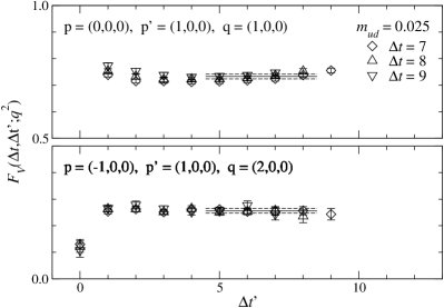
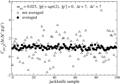
Figure 2: Left panel : effective value $F_{V}(\Delta t,\Delta t^{\prime};q^{2})$ at $m_{ud}\!=\!0.025$, which is around a quarter of the physical strange quark mass. Right panel : statistical fluctuation of $C_{\pi V_{4}\pi}(\Delta t,\Delta t^{\prime};{\bf p},{\bf p}^{\prime})$ at $(|{\bf p}|,|{\bf p}^{\prime}|)\!=\!(\sqrt{2},0)$ and $\Delta t\!=\!\Delta t^{\prime}\!=\!7$. Filled and open symbols are results with and without averaging over the source location $({\bf x},t)$.

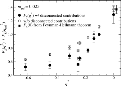
Figure 3: Left panel: effective value of normalized scalar form factor $F_{S}(\Delta t,\Delta t^{\prime};q^{2})/F_{S}(\Delta t,\Delta t^{\prime};q_{\rm ref}^{2})$ at $m_{ud}\!=\!0.025$. Right panel: scalar form factor $F_{S}(q^{2})$ with (filled symbols) and without (open symbols) the contributions of the disconnected diagrams . Both data are normalized by a common value $F_{S}(q_{\rm ref}^{2})$ including the disconnected contribution.

The scalar form factor normalized at a certain momentum transfer $q_{\rm ref}^{2}$ can be calculated from

$$\frac{F_{S}(\Delta t,\Delta t^{\prime};q^{2})}{F_{S}(\Delta t,\Delta t^{\prime};q_{\rm ref}^{2})} = \frac{R_{S}(\Delta t,\Delta t^{\prime};q^{2})}{R_{S}(\Delta t,\Delta t^{\prime};q_{\rm ref}^{2})},$$ (8)

$$R_{S}(\Delta t,\Delta t^{\prime};q^{2}) = \frac{1}{N_{|{\bf p}|,|{\bf p}^{\prime}|}}\sum_{\mbox{\scriptsize fixed }|{\bf p}|,|{\bf p}^{\prime}|}\frac{C_{\pi S\pi}(\Delta t,\Delta t^{\prime};{\bf p},{\bf p}^{\prime})}{C_{\pi\pi}(\Delta t;{\bf p})\,C_{\pi\pi}(\Delta t^{\prime};{\bf p}^{\prime})}.$$ (9)

At $q^{2}\!=\!0$, $C_{\pi S\pi}$ has an additional contribution shown in Fig. 1 due to the VEV of the scalar operator $S$. The subtraction of this contribution leads to a relatively large uncertainty in $F_{S}(\Delta t,\Delta t^{\prime};q^{2})$ at $q^{2}\!=\!0$ than at $q^{2}\!\neq\!0$, as seen in the left of Fig. 3. Although the Feynman-Hellmann theorem $2F_{S}(0)\!=\!\partial M_{\pi}^{2}/\partial m_{ud}$ provides a better determination of $F_{S}(0)$, it is subject to systematic uncertainties of the chiral extrapolation of $M_{\pi}^{2}$. In our simulation setup, $F_{S}(q^{2})$ has the smallest relative error at the smallest nonzero value of $|q_{\rm ref}^{2}|$ with $|{\bf q}_{\rm ref}|\!=\!1$. We therefore use $F_{S}(q^{2})$ normalized at this $q_{\rm ref}^{2}$ in the following analysis.

We determine $F_{S}(q^{2})/F_{S}(q_{\rm ref}^{2})$ from the effective value $F_{S}(\Delta t,\Delta t^{\prime};q^{2})/F_{S}(\Delta t,\Delta t^{\prime};q_{\rm ref}^{2})$ in a similar way to $F_{V}(q^{2})$. The right panel of Fig. 3 compares $F_{S}(q^{2})$ to that without the contribution of the disconnected diagrams. We observe a significant deviation between the two data, which implies the importance of the disconnected contributions in a precision study of $F_{S}(q^{2})$.

4 Parametrization of $q^{2}$ dependence

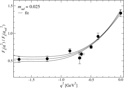
Figure 4: Vector form factor $F_{V}(q^{2})$ (left panel) and normalized scalar form factor $F_{S}(q^{2})/F_{S}(q_{\rm ref}^{2})$ (right panel) as a function of $q^{2}$. Solid lines show the fit curve and its error. We also plot the $q^{2}$ dependence of $F_{V}(q^{2})$ expected from the VMD model by the dashed line.

In Fig. 4, we plot the vector form factor $F_{V}(q^{2})$ and normalized scalar form factor $F_{S}(q^{2})/F_{S}(q_{\rm ref}^{2})$ as a function of $q^{2}$. We observe that $F_{V}(q^{2})$ is close to the vector meson dominance (VMD) hypothesis $1/(1-q^{2}/M_{\rho}^{2})$ with the vector meson mass $M_{\rho}$ measured at simulated $m_{ud}$. We then assume that the small deviation due to the higher poles or cuts can be approximated by a polynomial of $q^{2}$. The $q^{2}$ dependence of $F_{V}(q^{2})$ is therefore parametrized as

$$F_{V}(q^{2}) = \frac{1}{1-q^{2}/M_{\rho}^{2}}+a_{V,1}\,q^{2}+a_{V,2}\,(q^{2})^{2}+a_{V,3}\,(q^{2})^{3}\hskip 2.84526pt=\hskip 2.84526pt1+\frac{1}{6}\langle r^{2}\rangle_{V}q^{2}+c_{V}(q^{2})^{2}+\cdots\hskip 14.22636pt$$ (10)

in order to determine the charge radius $\langle r^{2}\rangle_{V}$ and the curvature $c_{V}$. This form describes our data well as shown in Fig. 4. Results for $\langle r^{2}\rangle_{V}$ and $c_{V}$ do not change significantly if we remove the cubic term or if we add higher order terms into the parametrization form.

Due to the lack of the knowledge about the scalar resonances at the simulated quark masses, we use a generic quartic form

$$F_{S}(q^{2}) = F_{S}(0)\left(1+\frac{1}{6}\langle r^{2}\rangle_{S}\,q^{2}+c_{S}(q^{2})^{2}+a_{S,3}\,(q^{2})^{3}+a_{S,4}\,(q^{2})^{4}\right)$$ (11)

to parametrize the $q^{2}$ dependence of $F_{S}(q^{2})$. Our data are described by this form reasonably well as in Fig. 4. The result for the scalar radius $\langle r^{2}\rangle_{S}$ is stable against the removal of the the quartic term as well as inclusion of higher order terms. Such a stability is, however, not clear in the curvature $c_{S}$ due to its large statistical uncertainty. We leave a precise determination of $c_{S}$ for future studies, and only use results for $\langle r^{2}\rangle_{S}$ in the following analysis.

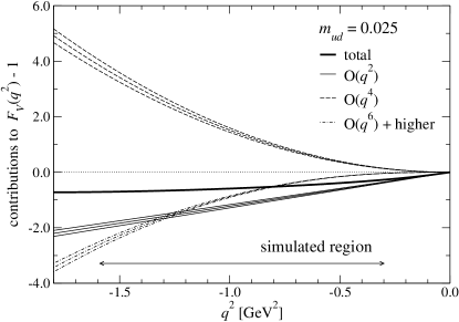
Figure 5: Contributions in the $q^{2}$ expansion of $F_{V}(q^{2})\!-\!1$ at $m_{ud}\!=\!0.025$. Thin solid, dashed and dot-dashed lines show $O(q^{2})$, $O(q^{4})$ and higher order contributions. The thick solid line is their total.

ChPT can provide a more unambiguous parametrization of $F_{V,S}(q^{2})$. Figure 5 shows contributions to $F_{V}(q^{2})$ from each order $(q^{2})^{n}$ of a Taylor expansion of Eq. (10). We observe that $O(q^{6})$ and higher order contributions, which are NNNLO and higher in ChPT, become a small (a few %) correction below $|q^{2}|\!\lesssim\!(550\mbox{MeV})^{2}$. Our values of $|q^{2}|$ are, however, outside of this region due to the use of the simple periodic boundary condition for quark fields. We therefore do not use a parametrization of the $q^{2}$ dependence based on ChPT in this study.

We note that the simulated values of the pion mass squared $M_{\pi}^{2}$ are smaller than $(520\,\mbox{MeV})^{2}$. The $O(q^{6})$ contribution to $F_{V}(q^{2})$ is small if $|q^{2}|$ is smaller than this value. The quark mass dependence of our data of $\langle r^{2}\rangle_{V,S}$ is expected to be described by NNLO ChPT.

5 Chiral extrapolation

We first compare our lattice data of the radii $\langle r^{2}\rangle_{V,s}$ with NLO ChPT formulae [9]

$$\langle r^{2}\rangle_{V}=-\frac{1}{NF^{2}}\left(1+6N\,l_{6}^{r}\right)-\frac{1}{NF^{2}}\ln\left[\frac{M_{\pi}^{2}}{\mu^{2}}\right],\hskip 5.69054pt\langle r^{2}\rangle_{S}=\frac{1}{NF^{2}}\left(-\frac{13}{2}+6N\,l_{4}^{r}\right)-\frac{6}{NF^{2}}\ln\left[\frac{M_{\pi}^{2}}{\mu^{2}}\right],\hskip 28.45274pt$$ (12)

where $N\!=\!(4\pi)^{2}$ and $F$ is the decay constant in the chiral limit. We fix $F$ to our estimate from our study of the pion decay constant [10]. The renormalization scale is set to $\mu\!=\!4\pi F$. The NLO fits are not quite successful as seen in Fig. 6. While our data of $\langle r^{2}\rangle_{V}$ are fitted well with $\chi^{2}/{\rm d.o.f.}\!\sim\!0.1$, the value extrapolated to the physical quark mass $0.364(4)~{}\mbox{fm}^{2}$ is significantly smaller than experiment [12]. On the other hand, the NLO formula for $\langle r^{2}\rangle_{S}$ with the enhanced chiral log fails to reproduce our data and leads to large $\chi^{2}/{\rm d.o.f.}\!\sim\!9$.

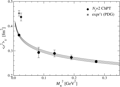
Figure 6: Chiral fit of $\langle r^{2}\rangle_{V}$ (left panel) and $\langle r^{2}\rangle_{S}$ (right panel) using NLO ChPT formulae. In the left panel, we also plot the experimental value $\langle r^{2}\rangle_{V}\!=\!0.437(16)~{}\mbox{fm}^{2}$ from an analysis based on $N_{f}\!=\!2$ ChPT [11] (diamond) and $0.452(11)~{}\mbox{fm}^{2}$ quoted by Particle Data Group [12] (star). The diamond in the right panel represents $\langle r^{2}\rangle_{S}\!=\!0.61(4)~{}\mbox{fm}^{2}$ obtained from an indirect determination through $\pi\pi$ scattering [13].

We also note that NLO in ChPT is not sufficient to describe the quark mass dependence of the curvature $c_{V}$. Although $c_{V}$ has a NLO term $1/(60NF^{2}M_{\pi}^{2})$ coming from non-analytic NLO contributions to $F_{V}(q^{2})$, it dominates $c_{V}$ well below the physical pion mass and fairly near the chiral limit (see Fig. 7 below), where the non-analytic contributions to $F_{V}(q^{2})$ are important to be consistent with the existence of the $\gamma\to\pi\pi$ branch cut at $q^{2}\!\gtrsim\!0$. Since $c_{V}$ characterizes the $O(q^{4})$ dependence of $F_{V}(q^{2})$, NNLO contributions are essential to describe its quark mass dependence.

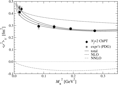
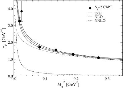
Figure 7: Simultaneous chiral fit to $\langle r^{2}\rangle_{V}$ and $c_{V}$ based on two-loop formulae Eqs. (13) and (15). We also plot a phenomenological estimate $c_{V}\!=\!3.85(60)$ [11].

We therefore extend our analysis to NNLO ChPT. The NNLO contributions to the radii are [11, 14]

$$\Delta\langle r^{2}\rangle_{V} = \frac{1}{N^{2}F^{4}}\left(\frac{13N}{192}-\frac{181}{48}+6N^{2}r_{V,r}^{r}\right)\,M_{\pi}^{2}+\frac{1}{N^{2}F^{4}}\left(\frac{19}{6}-12Nl_{1,2}^{r}\right)\,M_{\pi}^{2}\ln\left[\frac{M_{\pi}^{2}}{\mu^{2}}\right],$$ (13)

$$\Delta\langle r^{2}\rangle_{S} = \frac{1}{N^{2}F^{4}}\left(-\frac{23N}{192}+\frac{869}{108}+88Nl_{1,2}^{r}+80Nl_{2}^{r}+5Nl_{3}^{r}-24N^{2}l_{3}^{r}l_{4}^{r}+6N^{2}r_{S,r}^{r}\right)\,M_{\pi}^{2}$$ (14)

$$+\frac{1}{N^{2}F^{4}}\left(-\frac{323}{36}+124Nl_{1,2}^{r}+130Nl_{2}^{r}\right)\,M_{\pi}^{2}\ln\left[\frac{M_{\pi}^{2}}{\mu^{2}}\right]-\frac{65}{3N^{2}F^{4}}M_{\pi}^{2}\ln\left[\frac{M_{\pi}^{2}}{\mu^{2}}\right]^{2}.$$

The NNLO expression of $c_{V}$ is

$$c_{V} = \frac{1}{60NF^{2}}\frac{1}{M_{\pi}^{2}}+\frac{1}{N^{2}F^{4}}\left(\frac{N}{720}-\frac{8429}{25920}+\frac{N}{3}l_{1,2}^{r}+\frac{N}{6}l_{6}^{r}+N^{2}r_{V,c}^{r}\right)$$ (15)

$$+\frac{1}{N^{2}F^{4}}\left(\frac{1}{108}+\frac{N}{3}l_{1,2}^{r}+\frac{N}{6}l_{6}^{r}\right)\,\ln\left[\frac{M_{\pi}^{2}}{\mu^{2}}\right]+\frac{1}{72N^{2}F^{4}}\ln\left[\frac{M_{\pi}^{2}}{\mu^{2}}\right]^{2}.$$

The analytic terms with $r_{\{V,S\},\{r,c\}}^{r}$ represent contributions from $O(p^{6})$ chiral Lagrangian. The linear combination $l_{1}^{r}\!-\!l_{2}^{r}/2$ appearing commonly in $\langle r^{2}\rangle_{V}$ and $c_{V}$ is denoted by $l_{1,2}^{r}$ for simplicity.

We first carry out a simultaneous fit to $\langle r^{2}\rangle_{V}$ and $c_{V}$ in terms of $M_{\pi}^{2}/(NF^{2})$. This fit has only four free parameters $l_{6}^{r}$, $l_{1,2}^{r}$, $r_{V,r}^{r}$ and $r_{V,c}^{r}$ [3], and these can be determined with reasonable accuracy without introducing phenomenological inputs. As seen in Fig. 7, our data are well described by the NNLO formulae with $\chi^{2}/{\rm d.o.f.}\!\sim\!0.7$. The extrapolated values of $\langle r^{2}\rangle_{V}$ and $c_{V}$ are consistent with recent phenomenological determinations [11, 15, 16].

The inclusion of $\langle r^{2}\rangle_{S}$ into the simultaneous fit introduces additional four free parameters $l_{2}^{r}$, $l_{3}^{r}$, $l_{4}^{r}$ and $r_{S,r}^{r}$, and we need to fix some of them to obtain a stable fit. In this study, we use a phenomenological estimate $\bar{l}_{2}\!=\!4.31(11)$ [13] and a lattice estimate $\bar{l}_{3}\!=\!3.38(56)$ from our analysis of the pion mass [10] , since they are determined with a reasonable accuracy and appear only in the NNLO terms. As plotted in Fig. 8, this fit describes our data of $\langle r^{2}\rangle_{S}$ reasonably well with $\chi^{2}/{\rm d.o.f.}\!\sim\!0.7$. The extrapolations of $\langle r^{2}\rangle_{V}$ and $c_{V}$ are consistent with those in Fig. 7.

At physical quark mass, we obtain

$$\langle r^{2}\rangle_{V}=0.409(23)(37)~{}\mbox{fm}^{2},\hskip 5.69054pt\langle r^{2}\rangle_{S}=0.617(79)(66)~{}\mbox{fm}^{2},\hskip 5.69054ptc_{V}=3.22(17)(36)~{}\mbox{GeV}^{-4},\hskip 5.69054pt$$ (16)

where the first and second errors are statistical and systematic, respectively. The latter includes uncertainties due to the choice of the input to fix the lattice scale and the inputs for the LECs ($F$, $l_{2}$ and $l_{3}$) as well as uncertainties due to the chiral extrapolation and lattice discretization. These results for $\langle r^{2}\rangle_{V,S}$ and $c_{V}$ are consistent with phenomenological analyses.

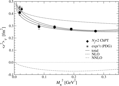
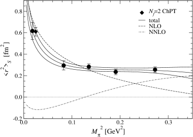
Figure 8: Chiral extrapolation of radii $\langle r^{2}\rangle_{V,S}$ obtained from simultaneous fit to $\langle r^{2}\rangle_{V,S}$ and $c_{V}$.

The results for the relevant LECs are

$$\bar{l}_{6}=11.9(0.7)(1.0),\hskip 8.53581pt\bar{l}_{4}=4.09(50)(52),\hskip 8.53581pt\bar{l}_{1}-\bar{l}_{2}=-2.9(0.9)(1.3),$$ (17)

$$r_{V,r}^{r}=-1.0(1.0)(2.5)\times 10^{-5},\hskip 8.53581ptr_{V,c}^{r}=4.00(17)(64)\times 10^{-5},\hskip 8.53581ptr_{S,r}^{r}=1.74(36)(78)\times 10^{-4}.\hskip 28.45274pt$$ (18)

Our estimate of $\bar{l}_{6}$ is slightly smaller than those from ChPT analyses: $\bar{l}_{6}\!=\!16.0(0.9)$ from $F_{V}$ [11] and 15.2(0.4) from $\tau$ and $\pi$ decays [17]. This is partly because our estimate of $F$ [10] is slightly smaller than phenomenological estimates. We note that $\bar{l}_{4}$ is consistent with our determination $\bar{l}_{4}\!=\!4.12(56)$ from $F_{\pi}$ [10] and a phenomenological estimate 4.39(22) [13].

6 Conclusions

In this article, we present our calculation of pion form factors in two-flavor lattice QCD with exact chiral symmetry, which enables us to unambiguously compare our lattice data with two-loop ChPT. By employing the all-to-all quark propagators, $F_{S}(q^{2})$ is calculated including contributions from the disconnected diagrams for the first time. We observe that two-loop contributions are important to describe the quark mass dependence of $\langle r^{2}\rangle_{V,S}$ and $c_{V}$ at our region of the pion mass $M_{\pi}\!\gtrsim\!290$ MeV. Our chiral extrapolation of $\langle r^{2}\rangle_{V,S}$ and $c_{V}$ are consistent with phenomenological analyses. We also confirm that $F_{S}(q^{2})$ and $F_{\pi}$ lead to consistent results for $l_{4}$.

For a more precise comparison with experiment, we need to extend this study to three-flavor QCD. Such simulations are currently underway. Another important subject is a better control of the parametrization of the $q^{2}$ dependence of $F_{V,S}(q^{2})$. To this end, the use of the twisted boundary condition [18] to simulate small values of $|q^{2}|$, dispersive analysis of the $q^{2}$ dependence [15, 16], and model-independent determination of the scalar resonance mass [19] are interesting possibilities for our future studies.

I am grateful to my colleagues in the JLQCD and TWQCD collaborations. I also thank Balasubramanian Ananthanarayan and Sunethra Ramanan for a useful correspondence. Numerical simulations are performed on Hitachi SR11000 and IBM System Blue Gene Solution at High Energy Accelerator Research Organization (KEK) under a support of its Large Scale Simulation Program (No. 08-05). This work is supported in part by the Grant-in-Aid of the Ministry of Education (No. 20105005 and 21684013).

References

[1]
R. Narayanan and H. Neuberger,
Nucl. Phys. B 443, 305 (1995).
[2]
J. Foley et al. (TrinLat collaboration),
Comput. Phys. Commun, 172, 145 (2005).
[3]
S. Aoki et al. (JLQCD and TWQCD collaborations),
Phys. Rev. D 80, 034508 (2009).
[4]
H. Fukaya et al. (JLQCD collaboration),
Phys. Rev. D 74, 094505 (2006).
[5]
S. Aoki et al. (JLQCD collaboration),
Phys. Rev. D 78, 014508 (2008).
[6]
S.-J. Dong and K.-F. Liu,
Phys. Lett. B 328, 130 (1994).
[7]
S. Hashimoto et al.,
Phys. Rev. D 61, 014502 (1999).
[8]
T.B. Bunton, F.-J. Jiang and B.C. Tiburzi,
Phys. Rev. D 74, 034514 (2006).
[9]
J. Gasser and H. Leutwyler,
Ann. Phys. 158, 142 (1984).
[10]
J. Noaki et al. (JLQCD and TWQCD collaborations),
Phys. Rev. Lett. 101, 202004 (2008).
[11]
J. Bijnens, G. Colangelo and P. Talavera,
JHEP 9805, 014 (1998).
[12]
C. Amsler et al. (Particle Data Group),
Phys. Lett. B 667, 1 (2008).
[13]
G. Colangelo, J. Gasser and H. Leutwyler,
Nucl. Phys. B 603, 125 (2001).
[14]
J. Gasser and U.-G. Meißner,
Nucl. Phys. B 357, 90 (1991).
[15]
B. Ananthanarayan and S. Ramanan,
Eur. Phys. J. C 60, 73 (2009).
[16]
F.-K. Guo et al.,
arXiv:0812.3270 [hep-ph].
[17]
M. González-Alonso, A. Pich and J. Prades,
Phys. Rev. D 78, 116012 (2008).
[18]
P.F. Bedaque,
Phys. Lett. B 593, 82 (2004).
[19]
I. Caprini, G. Colangelo and H. Leutwyler,
Phys. Rev. Lett. 96, 132001 (2006).