Characterization of Stellar Spots in Next-Generation Microlensing Surveys

Abstract

One of the important microlensing applications to stellar atmospheres is the study of spots on stellar surface provided by the high resolution of caustic-crossing binary-lens events. In this paper, we investigate the characteristics of spot-induced perturbations in microlensing light curves and explain the physical background of the characteristics. We explore the variation of the spot-induced perturbations depending on various parameters characterizing the spot and investigate how well these parameters can be retrieved from observations in high-cadence future lensing surveys. From this, we find that although it would not be easy to precisely constrain the shape and the surface brightness contrast, the size and location of the spot on the stellar surface can be fairly well constrained from the analysis of lensing light curves.

1. Introduction

Over the past decade, microlensing has developed into a powerful tool to study stellar astrophysics, especially stellar atmospheres. See the review of Gould (2001). Microlensing application to stellar atmosphere is possible for events where the source star crosses the caustic. The caustic represents the source position at which the lensing magnification of a point source formally becomes infinity. Then, as the caustic passes over the face of the star, different parts of the star are strongly magnified at different times, making it possible to probe detailed structures on the surface of the source star. One of the stellar properties that can be investigated by the high resolution provided by caustic-crossing microlensing events is the limb darkening of stars (Witt, 1995; Bogdanov & Cherepashchuk, 1995; Gaudi & Gould, 1999; Albrow et al., 1999, 2001; Afonso et al., 2000; Gould, 2001; Heyrovský, 2003; Fields et al., 2003; Abe et al., 2003; Dominik, 2004; Kubas et al., 2005; Cassan et al., 2006).

Another application of microlensing to stellar atmosphere is the study of irregular surface structures such as spots. Heyrovský & Sasselov (2000) and Hendry, Bryce & Valls-Gabaud (2002) investigated the sensitivity to spots for single-lens events and found that the spot signal can be detected for events where the lens transits the face of the source star. Han et al (2000) and Chang & Han (2002) demonstrated the feasibility of spot detections from the observation of caustic-crossing binary-lens events.

Despite the feasibility of spot detections demonstrated by theoretical studies, there exists no firm detection of a spot signal for any of the microlensing events detected so far. This might be due to the small fraction of stars with spots, but it is more likely that the current lensing surveys are not sensitive enough to catch the signal. For a caustic-crossing binary-lens event, the duration of a spot-induced signal is

$$t_{\bullet}\sim\iota_{\bullet}{2\rho_{\star}\over\sin\phi}t_{\rm E},$$ (1)

where $\iota_{\bullet}$ is the fraction of the spot size relative to the source size, $\rho_{\star}$ is the source radius normalized by the Einstein radius $\theta_{\rm E}$, $t_{\rm E}$ is the Einstein time scale, and $\phi$ is the angle between the source trajectory and the caustic line. Considering that $t_{\rm E}\sim 20$ days for a typical Galactic event, the time scale is

$$t_{\bullet}\sim 0.12\ \left({\iota_{\bullet}\over 0.1}\right)\left({R_{\star}\over R_{\odot}}\right)\ {\rm hrs}.$$ (2)

Then, the spot-induced perturbation lasts only a few hours even for an event associated with a giant source star. On the other hand, the observational cadence of the current lensing surveys is several times per night, which is far less than that required to detect the spot-induced perturbations.

However, the situation will be greatly different in future lensing surveys that will continuously survey wide fields at a high cadence using very large format imaging cameras. The OGLE collaboration recently upgraded their camera to widen the field of view from $0.4\ {\rm deg}^{2}$ to $1.4\ {\rm deg}^{2}$. The MOA collaboration plans to upgrade the telescope to a field of view of $4\ {\rm deg}^{2}$ (T. Sumi 2009, private communication). The ‘Korea Microlensing Telescope Network (KMTNet)’ is a survey exclusive for microlensing that plans to achieve $\sim$ 10 minute sample using a network of three 1.6 m telescopes each of which is equipped with a camera of a $4\ {\rm deg}^{2}$ field of view. With these upgraded and new instruments, the next-generation surveys will be able to resolve the short time-scale perturbations induced by spots.

In this paper, we further explore the feasibility of microlensing studies of stellar spots. We investigate the characteristics of spot-induced perturbations in microlensing light curves and explain the physical background of the characteristics. We also investigate the feasibility of constraining the physical parameters of spots from the observations in future lensing surveys.

2. Spot-Induced Perturbations

2.1. Characteristics

Figure 1 shows the light curve of an example caustic-crossing binary-lens event occurring on a source star with a spot and the resulting pattern of the spot-induced perturbation. From the investigation of the perturbation, one finds the two following important characteristics of the perturbation pattern. First, there exist both positive and negative deviations in lensing magnification from the light curve of the event occurring on an unspotted star. Second, the perturbation pattern is asymmetric with respect to the maximum deviation.

For an event occurred on a spotted star, the lensing magnification is represented by

$$A_{\bullet}={\int_{\Sigma_{\star}}A(x,y)dxdy-(1-C_{\rm s})\int_{\Sigma_{\bullet}}A(x,y)dxdy\over\Sigma_{\star}-\Sigma_{\bullet}},$$ (3)

where $A(x,y)$ represents the point-source magnification at a source position $(x,y)$, $C_{\rm s}$ is the flux ratio between the spot and unspotted regions, and $\Sigma_{\star}$ and $\Sigma_{\bullet}$ represent the surface areas of the star and the spot, respectively. Here we assume that the brightness distribution on the source star surface other than the spot region is uniform. Then, the first term of the numerator of the right side of equation (3) represents the contribution of the unspotted region to the magnification (non-spot term), while the second term represents the contribution of the spot region (spot term).

The negative deviation in the spot-induced perturbation occurs when the magnification of the spot region is very high. In this case, the decrease of the numerator in equation (3) by the spot term is more important than the decrease of the denominator by the spot area, resulting in a negative deviation. The magnification of the spot region is maximized when the spot is on the caustic.

The positive deviation occurs when the caustic is over the source surface but the spot is away from the caustic. In this case, the magnification at the position of the spot is not high and the non-spot term in equation (3) dominates over the spot term. Then, the decrease in the numerator is negligible while the decrease of the denominator remains the same regardless of the spot position. With the increment of the denominator, the magnification is higher than the magnification of an unspotted event, resulting in a positive deviation.

The asymmetry of the perturbation pattern is caused by the difference in magnification patterns between the outside and the inside regions of the caustic. In the outer region, the magnification plummets as the distance $d$ from the caustic increases, while the magnification inside the caustic decreases smoothly as $A\propto d^{-1/2}$. Then, the spot term in equation (3) is important in a very narrow region outside of the caustic but in a much wider region inside the caustic. As a result, the deviation pattern is asymmetric.

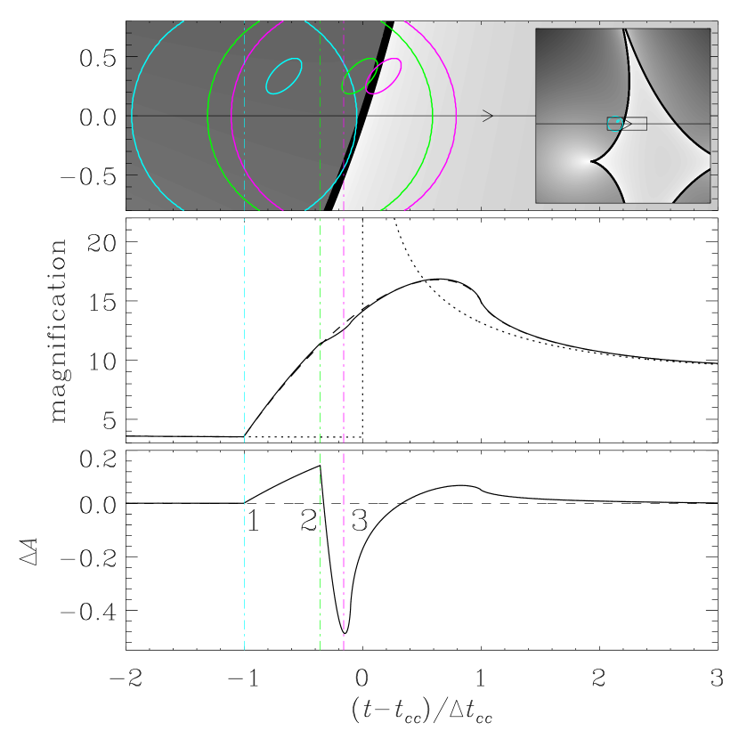
Figure 1.— Light curve of a caustic-crossing binary-lens event occurred on a source star with a spot (middle panel) and the the residual from that of the event occurring on an unspotted source star (lower panel). The light curve is in lensing magnification and the residual is the difference in magnification. The upper panel shows the geometry of the lens system where the thick linear structure represents the caustic and the straight line with an arrow represents the source trajectory. The grey scale shows the point-source magnification as a function of position and brighter tone represents a higher magnification. The inset shows the wider view of the geometry. The circles with different colors represents the source at the times marked by numbers in the lower panel. The spot of each source is also marked. The three light curves in the middle panel represent those of events occurred on source stars with a spot (solid curve), without a spot (dashed curve), and a point source (dotted curve), respectively. The time is expressed with respect to the time of the caustic crossing of the source center, $t_{cc}$, in units of the caustic-crossing time scale $\Delta t_{cc}$.

With the understanding of the physical background of the patterns of spot-induced perturbations, the locations of several important turning points in the perturbation can be explained. For the case of the example event presented in Figure 1, there exist three such points, each of which is marked by a number.

1. The position marked by “1” corresponds to the moment at which the source surface enters the caustic. Differential magnification becomes important from this moment. The highly magnified parts on the source star surface are unspotted regions and thus the non-spot terms dominates over the spot term, resulting in a positive deviation.

2. The position marked by “2” corresponds to the moment of spot’s entrance into the caustic. From this moment, the spot term becomes important and the deviation rapidly drops into negative values.

3. The negative deviation is maximized when the spot term is maximized and this corresponds to the position marked by “3”. We note that the magnification inside and outside of the caustic is very different and thus the moment of maximum negative deviation occurs not at the moment when the center of the spot is exactly on the caustic but when the center is slightly shifted toward the inside of the caustic.

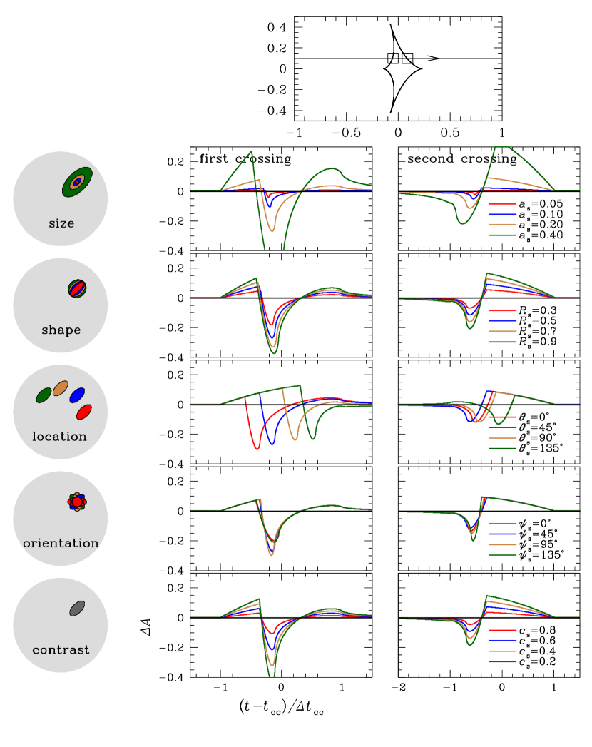
Figure 2.— Variation of the spot-induced perturbations. The top panel shows the geometry of the lens system with respect to the caustic produced by a binary lens system with a mass ratio $q=0.5$ and a projected separation normalized by the Einstein radius between the components of $s=0.7$. The source radius relative to the Einstein radius is $\rho_{\star}=0.02$. The subsequent panels show the variation depending on the spot size, the shape, the location, the orientation, and the contrast in brightness between the spot and unspotted regions, respectively.

2.2. Variation

Based on the fundamental scheme of the deviation described in the previous subsection, spot-induced perturbations take different shapes depending on various factors. These factors include the size, shape, location on the source surface, orientation, brightness contrast with respect to the unspotted region, etc.

Figure 2 shows how the spot-induced perturbation depends on various factors. Under the simplified approximation of a single elliptical spot with a uniform surface brightness, we parameterize the spot size as the semi-major axis $a_{\rm s}$ normalized by the source radius, the shape as the axis ratio $R_{\rm s}$ of the ellipse, the location on the source as the polar coordinates ($r_{\rm s}$, $\theta_{\rm s}$) of the center of the ellipse with respect to the source center, the orientation as the angle $\psi_{\rm s}$ between the semi-major axis of the spot and the source trajectory, and the brightness contrast as the flux ratio $C_{\rm s}$ between the spot and unspotted regions.

3. Characterization

In the previous section, we explored the variation of the pattern of spot-induced perturbations depending on various parameters that characterize the spot. In this section, we investigate how well these parameters can be retrieved from the analysis of light curves of event to be observed in future lensing surveys. For this, we estimate the uncertainties of the spot parameters by fitting an example caustic-crossing binary-lens event produced by simulation under the observational conditions of planned future lensing surveys.

We choose the lensing parameters of the example event by adopting those of a typical Galactic bulge event occurred on a giant star. The adopted values of the Einstein time scale is $t_{\rm E}=20$ days. The projected separation normalized by the Einstein radius and the mass ratio between the lens components are $s=0.7$ and $q=0.5$, respectively. The apparent baseline magnitude of the source is $I=15$ and the fraction of the flux from the lensed star is 70% and the rest comes from blended stars. The source trajectory with respect to the caustic is same as shown in the top panel of Figure 2. The values of the parameters characterizing the spot properties are $a_{\rm s}=0.3$, $R_{\rm s}=0.5$, $\psi_{\rm s}=45^{\circ}$, $r_{\rm s}=0.5$, $\theta_{\rm s}=45^{\circ}$, and $C_{\rm s}=0.5$.

The event is assumed to be continuously observed in the $I$ passband by using a network of telescopes with a cadence of 6 times per hour. The exposure of each observation is 30 seconds. The aperture of each telescope is 1.6 m and the quantum efficiency of the detector is 0.8. Given the specification of the instrument and the magnitude of the source and blend, we set the photometric uncertainty by assuming that the photometry follows photon statistics with a 1% systematic uncertainty. We also assume that the photometry is Gaussian distributed. Figure 3 shows the caustic-crossing part of the light curve produced by the simulation (upper panel) and the residual from the unspotted light curve (lower panel).

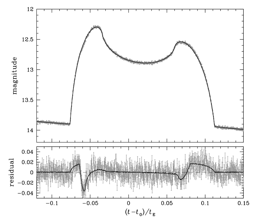
Figure 3.— Light curve of the event produced by simulation that is used for the estimation of the uncertainties of the spot parameters. We note that the light curve is expressed in magnitude. The time $t_{0}$ represents the moment of the closest approach of the source star to the center of mass of the binary lens.

The uncertainties of the spot parameters are estimated by fitting the light curve produced by simulation. In the fitting process, we search for a set of parameters describing the perturbation by minimizing $\chi^{2}$ in the parameter space. We use a Markov Chain Monte Carlo method for the $\chi^{2}$ minimization. Since a spot-induced perturbation occurs in a small region during the caustic crossing, its effect on the other lensing parameters is negligible. We, therefore, set the lensing parameters fixed in the fitting process. We hold two of the spot parameters fixed at a grid of values, while the remaining parameters are allowed to vary so that the model light curve results in a minimum $\chi^{2}$ at each grid point. We set $a_{\rm s}$ and $R_{\rm s}$ as the grid parameters because they characterize the two most important properties of a spot. Another important reason for using grid parameters is that it allows to use multiple CPUs by allocating computations of different sections of the grid-parameter space different CUPs. Once a series of models for the individual sets of the grid parameters are obtained, we estimate the uncertainty of each parameter from the distribution of the parameter obtained by giving weight to the $\chi^{2}$ difference from the value of the best-fit model.

For the computation of lensing magnification affected by spot perturbation, we use the ray-shooting technique (Schneider & Weiss, 1986; Kayser, Refsdal, & Stabell, 1986; Wambsganss, 1997). In this technique, a large number of light rays are uniformly shot from the observer plane through the lens plane and then collected on the source plane. We accelerate this process by restricting the region of ray-shooting only in the region around the caustic and using a simple semi-analytic approximation in other parts of the source plane. In addition, we keep the information of the positions of the light rays arriving at the target in the buffer memory of the computer so that it can be readily used for fast computation of the magnification.

Table 1Uncertainties of Spot Parameters

property	parameter	uncertainty
semi-major axis	$a_{\rm s}$	$\sigma_{a_{\rm s}}=0.04$
axis ratio	$R_{\rm s}$	$\sigma_{R_{\rm s}}=0.2$
orientation	$\psi_{\rm s}$	$\sigma_{\psi_{\rm s}}=30^{\circ}$
location of the source surface	$(r_{\rm s},\theta_{\rm s})$	$(\sigma_{r_{\rm s}},\sigma_{\theta_{\rm s}})=(0.02,5^{\circ})$
surface-brightness contrast	$C_{\rm s}$	$\sigma_{C_{\rm s}}=0.4$

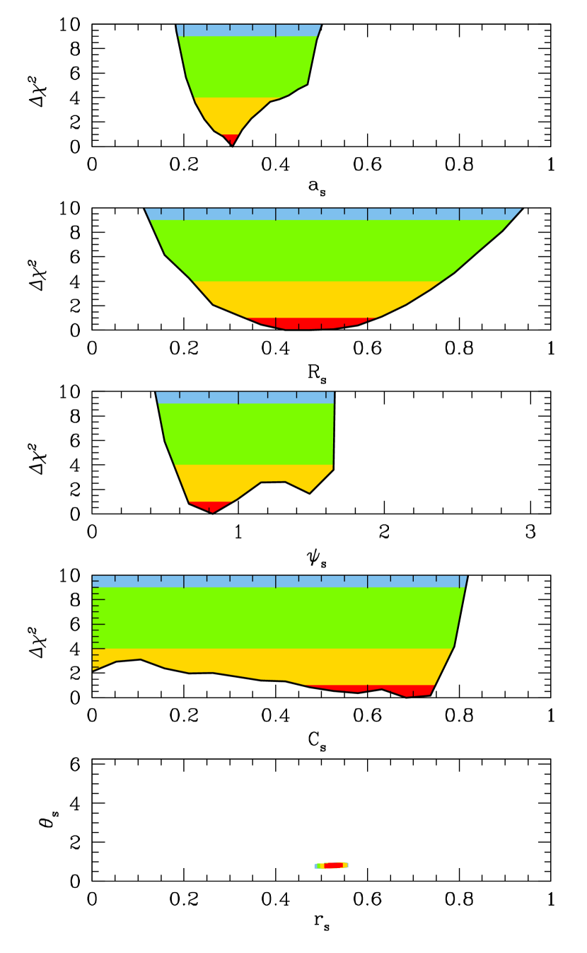
Figure 4.— Distributions of $\Delta\chi^{2}$ for the spot parameters. The regions marked in red, yellow, and green regions represent those of $\Delta\chi^{2}\leq 1$, 4, and 9, respectively.

We present the distributions of $\Delta\chi^{2}$ for the individual parameters in Figure 4 and list the determined uncertainties in Table 1. From the uncertainties, we find the following factors. First, the size of the spot can be well constrained with uncertainties of $\sigma_{a_{\rm s}}\sim 0.05$. We judge the reason for this is due to the existence of the discrete structures on the spot perturbation such as the turning points mentioned in section 2. These structures depends on the spot size and thus help to constrain the size. Second, the location of the spot on the surface of the source star is also well constrained. This is because the source surface is swept by the caustic two times, i.e. at the entrance and exit. For the individual caustic crossings, the incidence angles of the source respect to the caustic are different and thus the location of the spot is well constrained. On the other hand, the shape of the spot is expected to be determined with a relatively large uncertainty. Same is true for the surface-brightness contrast. This can be understood from the similarity in the variation of the perturbation pattern depending on the two spot parameters of $R_{\rm s}$ and $C_{\rm s}$ as shown in Figure 2, where it is found that the variation of the perturbation with the increase of $R_{\rm s}$ is imitated by the variation with the increase of $C_{\rm s}$. This implies that an observed perturbation suffers from the degeneracy between the two parameters and thus results in large uncertainties of both parameters. The expected uncertainty of the orientation angle of the spot is $\sim 10^{\circ}$.

The uncertainties estimated in this work might be underestimated compared to the actual values in the future experiments. Possible causes of the underestimation would be the simplification of the spot as a uniform ellipse and the disregard of detailed structures such as umbra and pen-umbra. Considering that spots would occupy a small fraction of the source surface and the estimated uncertainty of the spot-size is $\sim 5\%$ of the stellar size, we think that the additional uncertainties caused by the disregard of very detailed structures would not be important. Another cause would be the disregard of the stellar rotation. Due to the stellar rotation, the locations of the spot on the stellar surface at the times of the caustic entrance and exit are different, causing additional uncertainties, especially in $r_{\rm s}$ and $\theta_{\rm s}$. We note, however, that most of the events for which spots can be detected will be events associated with late-type giant source stars for which the angular rotation speed is small. Therefore, the uncertainty would not be seriously different from our estimation.

4. Conclusion

We investigated the characteristics of spot-induced perturbations in microlensing light curves and explained the physical background of the characteristics. We also explored the variation of the spot-induced perturbations depending on various parameters characterizing the spot and investigated how well these parameters can be retrieved from observations in high-cadence future lensing surveys. From this, we found that the size and location of the spot on the stellar surface can be fairly well constrained from the analysis of lensing light curves, although it would not be easy to precisely constrain the shape and the surface brightness contrast

References

- Abe et al. (2003) Abe, F., et al. 2003, A&A, 411, L493
- Albrow et al. (1999) Albrow, M. D., et al. 1999, ApJ, 522, 1011
- Albrow et al. (2001) Albrow, M. D., et al. 2001, ApJ, 549, 759
- Afonso et al. (2000) Afonso, C., et al. 2000, ApJ, 532, 340
- Bogdanov & Cherepashchuk (1995) Bogdanov, M. B., & Cherepashchuk, A. M. 1995, Astronomicheskij Zhurnal, 72, 873
- Cassan et al. (2006) Cassan, A., et al. 2006, A&A, 460, 277
- Chang & Han (2002) Chang, H.-Y., & Han, C. 2002, MNRAS, 335, 195
- Dominik (2004) Dominik, M. 2004, MNRAS, 353, 118
- Fields et al. (2003) Fields, D. L., et al. 2003, ApJ, 596, 1305
- Gaudi & Gould (1999) Gaudi, B. S., & Gould, A. 1999, ApJ, 513, 619
- Gould (2001) Gould, A. 2001, PASP, 113, 903
- Han et al (2000) Han, C., Park, S.-H., Kim, H.-I., & Chang, K. 2000, MNRAS, 316, 665
- Hendry, Bryce & Valls-Gabaud (2002) Hendry, M. A., Bryce, H. M., & Valls-Gabaud, D. 2002, MNRAS, 335, 539
- Heyrovský (2003) Heyrovský, D. 2003, ApJ, 594, 464
- Heyrovský & Sasselov (2000) Heyrovský, D., & Sasselov, D. 2000, ApJ, 529, 69
- Kayser, Refsdal, & Stabell (1986) Kayser, R., Refsdal, S., & Stabell, R. 1986, A&A, 166, 36
- Kubas et al. (2005) Kubas, D., et al. 2005, A&A, 435, 941
- Schneider & Weiss (1986) Schneider, P., & Weiss, A. 1986, A&A, 164, 237
- Wambsganss (1997) Wambsganss, J. 1997, MNRAS, 284, 172
- Witt (1995) Witt, H. J. 1995, ApJ, 449, 42