Quantum attractors of generalized Gauss-Bonnet dark energy

Abstract

The influences of quantum effects on the structure of the phase-space of generalized Gauss-Bonnet theory, introduced by the Lagrangian $F(R,G)$, have been studied. $G$ is the Gauss-Bonnet invariant, and the quantum effects are described via the account of conformal anomaly. It has been shown that the quantum effects change many aspects of the attractors of $F(R,G)$ gravity models in the $R-H$ plane, including the location of the attractors, the number of them and their stability properties. These variations are not, in general, from the type of small perturbations, but instead, it can induce the great, so not ignorable, variations which have root in the ”singular perturbation” nature of this effect. In other words, one can not ignore the quantum corrections and must be always considered. The influences of the perfect barotropic fluids on this problem have been studied, and it has been shown that this kind of matters do not alter the quantum effects. It has been shown that the classical contribution of the coupled-quintessence model, which is responsible for inducing the quantum effects, is of this type, that is a perfect barotropic fluid, and therefore can not change our results.

1 Introduction

Independent observational data indicate that we are now in accelerating phase of the universe. The supernova observations directly support this accelerating expansion, and the microwave background, large scale structure and its dynamics, weak lensing and baryon oscillation observations indirectly verify this phase [1]. It is believed that nearly 70$\%$ of our present universe is composed of dark energy, the physical object which is responsible for the effective negative pressure required for accelerating cosmic expansion.

There are two main dynamical models that explain some features of dark energy. The first one is based on the standard Einstein theory, when some other physical terms added to it. The simple cosmological constant model, with no dynamics [2], the scalar field models, including quintessence, phantom, quintom and hessence models [3], and some other models like the k-essence models, chaplygin gas models, and holographic dark energy models [4] are examples of the first class of dark energy models.

The second class of dark energy models are those based on the assumption that the gravity is being (nowadays) modified. These modified gravity theories can be divided to two main subclasses. The first subclass consists of the models in which, besides the scalar-curvature $R$, there exists a scalar field (or either a vector field) which interacts nonminimally to gravity. These models are known as the scalar-tensor models, where after the simplest Brans-Dicke theory [5], several generalizations have been introduced [6]. Recently it has been shown that the generalized scalar-tensor theories admit the $\omega=-1$ and deceleration to acceleration transitions, the phenomenon which can be affected by quantum effects [7]. The equation of state parameter $\omega$ is defined through $\omega=p/\rho$, where $p$ is the pressure and $\rho$ is the energy density of dark energy. In cosmological constant model, $\omega$ takes the constant value $\omega_{\Lambda}=-1$, and in dynamical models, it is a function of time, i.e. $\omega=\omega(t)$.

The second subclass of modified gravity models are those whose actions are not the simple term $R$, but instead they are, in general, an arbitrary function of all algebraic invariants built up with the Riemann tensor, including the scalar curvature $R$, the quadratic invariants $P=R^{\mu\nu}R_{\mu\nu}$ and $Q=R^{\alpha\beta\gamma\delta}R_{\alpha\beta\gamma\delta}$, and other independent invariants of higher orders. The $f(R)$ gravity, whose Lagrangian is an arbitrary function $f(R)$, is the simplest and the most famous modified gravities of this subclass, i.e.

$$S=\int d^{4}x\sqrt{-g}{}\hskip 4.30554pt\left[\frac{1}{2\kappa^{2}}f(R)+{\cal L}_{m}\right].$$ (1)

In $\hbar=c=G=1$ units, $\kappa^{2}=8\pi$ and ${\cal L}_{m}$ is the Lagrangian density of dust-like matter. Many aspects of $f(R)$ gravity, including their local properties, have been studied. See [8] and references therein.

Restricting ourselves to quadratic invariants, the generalized modified gravity models are defined through

$$S=\int d^{4}x\sqrt{-g}{}\hskip 4.30554pt\left[f(R,P,Q)+{\cal L}_{m}\right],$$ (2)

where $f(R,P,Q)$ is an arbitrary function. Some aspects of these models, including their attractor solutions and their stabilities have been discussed in [9]. Studying the propagators of these models has shown an important result, i.e. the generalized modified gravity models have, in general, the graviton ghost, unless it satisfies [10]

$$\left(f_{P}+4f_{Q}\right)|_{R=R_{0}}=0,$$ (3)

where the subscripts denote the partial derivatives, e.g.

$$f_{P}=\frac{\partial f(R,P,Q)}{\partial P},$$ (4)

and the curvature $R_{0}$ is defined by the equation

$$f-\frac{1}{2}R_{0}f_{R}-\frac{1}{4}{R_{0}}^{2}f_{P}-\frac{1}{6}{R_{0}}^{2}f_{Q}=0.$$ (5)

The above relation is the equation of motion of the metric at constant scalar curvature $R=R_{0}$. In eq.(5), $Q={{R_{0}}^{2}}/{4}$ and $P={{R_{0}}^{2}}/{6}$. Now if one considers the Gauss-Bonnet (GB) invariant $G$

$$G=R^{2}-4P+Q=R^{2}-4R_{\mu\nu}R^{\mu\nu}+R_{\mu\nu\xi\sigma}R^{\mu\nu\xi\sigma}.$$ (6)

it is easily seen that the condition (3) satisfies, and this is a reason why the generalized GB gravity, defined by

$$S=\int d^{4}x\sqrt{-g}{}\hskip 4.30554pt\left[F(R,G)+{\cal L}_{m}\right],$$ (7)

is an important candidate of modified gravity theories.

The generalized GB gravity, where the $f(R)$ gravity (1) is a special example of it, has been first introduced in [11]. The hierarchy problem of particle physics and the late time cosmology in the context of $F(R,G)$, have been studied in [11] and [12], and its behavior under phantom-divide-line crossing and deceleration to acceleration transitions has been investigated in [13]. Recently, the two-dimensional phase-space of the generalized GB models, i.e. the $R-H$ space where $H$ is the Hubble parameter, has been studied in [14] and the various aspects of the de-Sitter attractors of these models have been discussed.

The present paper is devoted to study the contribution of quantum effects to the attractors of generalized GB gravity. The quantum effects are described via the account of conformal anomaly, reminding about anomaly-driven inflation [15]. The contribution of conformal anomaly in energy conditions and big rip of phantom models has been discussed in [16], and its influence on the $\omega=-1$ crossing and deceleration to acceleration transition of quintessence and phantom models, the $F(R,G)$ gravity and the generalized scalar tensor models have been discussed in [17], [13] and [7], respectively.

The late-time behavior of dynamical models, including the dark energy models, is an important problem, both in mathematics and physics, and is studied in a framework known as the attractor solutions of dynamical systems. Many properties of attractor solutions of dark energy models have been studied [18]. Two important parts of attractor studies of any dynamical system are: a) choosing the phase-space of the model and b) obtaining the location of attractors and specifying the stability of them. In $F(R,G)$ gravity models, the only possible choice of phase-space for general $F(R,G)$ model is $R-H$ space. So attractors, with properties $\dot{R}=0$ and $\dot{H}=0$, or $R=R_{c}$ and $H=H_{c}$ ($R_{c}$ and $H_{c}$ are constant values ), are de-Sitter solutions of generalized GB models. Now, as we will show, the quantum effects have important, and non-ignorable, contributions to this problem. It changes the position of the attractors and their stability behaviors, and, for some cases, it produces the new attractors where some of them do not lead to classical attractors, a phenomena known as ”singular perturbation” in mathematics. This shows that the quantum effects are not ignorable, i.e. they do not only lead to small corrections for classical solutions. For some other cases, it can remove the degeneracy of solutions, which is known as ”bifurcation” in the mathematics of dynamical systems. And, interestingly, it can transform the critical curves, an infinite number of stable attractors locating on $R=12H^{2}$ curve in the phase-space of some specific case of $F(R,G)$ models, to a unique point.

The scheme of the paper is as follows: In section 2, we discuss the critical points and the stability conditions of $F(R,G)$ models in the presence of quantum correction terms. It is shown that in the $\hbar\rightarrow 0$ limit, the relations are correctly reduced to classical relations. In section 3, we discuss the various examples of $f(R)$ and $F(R,G)$ models. The new aspects of the phase-space of these models, including those introduced in the last paragraph, can be seen via these examples. It is shown that the numerical calculations verify our results. The usual matter’s contributions to the location and behavior of attractors are discussed in section 4. It is shown that the barotropic fluids can not change the structure of the phase-space of $F(R,G)$ models. It is also shown that the classical contributions of the coupled-quintessence model, which is responsible for producing the quantum correction terms considered in section 2, can not alter our results, which is an important consequence.

2 Quantum corrected critical points of $F(R,G)$ gravity

Consider the generalized GB dark energy with action (7). Variation of this action with respect to the metric $g_{\mu\nu}$ results in [11]

$$\begin{split}&\frac{1}{2}T^{\mu\nu}+\frac{1}{2}g^{\mu\nu}F(R,G)-2F_{G}(R,G)RR^{\mu\nu}+4F_{G}(R,G)R^{\mu}_{~{}\rho}R^{\nu\rho}\\ &-2F_{G}(R,G)R^{\mu\rho\sigma\tau}R^{\nu}_{~{}\rho\sigma\tau}-4F_{G}(R,G)R^{\mu\rho\sigma\nu}R_{\rho\sigma}+2(\nabla^{\mu}\nabla^{\nu}F_{G}(R,G))R\\ &-2g^{\mu\nu}(\nabla^{2}F_{G}(R,G))R-4(\nabla_{\rho}\nabla^{\mu}F_{G}(R,G))R^{\nu\rho}-4(\nabla_{\rho}\nabla^{\nu}F_{G}(R,G))R^{\mu\rho}\\ &+4(\nabla^{2}F_{G}(R,G))R^{\mu\nu}+4g^{\mu\nu}(\nabla_{\rho}\nabla_{\sigma}F_{G}(R,G))R^{\rho\sigma}-4(\nabla_{\rho}\nabla_{\sigma}F_{G}(R,G))R^{\mu\rho\nu\sigma}\\ &-F_{R}(R,G)R^{\mu\nu}+\nabla^{\mu}\nabla^{\nu}F_{R}(R,G)-g^{\mu\nu}\nabla^{2}F_{R}(R,G)=0.\end{split}$$ (8)

$T_{\mu\nu}$ is the energy-momentum tensor, defined through

$$T_{\mu\nu}=\frac{2}{\sqrt{-g}}\frac{\delta S_{m}}{\delta g_{\mu\nu}},$$ (9)

and the subscripts of $F(R,G)$ denote the partial derivatives. For the background metric, we consider the flat Friedmann-Robertson-Walker (FRW) metric, defined by

$$ds^{2}=-dt^{2}+a^{2}(t)(dx^{2}+dy^{2}+dz^{2}).$$ (10)

$(t,x,y,z)$ are comoving coordinates and $a(t)$ is the scale factor. The three independent Friedmann equations of $F(R,G)$ gravity, then become [13]

$$-6H^{2}F_{R}(R,G) =F(R,G)-RF_{R}(R,G)+6H\dot{F}_{R}(R,G)$$

$$+24H^{3}\dot{F}_{G}(R,G)-GF_{G}(R,G)-\rho_{m},$$ (11)

$$R=6(\dot{H}+2H^{2}),$$ (12)

$$G=24H^{2}(\dot{H}+H^{2}),$$ (13)

and the evolution equation of matter field is

$$\dot{\rho}_{m}+3H(\rho_{m}+p_{m})=0.$$ (14)

$H=\dot{a}(t)/a(t)$ and ”dot” denotes the time derivative.

To study the quantum effects, we consider the following standard Lagrangian of a scalar field $\phi$, known as the coupled-quintessence model, in which $\phi$ is nonminimally coupled to gravity

$${\cal{L}}=\frac{1}{2}\left(-\xi R\phi^{2}-(\nabla\phi)^{2}\right),$$ (15)

where the renormalizibility requirements force $\xi$ to be $\xi={1}/{6}$. Calculating the effective action of this conformal invariant Lagrangian at one-loop level, results in a nonvanishing trace for the energy-momentum tensor, which is classically traceless. This trace, i.e. the trace/conformal anomaly, is [15, 19]

$$T_{A}=b(F+\frac{2}{3}\square R)+b^{\prime}G+b^{\prime\prime}\square R\hskip 4.30554pt.$$ (16)

The subscript ”$A$” denotes ”anomalous”, $G$ and $R$ are Gauss-Bonnet and Ricci scalars, and $F$ is the square of the 4$d$ Weyl tensor

$$F=\frac{1}{3}R^{2}-2R_{\mu\nu}R^{\mu\nu}+R_{\mu\nu\alpha\beta}R^{\mu\nu\alpha\beta}\hskip 4.30554pt.$$ (17)

$b$, $b^{\prime}$ and $b^{\prime\prime}$ are given by

$$\begin{split}&b=\frac{3(N+6N_{1/2}+12N_{1}+611N_{2}-8N_{\rm{HD}})}{360(4\pi)^{2}}\hskip 4.30554pt,\\ &b^{\prime}=-\frac{N+11N_{1/2}+62N_{1}+1411N_{2}-28N_{\rm{HD}}}{360(4\pi)^{2}},\hskip 4.30554ptb^{\prime\prime}=0.\end{split}$$ (18)

Eq.(LABEL:17) is for the cases where there exist $N$ scalars, $N_{1/2}$ spinors, $N_{1}$ vector fields and $N_{2}(=0,1)$ gravitons, and $N_{\rm{HD}}$ higher derivative conformal scalars. The energy density $\rho_{A}$ and pressure $p_{A}$, corresponding to $T_{A}$, can be found by:

$$\rho_{A}=-\frac{1}{a^{4}}\int_{0}^{t}a^{4}HT_{A}\,dt,$$ (19)

and

$$p_{A}=\frac{1}{3}\left(T_{A}+\rho_{A}\right),$$ (20)

respectively. The resulting relations in FRW metric are [16]

$$\begin{split}&\rho_{A}=-6b^{\prime}H^{4}-(\frac{2}{3}b+b^{\prime\prime})(-6H\ddot{H}-18H^{2}\dot{H}+3{\dot{H}^{2}})\hskip 4.30554pt,\\ &p_{A}=b^{\prime}(6H^{4}+8H^{2}\dot{H})+(\frac{2}{3}b+b^{\prime\prime})(-2\dddot{H}-12H\ddot{H}-18H^{2}\dot{H}-9{\dot{H}}^{2}).\end{split}$$ (21)

Note that in SI units, the above relations have $\hbar/c^{3}$ as the prefactor. It can be easily shown that the above expressions satisfy

$${\dot{\rho}}_{A}+3H(p_{A}+\rho_{A})=0.$$ (22)

The natural method for computing the quantum corrections in $F(R,G)$ gravity models is to add $\rho_{A}$ to Friedmann equations, i.e. to change $\rho_{m}$ in eq.(2) to $\rho_{m}+\rho_{A}$.

Using eqs.(12) and (13), one finds

$$G=4H^{2}(R-6H^{2}),$$ (23)

from which

$$\dot{G}=\frac{4}{3}HR^{2}+192H^{5}-32RH^{3}+4H^{2}\dot{R}.$$ (24)

Also eq.(LABEL:20) leads to

$$\rho_{A}=-6b^{\prime}H^{4}+\left(\frac{2}{3}b+b^{\prime\prime}\right)\left(H\dot{R}+RH^{2}-\frac{R^{2}}{12}\right).$$ (25)

The time derivatives in eq.(2) can be also written in terms of $\dot{R}$ and $\dot{G}$, using

$$\frac{d}{dt}f(R,G)=f_{R}\dot{R}+f_{G}\dot{G}\;.$$ (26)

In this way, $\dot{R}$ and $\dot{H}$ are found from Friedmann equations as following

$$\begin{split}\dot{R}=&\frac{1}{6H(F_{RR}+8H^{2}F_{RG}+16H^{4}F_{GG})-(\frac{2}{3}b+b^{\prime\prime})H}\times\bigg{\{}(R-6H^{2})F_{R}+GF_{G}\\ &-288H^{2}{(\frac{R}{6}-2H^{2})}^{2}(F_{RG}+4H^{2}F_{GG})+(\frac{2}{3}b+b^{\prime\prime})(RH^{2}-\frac{R^{2}}{12})-6b^{\prime}H^{4}+\rho_{m}\bigg{\}},\end{split}$$ (27)

$$\dot{H}=\frac{R}{6}-2H^{2}.$$ (28)

These are the set of autonomous equations, where its phase-space is two dimensional $(R-H)$ space. Here, for simplicity, we do not consider the matter field, i.e. $\rho_{m}=0$. We will come back to matter field in section 4. Note that in the right-hand-side of eq.(27), the relation (23) must be used for $G$.

Our autonomous equations are in the form

$$\begin{split}&\dot{H}=f_{1}(R,H),\\ &\dot{R}=f_{2}(R,H).\end{split}$$ (29)

The critical points are found by setting eqs.(27) and (28) equal to zero. The results are

$$\frac{1}{2}RF_{R}+GF_{G}-F=6b^{\prime}H^{4},$$ (30)

and

$$R=12H^{2},$$ (31)

from which eq.(23) results in

$$G=24H^{4}=\frac{R^{2}}{6}$$ (32)

at critical points. The above equations must be solved to obtain the coordinates of critical points in $R-H$ space, i.e. $(R_{c}$, $H_{c})$. Note that in $b^{\prime}\rightarrow 0$ limit, which is, in fact, the $\hbar\rightarrow 0$ limit (mentioned after eq.(LABEL:20)), the critical point relations (30) and (31) are reduced to classical relations obtained in [14]. It is also interesting to note that from three quantum parameters $b$, $b^{\prime}$ and $b^{\prime\prime}$, only the parameter $b^{\prime}$ appears in critical point equations (30) and (31).

To study the stability of each critical point, the eigenvalues of the matrix

$$M=\left(\begin{array}[]{ll}\partial{f_{1}}/\partial{H}&\partial{f_{1}}/\partial{R}\\ \partial{f_{2}}/\partial{H}&\partial{f_{2}}/\partial{R}\end{array}\right)_{R=R_{c},H=H_{c}}$$ (33)

must be calculated. The index ”$c$”, denotes ”critical value”. The critical point is a stable attractor if the real parts of all eigenvalues are negative. The stable attractors divide to two categories: it is ”node” when the eigenvalues are real, and ”spiral” if they are complex conjugate. For real eigenvalues, but with opposite sign, the critical point is a saddle point.

For autonomous eqs.(27) and (28), the matrix $M$ becomes

$$M=\left(\begin{array}[]{cc}-4H&1/6\\ S&H\end{array}\right)_{R=R_{c},H=H_{c}}\>,$$ (34)

where

$$S=\frac{-6F_{R}+(\frac{2}{3}b+b^{\prime\prime}-b^{\prime})R}{3(F_{RR}+8H^{2}F_{RG}+16H^{4}F_{GG})-\frac{1}{2}(\frac{2}{3}b+b^{\prime\prime})}.$$ (35)

The eigenvalues of $M$ then become

$$\lambda_{1,2}=\frac{1}{2}\left[-3H\pm\sqrt{{(3H)}^{2}+\frac{2}{3}\left(S+24H^{2}\right)}\hskip 5.69046pt\right]_{R=R_{c},H=H_{c}}.$$ (36)

To ensure a stable attractor, the real parts of $\lambda_{1}$ and $\lambda_{2}$ must be negative, which satisfies if, and only if, $S+24H^{2}<0$, or using eq.(31):

$$\delta=S+2R\biggm{|}_{R=R_{c},H=H_{c}}<0\,.$$ (37)

At $b^{\prime}\rightarrow 0$ limit, the above condition, multiplied by $-1/{6}$, is reduced to

$$\eta=\;\frac{F_{R}}{3(F_{RR}+8H^{2}F_{RG}+16H^{4}F_{GG})}-4H^{2}\biggm{|}_{R=R_{c},H=H_{c}}>0$$ (38)

which is the same as the classical stability condition, obtained in [14]. It must be noticed that in contrast to the critical point equation (30) which only depends on $b^{\prime}$, the stability condition (37) depends on all three parameters $b$, $b^{\prime}$ and $b^{\prime\prime}$.

Before considering the complicated examples in the next section, it is seen that for $R$-independent Lagrangian

$$F(R,G)=F(G)$$ (39)

where classically has no stable attractor, since $\eta=-4H_{c}^{2}<0$, the quantum effects can induce the stable attractors for these models. For example when $F_{GG}=0$, eq.(37) becomes

$${\delta}_{F(G)}=\,\frac{2b^{\prime}}{\frac{2}{3}b+b^{\prime\prime}}R$$ (40)

which is negative for the most background fields, i.e. eq.(LABEL:17) shows that $b^{\prime}<0$, except for $28N_{\rm{HD}}>N+11N_{{1}/{2}}+62N{1}+1411N_{2}$. So many of the $F(G)$ gravity models may have the stable quantum attractors.

3 Some examples of $f(R)$ and $F(R,G)$ gravities

In this section we study some specific examples to explore some important features of quantum attractors.

3.1 $F(R,G)=a_{1}+a_{2}G\ln G$ models

As the first example, we consider a specific $F(G)$ gravity model with action $a_{1}+a_{2}G\ln G$. The classical critical points are found by eq.(30), when $b^{\prime}$ sets to zero,

$$GF_{G}-F=0\hskip 8.61108pt\Rightarrow\hskip 8.61108ptG_{c}^{\phantom{c}\rm{class.}}=\,\frac{a_{1}}{a_{2}}\hskip 4.30554pt,$$ (41)

or, using eq.(32),

$$R_{c}^{\phantom{c}\rm{class.}}=\sqrt{\frac{6a_{1}}{a_{2}}}\hskip 4.30554pt.$$ (42)

At quantum level, eq.(30) results in

$$GF_{G}-F=\frac{b^{\prime}}{4}G\hskip 8.61108pt\Rightarrow\hskip 8.61108ptG_{c}^{\phantom{c}\rm{quant}.}=\,\frac{4a_{1}}{4a_{2}-b^{\prime}}\hskip 4.30554pt,$$ (43)

from which

$$R_{c}^{\phantom{c}\rm{quant}.}=\sqrt{\frac{24a_{1}}{4a_{2}-b^{\prime}}}\hskip 4.30554pt.$$ (44)

Depending on the parameters $a_{1}$, $a_{2}$ and $b^{\prime}$, different situations may arise. For example if $a_{1}a_{2}>0$, so that $R_{c}^{\phantom{c}\rm{class.}}$ in eq.(42) becomes a real positive number, the classical critical point is an unstable attractor (see after eq.(39)), but the quantum critical point can be a stable attractor. In Figs.1-3, the results of the numerical calculations of eqs.(27) and (28) for $F(G)=1+2G\ln{G}$ model has been reported. Because of the numerical factors of $b$ and $b^{\prime}$ in eq.(LABEL:17), it is easier to rescale $F(R,G)$s by $c$, where $c^{-1}=360{(4\pi)}^{2}$. Therefore by $F=1+2G\ln{G}$, we mean $F=\frac{1}{360{(4\pi)}^{2}}(1+2G\ln{G})$. Now we consider two different background matters. We take $N_{{1}/{2}}=N_{1}=N_{2}=N_{\mathrm{HD}}=0$. For $N=1$, one has $b=3$ and $b^{\prime}=-1$ and for $N=5$, $b=15$ and $b^{\prime}=-5$. In Fig.1, It can be seen that $R_{c}^{\phantom{c}\rm{class.}}=\sqrt{6a_{1}/a_{2}}=\sqrt{3}$ is not a stable attractor, Fig.2 shows that in $N=1$ case, the quantum corrected attractor $R_{c}^{\phantom{c}\rm{quant.}}=\sqrt{{24a_{1}}/{(4a_{2}-b^{\prime})}}=\sqrt{24/9}$ is not yet stable, but in the case $N=5$, Fig.3 shows that $R_{c}^{\phantom{c}\rm{quant.}}=\sqrt{24/13}$ is a stable attractor.

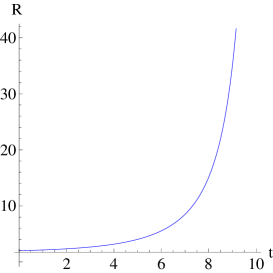
Figure 1: The plot of $R(t)$ of $F(R,G)=1+2G\ln{G}$ model at classical level.

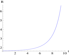
Figure 2: The plot of $R(t)$ of $F(R,G)=1+2G\ln{G}$ model, with $N=1$.

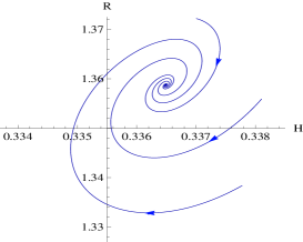
Figure 3: The spiral paths in $R-H$ plane of $F(R,G)=1+2G\ln{G}$, with $N=5$, at quantum level.

Other interesting cases also exist. For $a_{1}a_{2}<0$, where classically there is no critical point, quantum effects can induce a stable attractor. Fig.4 shows the phase-space of $F(R,G)=1-\frac{1}{8}G\ln{G}$ model with $N=1$ background. As it is seen, the point $(R_{c},H_{c})=\left(6.93,0.76\right)$ is a stable attractor of this model, which has no analogous at classical level.

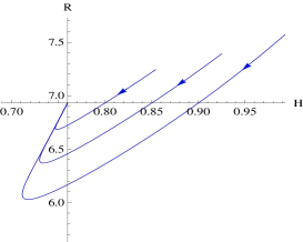
Figure 4: The paths of $F(R,G)=1-\frac{1}{8}\ln{G}$, with $N=1$, at quantum level.

3.2 $F(R,G)=a_{1}+a_{2}R+a_{3}R^{2}$ models

In the previous example, there is one critical point in each classical and quantum mechanical levels, and at $b^{\prime}\rightarrow 0$, i.e. $\hbar\rightarrow 0$, limit, $R_{c}^{\phantom{c}\rm{quant.}}\rightarrow R_{c}^{\phantom{c}\rm{class.}}$. Now we consider the class of models in which the number of classical and quantum mechanical critical points are not the same, and more, at $b^{\prime}\rightarrow 0$ limit, some of the quantum attractors do not lead to classical ones.

Consider the following $f(R)$ gravity model

$$f(R)=a_{1}+a_{2}R+a_{3}R^{2}\,.$$ (45)

The only classical critical point is found by eq.(30), with $b^{\prime}=0$, as following

$$R_{c}^{\phantom{c}\rm{class.}}=-\frac{2a_{1}}{a_{2}}\,.$$ (46)

The condition of stability of this solution, using eq.(38), is

$$\eta=\frac{a_{2}}{6a_{3}}>0\,.$$ (47)

So to have a positive curvature attractor, $a_{1}a_{2}$ must be negative, and for its stability, $a_{2}a_{3}$ must be positive. Note that because of eq.(31), the negative values of $R_{c}$ are not acceptable, since they lead to imaginary Hubble constants, which are not physical.

After adding the quantum correction terms, the action (45) has two quantum critical points. Using (30), one finds

$$\begin{split}&R_{c1}^{\phantom{c1}\rm{quant.}}=\frac{-6a_{2}-\sqrt{{(6a_{2})}^{2}-24a_{1}b^{\prime}}}{b^{\prime}}\>,\\ &R_{c2}^{\phantom{c2}\rm{quant.}}=\frac{-6a_{2}+\sqrt{{(6a_{2})}^{2}-24a_{1}b^{\prime}}}{b^{\prime}}\>,\end{split}$$ (48)

and their corresponding $\delta$s, which determine the stability behavior of these points, are

$${\delta}_{1}\,=\,-\,{\delta}_{2}=\,\frac{2\sqrt{{(6a_{2})}^{2}-24a_{1}b^{\prime}}}{12a_{3}-(\frac{2}{3}b+b^{\prime\prime})}\,.$$ (49)

Let us first study the $b^{\prime}\rightarrow 0$ limit of curvatures in eq.(LABEL:47), which their values depend on the sign of $a_{2}$:

$$R_{c1}^{\phantom{c1}\rm{quant.}}\longrightarrow-\frac{12a_{2}}{b^{\prime}}\hskip 8.61108pt,\hskip 8.61108ptR_{c2}^{\phantom{c1}\rm{quant.}}\longrightarrow-\frac{2a_{1}}{a_{2}}\,=R_{c}^{\phantom{c}\rm{class.}}\hskip 8.61108pt,\hskip 8.61108pt\text{for}\hskip 8.61108pta_{2}>0$$ (50)

and

$$R_{c1}^{\phantom{c1}\rm{quant.}}\longrightarrow-\frac{2a_{1}}{a_{2}}=R_{c}^{\phantom{c}\rm{class.}}\hskip 8.61108pt,\hskip 8.61108ptR_{c2}^{\phantom{c2}\rm{quant.}}\longrightarrow-\frac{12a_{2}}{b^{\prime}}\,\hskip 8.61108pt,\hskip 8.61108pt\text{for}\hskip 8.61108pta_{2}<0.$$ (51)

Now we encounter a new situation, one of the quantum curvatures goes to classical value, and the other one diverges.

This behavior is the characteristic of ”singular perturbation theory”. Mathematicians divide the perturbation theory to two categories, ”regular” and ”singular”. In regular perturbation problem, the solution of the perturbed equation

$$f_{1}(x)+\varepsilon f_{2}(x)=0$$ (52)

is

$$x({\varepsilon})=\sum_{n=0}^{\infty}\,a_{n}{\varepsilon}^{n}$$ (53)

where $a_{0}$, i.e. the zero-order solution, is the solution of the unperturbed equation:

$$f_{1}(a_{0})=0\>.$$ (54)

This is the usual behavior that we almost always encounter in physics. But in some perturbation problems, the situation is different. In singular perturbation problem, these two solutions, i.e. the ”zero-order solution” and the solution of ”unperturbed problem”, do not coincide. In fact, the zero-order solution may depend on $\varepsilon$ and may exist only for nonzero $\varepsilon$. This situation occurs whenever the power of the perturbation terms are greater than the unperturbed terms [20]. Consider, for example, the following algebraic equation:

$$\varepsilon x^{2}+x-1=0.$$ (55)

Their solution are

$$x=\frac{1}{2{\varepsilon}}\left(-1\pm\sqrt{1+4\varepsilon}\>\right)\hskip 8.61108pt\Rightarrow\begin{cases}x_{1}=1-{\varepsilon}+2{\varepsilon}^{2}+\cdots\\ x_{2}=-{1}/{\varepsilon}-1+{\varepsilon}+\cdots\end{cases}$$ (56)

At $\varepsilon\rightarrow 0$ limit, $x_{1}\rightarrow 1$, which is the solution of the unperturbed equation $x-1=0$, while $x_{2}$, which diverges at $\varepsilon\rightarrow 0$, has no unperturbed analogous.

This highly dependence of a problem to the perturbation is frequently encountered in chaotic dynamical systems. The appearance of this kind of solutions shows that one can not discard the perturbative terms, i.e. it can not be ignored, sets to zero, in the equations and therefore in the solutions.

For the example in hand, i.e. the Lagrangian (45), the critical point equation (30) becomes

$$-a_{1}-\frac{1}{2}a_{2}R=\frac{b^{\prime}}{24}R^{2},$$ (57)

which is very similar to eq.(55). So it is natural we encounter the singular perturbation problem, with its mentioned behaviors. In this problem, one classical solution, increases to two quantum mechanical ones, which one of them, depending on the sign of $a_{2}$, goes to classical solution, and the other one blows up. This shows that one can not ignore the quantum correction terms and they must be always added to classical equations of motion. The classical attractor can be stable or not, depending on the sign of $a_{2}a_{3}$ , see eq.(47), but in quantum case, one of the solutions is always stable and the other is unstable, see eq.(49).

We may have, depend on the parameters, one positive $R_{c}^{\phantom{c}\rm{class.}}$ and one positive $R_{c}^{\phantom{c}\rm{quant.}}$, no positive $R_{c}^{\phantom{c}\rm{class.}}$ and one positive $R_{c}^{\phantom{c}\rm{quant.}}$, or one positive $R_{c}^{\phantom{c}\rm{class.}}$ and two positive $R_{c}^{\phantom{c}\rm{quant.}}$. As a specific example for the latter case, we consider the following action

$$F(R)=-1+R-R^{2}$$ (58)

in which we again write in $c^{-1}=360{(4\pi)}^{2}$ unit. Using eqs.(46)-(49), one finds $R_{c}^{\phantom{c}\rm{class.}}=2$ with $\eta=-1/6$, $R_{c1}^{\phantom{c}\rm{quant.}}=6+\sqrt{12}$ with $\delta_{1}=-\sqrt{12}/7$, and $R_{c2}^{\phantom{c1}\rm{quant.}}=6-\sqrt{12}$ with $\delta_{2}=\sqrt{12}/7$. So $R_{c}^{\phantom{c}\rm{class.}}$ and $R_{c2}^{\phantom{c1}\rm{quant.}}$ are unstable critical points and tend together at $b^{\prime}\rightarrow 0$ limit, while $R_{c1}^{\phantom{c1}\rm{quant.}}$ is a stable attractor which blows up at this limit, see eq.(50). We have chosen $N=1$, and other $N_{i}$’s equal to zero. Fig.5 shows the behavior of $R(t)$ in classical regime, which verifies the unstability nature of $R_{c}^{\phantom{c}\rm{class.}}$, and Fig.6 shows that $R_{c1}^{\phantom{c1}\rm{quant.}}$ is a stable attractor.

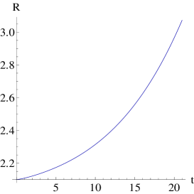
Figure 5: The plot of $R(t)$ of $F(R)=-1+R-R^{2}$ model at classical level.

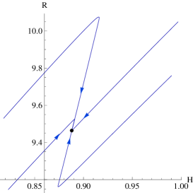
Figure 6: The quantum attractor of $F(R)=-1+R-R^{2}$ model, when $N=1$. The stable attractor $R_{c1}=6+\sqrt{12}$ blows up at $b^{\prime}\rightarrow 0$ limit.

3.3 $F(R,G)=a_{1}+a_{2}R+a_{3}R^{2}-a_{4}R^{2}\ln{R}$ models

As other interesting example, we consider the following $f(R)$ action:

$$f(R)=a_{1}+a_{2}R+a_{3}R^{2}-a_{4}R^{2}\ln{R}.$$ (59)

This model has two classical and two quantum-mechanical critical points, with coordinates

$$\begin{split}&R_{c1}^{\phantom{c1}\rm{class.}}=\frac{-a_{2}-\sqrt{{(a_{2})}^{2}-8a_{1}a_{4}}}{2a_{4}}\,,\\ &R_{c2}^{\phantom{c2}\rm{class.}}=\frac{-a_{2}+\sqrt{{(a_{2})}^{2}-8a_{1}a_{4}}}{2a_{4}}\,,\end{split}$$ (60)

and

$$\begin{split}&R_{c1}^{\phantom{c1}\rm{quant.}}=\frac{-a_{2}-\sqrt{{(a_{2})}^{2}-8a_{1}(a_{4}+b^{\prime}/12)}}{2a_{4}+{b^{\prime}}/{6}}\,,\\ &R_{c2}^{\phantom{c2}\rm{quant.}}=\frac{-a_{2}+\sqrt{{(a_{2})}^{2}-8a_{1}(a_{4}+b^{\prime}/12)}}{2a_{4}+{b^{\prime}}/{6}}\,,\end{split}$$ (61)

respectively. As $b^{\prime}$ tends to zero, irrespective of other parameters, it is clear from eqs.(LABEL:59) and (LABEL:60) that

$$R_{ci}^{\phantom{ci}\rm{quant.}}\hskip 4.30554pt\xrightarrow{\hskip 8.61108ptb^{\prime}\rightarrow 0\hskip 8.61108pt}\hskip 4.30554ptR_{ci}^{\phantom{ci}\rm{class.}}\hskip 12.91663pt,\>i=1,2\,.$$ (62)

However, this occurs whenever both classical and quantum critical curvatures, separately for each $i$ in eq.(62), belong to the same region, i.e. positive or negative curvatures. But if they are placed in different regions, e.g. $R_{c1}^{\phantom{c1}\rm{class.}}<0$ and $R_{c1}^{\phantom{c1}\rm{quant.}}>0$, we encounter a new problem. As a specific example, if we demand

$$R_{c1}^{\phantom{c1}\rm{class.}}<0\hskip 12.91663pt,\hskip 12.91663ptR_{c2}^{\phantom{c2}\rm{class.}}>0\hskip 12.91663pt,\hskip 12.91663ptR_{c1}^{\phantom{c1}\rm{quant.}}>0\hskip 12.91663pt,\hskip 12.91663ptR_{c2}^{\phantom{c2}\rm{quant.}}>0,$$ (63)

then the parameters must satisfy

$$b^{\prime}<0\hskip 17.22217pt,\hskip 17.22217pta_{2}>0\hskip 17.22217pt,\hskip 12.91663pt0<a_{4}<-\frac{b^{\prime}}{12}\hskip 12.91663pt,\hskip 12.91663pt\frac{3{a_{2}}^{2}}{24a_{4}+2b^{\prime}}\leq a_{1}<0.$$ (64)

Because of the condition $0<a_{4}<-{b^{\prime}}/{12}$, at $b^{\prime}\rightarrow 0$ limit, the parameter $a_{4}$ must also goes to zero. So the denominators of $R_{c1}^{\phantom{c1}\rm{class.}}$ and $R_{c1}^{\phantom{c1}\rm{quant.}}$ both go to zero, with different signs, while their numerators remain finite. Therefore

$$R_{c1}^{\phantom{c1}\rm{class.}}\hskip 5.69046pt \xrightarrow{\hskip 8.61108ptb^{\prime}\rightarrow 0\hskip 8.61108pt}\hskip 8.61108pt-\infty$$

$$R_{c1}^{\phantom{c1}\rm{quant.}}\hskip 2.84544pt \xrightarrow{\hskip 8.61108ptb^{\prime}\rightarrow 0\hskip 8.61108pt}\hskip 8.61108pt+\infty$$ (65)

This is another interesting behaviors of quantum $F(R,G)$ gravity models. The quantum effects increase the number of positive attractors, but the excess attractor blows up at $\hbar\rightarrow 0$ limit and does not approach to their corresponding classical solution. As an explicit example belongs to this category, we consider the following Lagrangian

$$f(R)=-1+2R+\frac{5}{6}R^{2}-\frac{1}{6}R^{2}\ln{R}\;,$$ (66)

and choose $N=3$ and other $N_{i}$’s are zero, so that $b^{\prime}=-3$. The critical points then become

$$\left(R_{c1}^{\phantom{c1}\rm{class.}},R_{c2}^{\phantom{c2}\rm{class.}}\right)\hskip 4.26773pt =\left(\,-3(2+4/\sqrt{3})\,,\,3(-2+4/\sqrt{3})\,\right),$$

$$\left(R_{c1}^{\phantom{c1}\rm{quant.}},R_{c2}^{\phantom{c2}\rm{quant.}}\right) =\left(\,2(6+\sqrt{30})\,,\,2(6-\sqrt{30})\,\right).$$ (67)

So we have one acceptable (positive) classical and two quantum mechanical critical points. All the critical points are stable attractors. $R_{c2}^{\phantom{c2}\rm{quant.}}$ tends to $R_{c2}^{\phantom{c2}\rm{class.}}$ at $b^{\prime}\rightarrow 0$, while $R_{c1}^{\phantom{c2}\rm{quant.}}$ has no classical analogous. Figs.7 and 8 show the behaviors of the stable attractors of this model at classical and quantum regimes, respectively.

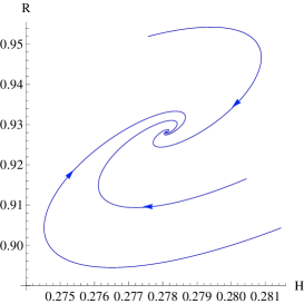
Figure 7: The classical critical point of $f(R)=-1+2R+\frac{5}{6}R^{2}-\frac{1}{6}R^{2}\ln{R}$ model.

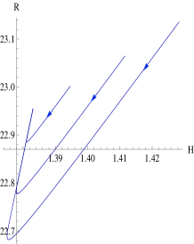
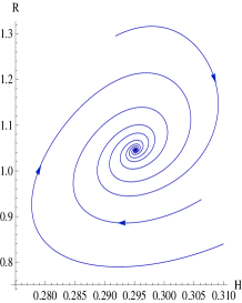
Figure 8: The quantum attractors of $f(R)=-1+2R+\frac{5}{6}R^{2}-\frac{1}{6}R^{2}\ln{R}$ model, when $N=3$.

The other interesting case of the Lagrangian (59), is one in which the classical curvatures become degenerate. This occurs when $(a_{2})^{2}=8a_{1}a_{4}$. In this case, one has

$$R_{c1}^{\phantom{c1}\rm{class.}}=R_{c2}^{\phantom{c2}\rm{class.}}=R_{\rm{class.}}=-\frac{a_{2}}{2a_{4}}\;,$$ (68)

and

$$R_{c1}^{\phantom{c1}\rm{quant.}}=\frac{R_{\rm{class.}}}{1-\sqrt{-\frac{b^{\prime}}{12a_{4}}}}\hskip 8.61108pt,\hskip 8.61108ptR_{c2}^{\phantom{c2}\rm{quant.}}=\frac{R_{\rm{class.}}}{1+\sqrt{-\frac{b^{\prime}}{12a_{4}}}}\>.$$ (69)

This phenomenon, in mathematics, is known as ”bifurcation”. In dynamical systems, if the problem depends on one (or more) parameter(s), and by continuous varying the parameter(s), two of the critical points collide each other, it is said there is a local bifurcation. In our problem, $b^{\prime}$ plays the role of the dynamical parameter. For $b^{\prime}\neq 0$, we have two attractors (69). By decreasing $b^{\prime}$ and reaching $b^{\prime}=0$, they collide and a single classical attractor (68) is produced.

Another characteristic of this degenerate solution is its $\eta$-value. To study the stability behaviors of $R_{\rm{class.}}$, one must calculate $\eta$ in eq.(38). For $f(R)$ in eq.(59), $\eta$ becomes, using eq.(31),

$$\eta=\frac{f_{R}}{3f_{RR}}-\frac{R}{3}=\frac{a_{2}+2a_{4}R}{3(2a_{3}-3a_{4}-2a_{4}\ln{R})}|_{R=R_{c}}$$ (70)

So for $R_{\rm{class.}}$ in eq.(68), one finds $\eta|_{R=R_{\rm{class.}}=0}$. This means that in this case, the eigenvalues of matrix $M$ are $\lambda_{1}=0$, $\lambda_{2}=-3H$ (see eq.(36) for classical case, in which $S+24H^{2}$ must be replaced by $-6\eta$). The appearance of zero eigenvalues in dynamical systems is an important point, which one of its consequences is that we can not predict the stability behavior of the attractors. In this case, the first order variation, which results in the stability matrix (33), is not adequate and one must consider the higher order approximations. This subject, for $F(R,G)$ gravity models, has been discussed in [14].

As an explicit example of the bifurcation point, we consider the following example:

$$f(R)=2-4R+2R^{2}-R^{2}\ln{R}$$ (71)

and $N=1$. Then $R_{\rm{class.}}=2$ and $R^{\rm{quant.}}_{\pm}=({24\pm 2\sqrt{12}})/{11}$. $R_{\rm{class.}}$ and $R^{\rm{quant.}}_{+}$ are unstable attractors, while $R^{\rm{quant.}}_{-}$ is a stable attractor, see Fig.9.

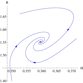
Figure 9: The quantum critical point $R^{\rm{quant.}}_{-}$ of $f(R)=2-4R+2R^{2}-R^{2}\ln{R}$ model with $N=1$.

As pointed out earlier, because of the degenerate nature of the classical attractors of this example, one can not easily determine the stability behavior of these critical points. In fact, if one follows the method described in [14], it can be shown that the next to leading order variation of Lagrangian (71), near $R_{\rm{class.}}=2$, is

$$\dot{\mathcal{U}}=6.9\,{\mathcal{U}}^{2}+\cdots,$$ (72)

where the positive coefficient of ${\mathcal{U}}^{2}$-term, proves the unstability of classical attractors near $R_{\rm{class.}}=2$.

4 The matter field’s contributions to attractors

In this section we want to study the contribution of matter fields to the structure of the phase-space, and investigate whether our results in previous sections are changed.

By considering ${\rho}_{m}$, the autonomous system of equations then consists of three equations, i.e. eqs.(27), (28) and eq.(14), and therefore the phase-space becomes 3-dimensional, i.e. $(R,H,{\rho}_{m})$. It must be noted that the variable $p_{m}$ in eq.(14) can be expressed, by using the equation of state of matter $p_{m}=f({\rho}_{m})$, in terms of ${\rho}_{m}$, so it is not an independent dynamical variable.

We restrict ourselves to barotropic fluid in which

$$p_{m}={\omega}_{m}{\rho}_{m}\>,$$ (73)

and ${\omega}_{m}$ is a constant. For example for dust, ${\omega}_{d}=0$, and for radiation, ${\omega}_{r}={1}/{3}$. In this case, the third autonomous differential equation becomes

$$\frac{d\rho_{m}}{dt}=-3H(1+{\omega}_{m}){\rho}_{m}\>.$$ (74)

One can write the new system of autonomous equations as:

$$\dot{H}=f_{1}(R,H,{\rho}_{m})\hskip 8.61108pt,\hskip 8.61108pt\dot{R}=f_{2}(R,H,{\rho}_{m})\hskip 8.61108pt,\hskip 8.61108pt{\dot{\rho}}_{m}=f_{3}(R,H,{\rho}_{m})\>.$$ (75)

The critical points are found by setting $\dot{H}=\dot{R}={\dot{\rho}}_{m}=0$. In this way, the critical point equations become the same as previous ones, i.e. eqs.(30) and (31), and the following extra relation:

$${\rho}_{mc}=0.$$ (76)

So the presence of the matter fields does not affect the position of the attractors, which comes from eqs.(30) and (31).

The stability matrix $M$ now becomes a $3\times 3$ matrix, as follows

$$M=\left(\begin{array}[]{ccc}-4H&1/6&0\\ S&H&B\\ 0&0&-3(1+{\omega}_{m})H\end{array}\right)_{R=R_{c},H=H_{c},{\rho}_{m}={\rho}_{mc}}\>,$$ (77)

in which

$$B=\frac{1}{6H(F_{RR}+8H^{2}F_{RG}+16H^{4}F_{GG})-(\frac{2}{3}b+b^{\prime\prime})H}\bigg{|}_{R=R_{c},H=H_{c}}\>.$$ (78)

The eigenvalues are: ${\lambda}_{1}$ and ${\lambda}_{2}$ in eq.(36), and

$${\lambda}_{3}=-3(1+{\omega}_{m})H_{c}\>.$$ (79)

So, as long as

$${\omega}_{m}>-1\,,$$ (80)

the eigenvalue ${\lambda}_{3}$ is negative and the stability situation is completely determined by eq.(37), or (38). In this way we obtain an important result: For barotropic fluids with ${\omega}_{m}>-1$, the structure of the phase-space is not changed. Note that the condition (80) satisfies by all ordinary, i.e. baryonic, matters.

The next point that we must consider is that the Lagrangian (15) has two kinds of effects in our problem. One of its role is its quantum contribution to the $F(R,G)$ gravity, which we have considered it by adding its $p_{A}$ and ${\rho}_{A}$ to the Friedmann equations. The second role of (15) is its classical contribution to our problem, which we have not yet considered it. To do so, one must consider the Friedmann equations of combined actions (7) and (15), i.e.

$$S=\int d^{4}x\sqrt{-g}{}\hskip 4.30554pt\left[F(R,G)+{\cal L}_{m}+\frac{1}{2}\left(-\xi R\phi^{2}-(\nabla\phi)^{2}\right)\right].$$ (81)

The other way is to consider the effects of extra action (15), by its energy density and pressure, i.e. ${\rho}_{\phi}$ and $p_{\phi}$, as the source terms for Friedmann equations (27) and (28). This can be done by considering the Friedmann equations of the scalar-tensor model (15) in the background of ordinary Einstein model, i.e.

$$S=\frac{1}{2}\int d^{4}x\sqrt{-g}{}\hskip 4.30554pt\left[R-\xi R\phi^{2}-(\nabla\phi)^{2}\right]\;,$$ (82)

which are [7]

$$3H^{2}\,=\,{\rho}_{\phi}\,=\,3\xi H^{2}{\phi}^{2}+\frac{1}{2}{\dot{\phi}}^{2}+6H\xi\phi{\dot{\phi}}\>,$$ (83)

$$-2\dot{H}\,=\,{\rho}_{\phi}+p_{\phi}\,=\,-2\xi\dot{H}{\phi}^{2}+2\xi H\phi\dot{\phi}-2\xi\phi\ddot{\phi}+(1-2\xi){\dot{\phi}}^{2}\>,$$ (84)

and

$$\ddot{\phi}+3H\dot{\phi}+\xi\phi(6\dot{H}+12H^{2})\,=\,0\>.$$ (85)

${\rho}_{\phi}$ is therefore given by eq.(83). $p_{\phi}$ can be found by subtracting (83) from (84), using (85), which results in

$$p_{\phi}=\left[2\xi(6\xi-1)\dot{H}+3\xi(8\xi-1)H^{2}\right]{\phi}^{2}+2\xi H\phi\dot{\phi}+(\frac{1}{2}-2\xi){\dot{\phi}}^{2}\>.$$ (86)

Then the trace of energy-momentum tensor, $T_{\phi}$, becomes

$$T_{\phi}=-{\rho}_{\phi}+3p_{\phi}=(1-6\xi){\dot{\phi}}^{2}+6\xi(6\xi-1)(\dot{H}+2H^{2}){\phi}^{2}.$$ (87)

This is a complicated expression which becomes very simple at $\xi={1}/{6}$. In fact

$$T_{\phi}(\xi=\frac{1}{6})\,=\,0\>.$$ (88)

This important equation has root in the conformal invariance of the action (15) at $\xi={1}/{6}$, as pointed out after eq.(15).

Because of eq.(88), we have

$$-{\rho}_{\phi}+3p_{\phi}\,=\,0\hskip 8.61108pt\Rightarrow\hskip 8.61108ptp_{\phi}\,=\,\frac{1}{3}{\rho}_{\phi}\;.$$ (89)

So one can add the classical contribution of action (15) to Friedmann equations by considering it as a barotropic fluid with ${\omega}_{\phi}={1}/{3}$! But we know that adding any barotropic fluid with $\omega>-1$ does not change the structure of phase-space, so this is also true for Lagrangian (15). This completes our proof.

5 Conclusion

In this paper we study the contribution of quantum phenomena on the structure of $R-H$ phase-space of $F(R,G)$ gravity models. It is shown that, both the location of de-sitter attractors and their stability properties, can change because of quantum corrections. These corrections are not, in general, from the type of small, and therefore ignorable, corrections, instead the topology of attractors may change. For the case where there is no attractor, it may produce some attractors, an example of it is discussed in section 3.1. In some cases, it increases the number of the attractors and their stability characteristics, with an important property: The increased attractors do not converge to classical ones at $\hbar\rightarrow 0$ limit, and more, their locations blow up. A fact which is known in the context of ”singular perturbation”. An example of this kind of behaviors is given in section 3.2. Also it is possible that the quantum contributions change the attractors, such that not only they do not converge to classical locations, but also the quantum and classical attractors go more distant from each other at $\hbar\rightarrow 0$ limit.

It is also shown that the barotropic perfect fluids with $\omega>-1$, do not change our results. Interestingly, the coupled-quintessence Lagrangian, which is responsible for producing the quantum terms, is from this type.

Besides the attractors studied in this paper, there are two other classes of attractors in $F(R,G)$ gravity models [14]. One of them is the singularities of $F(R,G)$ Lagrangian, which is always lead to the stable attractors, and the other class is one known as critical curve. The curve $R=12H^{2}$ is the location of infinite number of the stable attractors for the models whose Lagrangians satisfy eq.(30) (with $b^{\prime}=0$). That is, eq.(30) (with $b^{\prime}=0$) satisfies for all $R$ and $H$s. $F(R,G)=R^{2}g(G/R^{2}),F(R,G)=\alpha G+\beta R^{2},F(R,G)=R-6G/R,\cdots$, are examples of these Lagrangians [14]. Now it can be easily shown that the, so called, singular attractors do not change because of the quantum terms ${\rho}_{A}$ and $p_{A}$, but the critical curve $R=12H^{2}$, reduced to a single point. The reason is easy. If $F(R,G)$ satisfies

$$\frac{1}{2}RF_{R}+GF_{G}-F=0$$ (90)

for all $R$, then for these actions, the equation of critical point (30) becomes

$$0=6b^{\prime}H^{4}=\frac{1}{24}b^{\prime}R^{2}\>,$$ (91)

which has a unique solution $R_{c}=0$. So the quantum effects reduce the infinite number of stable attractor to an attractor at $R_{c}=0$.

Of course, the critical curve $R=12H^{2}$ still exists in our case, but for $F(R,G)$s which satisfy

$$\frac{1}{2}RF_{R}+GF_{G}-F=\frac{1}{24}b^{\prime}R^{2}$$ (92)

for all $R$ and $H$s. For these functions, since eq.(30) satisfies by $F(R,G)$, this equation does not impose any constraint on $R$ and $H$, and eq.(31) is the only equation which specifies the critical points. So $R=12H^{2}$ becomes the critical curve of these models. An example of these kinds of models is

$$f(R)=(C+\frac{b^{\prime}}{12}\ln{R})R^{2}\,,$$ (93)

which satisfies eq.(92). At $b^{\prime}\rightarrow 0$ limit, it gives $f(R)=R^{2}$, which is stated before (the $F(R,G)=\alpha G+\beta R^{2}$ model, with $\alpha=0$).

Acknowledgement: This work was partially supported by the ”center of excellence in structure of matter” of the Department of Physics of the University of Tehran, and also a research grant from the University of Tehran.

References

- [1] S. Perlmutter et al., Astrophys. J. 517 (1999) 565; A. G. Riess et al., Astron. J. 116 (1998) 1009; A. G. Riess et al., Astron. J. 117 (1999) 707; R. A. Knop et al., Astrophys. J. 598 (2003) 102; M. Tegmark et al., Phys. Rev. D 69 (2004) 103501; P. Astier et al., Astron. Astroph. 477 (2005) 31; D. N. Spergel et al., Astrophys. J. Suppl. 170 (2007) 377.
- [2] S. Weinberg, Rev. Mod. Phys. 61 (1989) 1.
- [3] C. Wetterich, Nucl. Phys. B 302 (1988) 668; S. M. Carroll, Phys. Rev. Lett. 81 (1998) 3067; H. Mohseni Sadjadi and M. Alimohammadi, Phys. Rev. D 74 (2006) 043506; R. R. Caldwell, Phys. Lett. B 545 (2002) 23; J. M. Cline, S. Jeon and G. D. Moore, Phys. Rev. D 70 (2004) 043543; B. Feng, X. -L. Wang and X. -M. Zhang, Phys. Lett. B 607 (2005) 35; M. Alimohammadi, Gen. Relativ. Grav. 40 (2008) 107; H. Wei, R. G. Cai and D. F. Zeng, Class. Quant. Grav. 22 (2005) 3189; H. Wei and R. G. Cai, Phys. Rev. D 72 (2005) 123507; M. Alimohammadi and H. Mohseni Sadjadi, Phys. Rev. D 73 (2006) 083527.
- [4] T. Chiba, T. Okabe and M. Yamaguchi, Phys. Rev. D 62 (2000) 023511; C. Armendariz-Picon, V. Mukhanov and P. J. Steinhardt, Phys. Rev. D 63 (2001) 103510; A. Y. Kamenshchik, U. Moschella and V. Pasquier, Phys. Lett. B 511 (2001) 265; V. Sahni and A. A. Starobinsky, Int. J. Mod. Phys. D 9 (2000) 373; M. Li, Phys. Lett. B 603 (2004) 1; Q. Huang and M. Li, J. Cosmol. Astropart. Phys 08 (2004) 013; H. Mohseni Sadjadi and N. Vadood, J. Cosmol. Astropart. Phys 08 (2008) 036.
- [5] P. Jordan, Naturwissenschaften 26 (1938) 417; M. Fierz, Helv. Phys. Acta 29 (1956) 128; C. H. Brans and R. H. Dicke, Phys. Rev. 124 (1961) 925.
- [6] P. G. Bergmann, Int. J. Theor. Phys. 1 (1968) 25; K. Nordtvedt, Astrophys. J. 161 (1970) 1059; R. V. Wagoner, Phys. Rev. D 1 (1970) 3209; S. Tsujikawa, K. Uddin, S. Mizuno, R. Tavakol and J. Yokoyama, Phys. Rev. D 77 (2008) 103009.
- [7] M. Alimohammadi and H. Behnamian, Phys. Rev. D 80 (2009) 063008.
- [8] S. Nojiri and S. D. Odintsov, Int. J. Geom. Methods Mod. Phys. 4 (2007) 115; T. P. Sotiriou and V. Faraoni, arXiv:0805.1726
- [9] S. M. Carroll, A. De Felice, V. Duvvuri, D. A. Easson, M. Trodden and M. S. Turner, Phys. Rev. D 71 (2005) 063513; T. Chiba, J. Cosmol. Astropart. Phys 03 (2005) 008; G. Cognola and S. Zerbini, Int. J. Theor. Phys. 47 (2008) 3186.
- [10] A. Nunez and S. Solganik, Phys. Lett. B 608 (2005) 189.
- [11] G. Cognola, E. Elizalde, S. Nojiri, S. D. Odintsov, and S. Zerbini, Phys. Rev. D 73 (2006) 084007.
- [12] T. Koivisto and D. F. Mota, Phys. Lett. B 644 (2007) 104; Phys. Rev. D 75 (2007) 023518.
- [13] M. Alimohammadi and A. Ghalee, Phys. Rev. D 79 (2009) 063006.
- [14] M. Alimohammadi and A. Ghalee, Phys. Rev. D 80 (2009) 043006.
- [15] A. Starobinsky, Phys. Lett. B 91 (1980) 99.
- [16] S. Nojiri and S. D. Odintsov, Phys. Lett. B 562 (2003) 147; Phys. Rev. D 70 (2004) 103522.
- [17] M. Alimohammadi and L. Sadeghian, J. Cosmol. Astropart. Phys. 01 (2009) 035.
- [18] E. J. Copeland, A. R. Liddle and D. Wands, Phys. Rev. D 57 (1998) 4686; S. C. C. Ng, N. J. Nunes and F. Rosati, Phys. Rev. D 64 (2001) 083510; E. J. Copeland, M. R. Garousi, M. Sami and S. Tsujikawa, Phys. Rev. D 71, (2005) 043003; V. Faraoni, S. Nadeau, Phys. Rev. D 72 (2005) 124005; V. Faraoni, Phys. Rev. D 72 (2005) 061501; L. Amendola, R. Gannouji, D. Polarski and S. Tsujikawa, Phys. Rev. D 75 (2007) 083504; S. -Y. Zhou, E. J. Copeland and P. M. Saffin, J. Cosmol. Astropart. Phys. 07 (2009) 009.
- [19] N. D. Birrell and P. C. W. Davies ”Quantum Fields in Curved Space” Cambridge University Press, 1986.
- [20] C. M. Bender and S. A. Orszag, ”Advanced Mathematical Methods for Scientists and Engineers”, McGraw-Hill, 1984; E. M. de Jager and Z. Furu, ”The Theory of Singular Perturbation”, Elsevier, 1996.