Random Convex Hulls and Extreme Value Statistics

Abstract

In this paper we study the statistical properties of convex hulls of $N$ random points in a plane chosen according to a given distribution. The points may be chosen independently or they may be correlated. After a non-exhaustive survey of the somewhat sporadic literature and diverse methods used in the random convex hull problem, we present a unifying approach, based on the notion of support function of a closed curve and the associated Cauchy’s formulae, that allows us to compute exactly the mean perimeter and the mean area enclosed by the convex polygon both in case of independent as well as correlated points. Our method demonstrates a beautiful link between the random convex hull problem and the subject of extreme value statistics. As an example of correlated points, we study here in detail the case when the points represent the vertices of $n$ independent random walks. In the continuum time limit this reduces to $n$ independent planar Brownian trajectories for which we compute exactly, for all $n$, the mean perimeter and the mean area of their global convex hull. Our results have relevant applications in ecology in estimating the home range of a herd of animals. Some of these results were announced recently in a short communication [Phys. Rev. Lett. 103, 140602 (2009)].

1 Introduction

Convex sets are defined by the property that the line segment joining any two points of the set is itself fully contained in the set. In the physical world, convex shapes are encountered in many instances, from convex elements that ensure acoustic diffusion in concert halls Ros , to crystallography, where the so-called Wulff construction leads, in the most general case, to a convex polyhedron whose facets correspond to crystal planes minimizing the surface energy Wu . Also, recent work in neuroscience indicates that the human brain seems better able to distinguish between two distinct shapes when these are both convex Neuro , which is particularly interesting since convexity properties are widely used in computer-aided image processing, in particular for pattern recognition AklTou . Such applications would be limited if they were restrained to intrinsically convex shapes; but it is not the case, since it is possible to ”approximate”, in some sense, a non-convex object by a convex one: pick, among all convex sets that can enclose a given object, the smallest one in terms of volume. This is called its convex hull, and comparing convex hulls can be a viable mean of comparing the shapes of complex patterns such as proteins and docking sites Pro . Convex hulls thus attract much interest, both for the algorithmic challenges set by their computation Grah ; JAl ; EdAl ; PHAl ; DevAL ; KSAl ; BSAl ; WAl ; Seidel ; Tou2 and for their applications Pro ; AklTou ; CHMedic ; CHIm ; Worton .

Random convex hulls are the convex hulls of a set of $N$ random points in a plane chosen according to some given distribution. The points may be chosen independently each from an identical distribution, e.g., from a uniform distribution over a disk. Alternatively, the points may actually be correlated, e.g., they may represent the vertices of a planar random walk of $N$ steps. For each realization of the set of points, one can construct the associated convex hull. Evidently, the convex hull will change from one realization of points to another. Naturally, all geometric characteristics of the convex hull, such as its perimeter, area, the number of vertices etc. also become random variables, changing their values from one realization of points to another. The main problem that we are concerned here is to compute the statistics of such random variables. For example, given the distribution of the points, what is the distribution of the perimeter or the area of the associated convex hull? It turns out that the computation of even the first moment, e.g., the mean perimeter or the mean area of the convex hull is a nontrivial problem.

This question has aroused much interest among mathematicians over the past 50 years or so, and has given rise to a substantial body of literature some of which will be surveyed in Section 2. The methods used in this body of work turn out to be diverse and sometimes specific to a given distribution of points. It is therefore important to find a unified approach that allows one to compute the mean perimeter and area, both in the case of independent points as well as when they are correlated such as in Brownian motion. The main purpose of this paper is to present such an approach. This approach is built on the works of Takács Ta , Eddy Ed and El Bachir El and the main idea is to use the statistical properties of a single object called the ‘support function’ which allows us, using the formulae known as Cauchy, Cauchy-Crofton or Cauchy-Barbier formulae Cau ; Cro ; BaE ; San ; Val ; AD , to compute the mean perimeter and the mean area of random convex hulls. This unified approach allows us to reproduce the existing results obtained by other diverse approaches, and in addition also provides new exact results, in particular for the mean perimeter and the mean area of $n$ independent planar Brownian motions (both for open and closed paths), a problem which has relevant applications in ecology in estimating the home range of a herd of animals. The latter results were recently anounced in a short Letter RFSMAC .

Our unified approach using Cauchy’s formulae also establishes an important link to the subject of extreme value statistics that deals with the study of the statistics of extremes in samples of random variables. In the random convex hull problem when the sample points are independent and identically distributed (i.i.d) in the plane, then the associated extreme value problem via Cauchy’s formulae is the classical example of extreme value statistics (EVS) of i.i.d random variables that is well studied, has found a lot of applications ranging from climatology to oceanography and has a long history EVSG1 ; EVSG2 ; Gne ; EVSC . For example, in the physics of disordered systems the EVS of i.i.d variables plays an important role in the celebrated random energy model Derrida ; BMM . In contrast, when the points are distributed in a correlated fashion, as in the case where they represent the vertices of a random walk, our approach requires the study of the distribution of the maximum of a set of correlated variables, a subject of much current interest in a wide range of problems (for a brief review see SMPK ) such as in fluctuating interfaces Burkhardt ; Gyorgi1 ; Gyorgi2 ; Roy ; ACSM1 ; SMAC ; GSSM ; Rambeau ; Gyorgi2 , in logarithmically correlated Gaussian random energy models for glass transition CPL ; FB1 ; Rosso1 , in the properties of ground state energy of directed polymers in a random media Johansson ; DS ; DDSM1 ; PLD1 ; SMPK2 ; Sire1 and the associated computer science problems on binary search trees SMPK1 ; SMPK3 ; BKM and the biological sequence matching problems Nechaev1 , in evolutionary dynamics and interacting particle systems KJ ; SMD ; BenaM ; SS ; Mallick , in loop-erased random walks AgDh , in queueing theory applications KM , in random jump processes and their applications CFFH ; CMM ; MZC , in branching random walks Mckean ; Bramson ; BDer , in condensation processes EM , in the statistics of records Krug ; MZ ; GL ; PLKW and excursions in nonequilibrium processes GMS ; Rosso ; Sire , in the density of near-extreme events SSSM ; SMR , and also in various applications of the random matrix theory TW ; DM1 ; DM2 ; BBP ; VMB ; Lak1 ; Lak2 ; SMCRF ; MV1 ; Nad . Here, our approach establishes yet another application of EVS, namely in the random planar convex hull problem.

The paper is organised as follows. In Section 2, we provide a non-exhaustive survey of the literature on random convex hulls. In Section 3, we introduce the notion of the ‘support function’ and the associated Cauchy formulae for the perimeter and the area of any closed convex curve. This section also establishes the explicit link to extreme value statistics. We show in Section 4 how to derive the exact mean perimeter and the mean area of the convex hull of $N$ independent points using our approach. Section 5 is fully devoted to the case when the points represent the vertices of a Brownian motion, a case where the points are thus correlated. Finally we conclude in Section 6 with some open questions. Some of the details are relegated to the Appendices.

2 A (non-exhaustive) review of results on random convex hulls

In this section we briefly review a certain number of results on the the convex hull of randomly chosen points. This review is of course far from exhaustive and we choose only those results that are more relevant to this work. They are presented in a chronogical order and at the end of the section we summarize in a table the results that are particularly relevant to the present work.

• In his book on random processes and Brownian motion (published in 1948) Lev , P. Lévy mentions, in a few paragraphs and mainly heuristically the question of the convex hull of planar Brownian motion: ”This contour [that of the convex hull of planar Brownian motion] consists, except for a null-measure set, in rectilinear parts.”

• More than ten years later, in 1959, J. Geffroy seems to be the first to publish results pertaining to the convex hull of a sample of random points drawn from a given distribution Ge1 , specifically $N$ points chosen in $\mathbb{R}^{2}$ according to a Gaussian normal distribution $f$. He shows that if one denotes

  • by $\partial C_{N}$ the boundary of the convex hull of the sample,

  • by $\Sigma_{N}$ the ellipsoid given by the equation $f(x,y)=\frac{1}{N}$,

  • by $\Delta_{N}$ the distance between $\partial C_{N}$ and $\Sigma_{N}$,

  • and by $\Lambda_{N}$ the largest possible radius of an open disk whose interior lies inside the convex hull but contains none of the sample points,

  then almost surely:

  $$\Delta_{N}\text{ and }\Lambda_{N}\mathop{\longrightarrow}_{N\rightarrow\infty}0$$ (1)

  In other words, the convex hull of the sample ”tends” to the ellipsoid given by $f(x,y)=\frac{1}{N}$. Geffroy generalizes this result to $\mathbb{R}^{d}$, $d\geq 1$, in 1961 Ge2 .

• In 1961 F. Spitzer and H. Widom study the perimeter $L_{N}$ of the convex hull of a random walk represented by sums of random complex numbers $S_{0}=0,\cdots,S_{k}=Z_{1}+Z_{2}+\cdots Z_{k},1\leq k\leq N$, where the $Z_{k}$ are i.i.d. random variables. By combining an identity discovered by M. Kác with a formula due to A.-L. Cauchy (which is used here for the first time in the context of random convex hulls), they derive an elegant formula for the expectationSW :

  $$\mathbb{E}(L_{N})=2\sum_{k=1}^{N}\frac{\mathbb{E}(|S_{k}|)}{k},$$ (2)

  The asymptotic behaviour of $\mathbb{E}(L_{N})$ is studied in two different cases:

  1. Writing $Z_{k}=X_{k}+iY_{k}$ and taking $\mathbb{E}(X_{k})=\mathbb{E}(Y_{k})=0$, $\mathbb{E}(X_{k}^{2})=a^{2}$, $\mathbb{E}(Y_{k}^{2})=b^{2}$, and $\mathbb{E}(X_{k}Y_{k})=\rho ab$, one has:

     $$\mathbb{E}(L_{N})\mathop{\sim}_{N\rightarrow\infty}4c\sqrt{N},$$ (3)

     where $c(a,b,\rho)$ does not depend on $N$.

  2. Taking $Z_{k}=X_{k}+i$ with $\mathbb{E}(X_{k})=\mu$ and $\mathbb{E}((X_{k}-\mu)^{2})=\sigma^{2}$, one has:

     $$\mathbb{E}(L_{N})\mathop{\sim}_{N\rightarrow\infty}2N\sqrt{1+\mu^{2}}+\frac{\sigma^{2}}{(1+\mu^{2})^{\frac{3}{2}}}\log N,$$ (4)

     which expresses the excess of $\mathbb{E}(L_{N})$ over its smallest possible value $2N\sqrt{1+\mu^{2}}$ .

• In the same year, and still for very general random walks viewed as a sum of $N$ vectors in the complex plane $S_{0}=0,\cdots,S_{k}=Z_{1}+Z_{2}+\cdots Z_{k},1\leq k\leq N$, G. Baxter Bax establishes three formulae involving respectively

  • the number $F_{N}$ of edges of the convex hull of the random walk,

  • the number $K_{N}$ of steps $Z_{k}$ from the walk which belong to the boundary of the convex hull,

  • the perimeter $L_{N}$ of the of the convex hull .

  In the latter case, Baxter’s formula coincides with Eq. (2), but Baxter’s derivation rests purely on combinatorial arguments and does not make use of Cauchy’s formula. Instead, it relies on counting the number of permutations of the random walk’s steps for which a given partial sum $S_{k}$ belongs to the boundary of the convex hull.
  His formulae are:

  $$\mathbb{E}(F_{N}) = 2\sum_{m=1}^{N}\frac{1}{m}\sim 2\log N$$ (5)

  $$\mathbb{E}(K_{N}) = 2$$ (6)

  $$\mathbb{E}(L_{N}) = 2\sum_{k=1}^{N}\frac{\mathbb{E}(|S_{k}|)}{k}.$$ (7)

• In 1963, appears the first RS of two seminal papers by A. Rényi and R. Sulanke dealing with the convex hull of $N$ independent, identically distributed random points $P_{i}$ ($i=1..N$) in dimension 2. Denoting by $F_{N}$ the number of edges of the convex hull, they consider the following cases:

  1. the $P_{i}$’s are distributed uniformly within a convex, $r$-sided polygon $K$:

     $$\mathbb{E}(F_{N})=\frac{2}{3}r(\log N+\gamma)+T(K)+\text{o}(1)$$ (8)

     where $\gamma$ is the Euler constant and $T(K)$ is a constant depending on $K$ only and which is maximal for regular $r$-sided polygons,

  2. the $P_{i}$’s are uniformly distributed within a convex set $K$ whose boundary is smooth:

     $$\mathbb{E}(F_{N})\mathop{\sim}_{N\rightarrow\infty}\alpha(K)N^{\frac{3}{2}},$$ (9)

     with $\alpha(K)$ a constant depending on $K$,

  3. the $P_{i}$’s have a Gaussian normal distribution throughout the plane:

     $$\mathbb{E}(F_{N})\mathop{\sim}_{N\rightarrow\infty}2\sqrt{2\pi\log N}$$ (10)

• The following year, 1964, the second of Rényi and Sulanke’s papers RS2 extend these results, focusing on the asymptotic behaviour ${N\rightarrow\infty}$ of the perimeter $L_{N}$ and area $A_{N}$ of the convex hull of $N$ points $P_{i}$ drawn uniformly and independently within a convex set $K$ of perimeter $L$ and area $A$:

  1. If $K$ has a smooth boundary:

     $$\mathbb{E}(L_{N}) = L-\mathcal{O}(N^{-\frac{2}{3}})$$ (11)

     $$\mathbb{E}(A_{N}) = A-\mathcal{O}(N^{-\frac{2}{3}})$$ (12)

  2. If $K$ is a square of side $a$:

     $$\mathbb{E}(L_{N}) = 4a-\mathcal{O}(N^{-\frac{1}{2}})$$ (13)

     $$\mathbb{E}(A_{N}) = a^{2}-\mathcal{O}(\frac{\log N}{N})$$ (14)

• In 1965, B. Efron Ef , taking cue from Rényi and Sulanke, establish equivalent formulae in dimension 3, together with the average number of vertices (faces in dimension 3), the average perimeter and the average area of the convex hull of $N$ points drawn independently from a Gaussian normal distribution in dimension 2 or 3, or from a uniform distribution inside a disk or sphere:

  1. For instance, for $N>3$ points in the plane, drawn independently from a Gaussian normal distribution, writing $\phi(x)=(2\pi)^{-\frac{1}{2}}\exp(-\frac{1}{2}x^{2})$ and $\Phi(x)=\int_{-\infty}^{x}\phi(y)\ dy$:

     $$\mathbb{E}(V_{N}) = 4\sqrt{\pi}\binom{N}{2}\int_{-\infty}^{\infty}\Phi^{N-2}(p)\phi^{2}(p)\ dp,$$ (15)

     $$\mathbb{E}(L_{N}) = 4\pi\binom{N}{2}\int_{-\infty}^{\infty}\Phi^{N-2}(p)\phi^{2}(p)\ dp,$$ (16)

     $$\mathbb{E}(A_{N}) = 3\pi\binom{N}{3}\int_{-\infty}^{\infty}\Phi^{N-3}(p)\phi^{3}(p)\ dp,$$ (17)

     where $V_{N}$, $L_{N}$ and $A_{N}$ stand respectively for the number of vertices, perimeter and area of the convex hull .

  2. In dimension 3, one has:

     $$\mathbb{E}(F_{N}) = 4\sqrt{3\pi}\binom{N}{3}\int_{-\infty}^{\infty}\Phi^{N-3}(p)\phi^{3}(p)\ dp,$$ (18)

     $$\mathbb{E}(E_{N}) = \frac{3}{2}\mathbb{E}(F_{N}),$$ (19)

     $$\mathbb{E}(V_{N}) = \frac{1}{2}\mathbb{E}(F_{N})+2,$$ (20)

     $$\mathbb{E}(L_{N}) = 24\sqrt{3\pi}\binom{N}{3}\int_{-\infty}^{\infty}\Phi^{N-3}(p)\phi^{3}(p)\ dp,$$ (21)

     $$\mathbb{E}(A_{N}) = 12\pi\binom{N}{3}\int_{-\infty}^{\infty}\Phi^{N-3}(p)\phi^{3}(p)\ dp,$$ (22)

     $F_{N}$ and $E_{N}$ standing respectively for the number of faces and the number of edges of the convex hull ($L_{N}$ is thus the sum of the lengths of the edges, and $A_{N}$ the sum of the surface areas of the faces, $V_{N}$ denotes again the number of vertices).

  He also computes the average volume of the convex hull of $N$ vectors drawn independently from a Gaussian normal distribution (with zero average and unit variance) in a space of dimension $d<N$:

  $$\mathbb{E}(\text{Vol}_{N})=\frac{2\pi^{\frac{1}{2}d}}{\Gamma(\frac{1}{2}d)}\left(\frac{d+1}{d}\right)\binom{N}{d+1}\int_{-\infty}^{\infty}\Phi^{N-d-1}(p)\phi^{d+1}(p)\ dp$$ (23)

  (for $N=d+1$, this expression needs to be multiplied by 2).

• In 1965 still, H. Raynaud communicates in the Comptes Rendus de l’Académie des Sciences Ray1 , his generalization to $\mathbb{R}^{d}$ of the formulae by Rényi-Sulanke and Efron pertaining to the number of vertices of the convex hull, either in the Gaussian normal case or in the uniform case. In the case of a Gaussian normal case, with zero mean and variance $a/2$, Raynaud computes the probability density of the convex hull of a sample and shows that, in the limit when the number of points $N$ in the sample becomes very large, this distribution converges to a uniform Poisson distribution on the sphere of radius $\sqrt{a\log N}$ centered at the origin.

• In 1970, H. Carnal Ca addresses the question of the convex hull of $N$ random points in the plane, drawn from a distribution which he assumes only to be circularly symmetric. He gives expressions for the asymptotic behaviour of the average number of edges, average perimeter and average area of the convex hull. In particular, he shows that the average number of edges, for certain distributions, goes to a constant (namely 4) when $N$ becomes very large.

• H. Raynaud publishes in 1970 a second paper Ray2 on the convex hull of $N$ independent points (in both the Gaussian normal case throughout the space or the uniform case within a sphere) in $\mathbb{R}^{d}$. He gives detailed accounts of the results he announced earlier Ray1 . He also gives expressions for the asymptotic behaviour of the number of faces $F^{(d)}_{N}$ (or edges if $d=2$) of the convex hull, and shows in particular that in the standard Gaussian normal case:

  $$\mathbb{E}(F^{(d)}_{N})\mathop{\sim}_{N\rightarrow\infty}\frac{2^{d}}{\sqrt{d}}\left(\pi\log N\right)^{\frac{1}{2}(d-1)}$$ (24)

  Note that for $d=2$, one recovers Rényi and Sulanke’s formula Eq.( 10). For $d=3$, one has $\mathbb{E}(F^{(3)}_{N})\sim\frac{8}{\sqrt{3}}\pi\log N$

• Ten years later, in 1980, W. Eddy Ed introduces the notion of support function into the field of random convex hulls. Considering, in the plane, $N$ points $P_{i}=(x_{i},y_{i})$ with a Gaussian normal distribution, he associates to each a random process defined by:

  $$B_{i}(\theta)=x_{i}\cos\theta+y_{i}\sin\theta,$$

  $\theta$ varying from $0$ to $2\pi$. Note that $B_{i}(\theta)$ is simply the projection of point $P_{i}$ on the line of direction $\theta$. He further defines the random process

  $$M(\theta)=\mathop{\sup}_{i}\{B_{i}(\theta)\},$$

  whose law is shown to be given by that of the pointwise maximum of the $N$ independent, identically distributed random processes $B_{i}(\theta)$ (cf BR ). Eddy then shows that the point distribution of the stochastic process $M(\theta)$ is given by Gumbel’s law, and he hints (without going further) to the fact that certain functionals of $M(\theta)$ give access to some geometrical properties of the convex hull of the sample:

  $$L_{N}=\int_{0}^{2\pi}M(\theta)d\theta$$ (25)

  for the perimeter; and:

  $$A_{N}=\frac{1}{2}\int_{0}^{2\pi}\left[M^{2}(\theta)-(M^{\prime}(\theta))^{2}\right]d\theta$$ (26)

  for the area, where $M^{\prime}(\theta)=\frac{dM}{d\theta}$. These functionals are what we refer to as Cauchy’s formulae.

• It is precisely the first of these formulae that L. TakácsTa suggests one should use to compute the expected perimeter length of the convex hull of planar Brownian motion, in his 1980 solution to a problem set by G. Letac in the American Mathematical Monthly in 1978 Le1 . Denoting by $L_{t}$ the perimeter of the convex hull of Brownian motion ${B(\tau),0\leq\tau\leq t}$ , Takács shows that:

  $$\mathbb{E}(L_{t})=\sqrt{8\pi t}.$$ (27)

  The calculation is performed using the support function of the trajectory, in the same way as Eddy Ed hinted at for independent points. Planar Brownian motion $B(\tau)$ is written as $(x(\tau),y(\tau))$, where $x$ and $y$ are standard one-dimensional Brownian motions. One then defines

  $$z_{\tau}(\theta)=x(\tau)\cos\theta+y(\tau)\sin\theta.$$

  This stochastic process $z_{\tau}(\theta)$ being nothing else but the projection of the planar motion on the line with direction $\theta$, it is itself, for a fixed $\theta$, an instance of standard Brownian motion. Hence, the $M(\theta)$ that appears in Cauchy’s formula (Eq. (25)) and which is defined as:

  $$M(\theta)=\mathop{\max}_{0\leq\tau\leq t}\{z_{\tau}(\theta)\},$$

  follows for a given $\theta$ the same law as the maximum of a standard one-dimensional Brownian motion. In particular, it is independent of $\theta$ and therefore one can write:

  $$\mathbb{E}(L_{t})=2\pi\ \mathbb{E}\left(M(0)\right),$$

  thus using the isotropy of the distribution of planar Brownian motion. Knowledge of the right-hand part of this equation then yields the desired result.

• In 1981, W. Eddy and J. Gale EG extend further the work started by W. Eddy Ed They point out the link between extreme-value statistics applied to $N$ 1-dimensional random variables and the distribution of the convex hull of multidimensional random variables. They consider sample distributions with spherical symmetry and distinguish between three classes according to the shape of the tails: exponential, algebraic (power-law) or truncated (e.g. distributed inside a sphere). Eddy and Gale then compute the asymptotic distribution of the associated stochastic process (the support function $M(\theta)$) when the number $N$ of points becomes very large. The three classes of initial sample distribution yield three types of distribution for the limit process, given by the Gumbel, Fréchet and Weibull laws, which are well known in the context of extreme-value statistics. Eddy and Gale also remark that the average number of vertices of the convex hull in the ”Fréchet” case (that is, for initial sample distributions with power-law tails) tends to a constant (as proved by Carnal Ca ).

• Following another route, N. Jewell and J. Romano establish the following year, in 1982, a correspondance between the random convex hull problem and a coverage problem, namely the covering of the unit circle with arcs whose positions and lengths follow a bivariate law JR . Thus, for arcs of length $\pi$:

  Prob (circle covered) $=$ Prob (conv. hull contains origin)

  and more generally, for arcs of lengths other than $\pi$:

  Prob (circle covered) $=$ Prob (conv. hull contains a given disk)

• In 1983, M. El Bachir, in his doctoral dissertation El , studies the convex hull $C(t)$ of planar Brownian motion $B(t)$. In particular, he gives a proof of P. Lévy’s assertion Lev that almost surely $C(t)$ has a smooth boundary. El Bachir also shows that $C(t)$ is a Markov process on the set of compact convex domains containing the origin $O$. Denoting by $\partial C(t)$ the boundary of $C(t)$, he establishes:

  1. $\mathrm{Prob}(B(t)\in\partial C(t))=\mathrm{Prob}(O\in\partial C(t))=0$

  2. $\{t:B(t)\in\partial C(t)\}$ has a null Lebesgue measure .

  El Bachir then computes explicitly, from Cauchy’s formulae, the expected perimeter length and surface area of the convex hull of planar Brownian motion. For the perimeter, he derives a general formula for motions with a drift $\mu$, of which the special case $\mu=0$ enables one to retrieve Takács’ $\sqrt{8\pi t}$. For the area, he obtains:

  $$\mathbb{E}(A_{t})=\frac{\pi t}{2}.$$ (28)

• Over the following decade, the study of the convex hull of a sample of independent, identically distributed random points has attracted much interest. C. Buchta B1 has obtained an exact formula giving the average area of the convex hull of $N$ points drawn uniformly inside a convex domain $K$, the existing formulae being so far mainly asymptotic. A few years later, F. Affentranger Aff has extended Buchta’s result to higher dimensions, via an induction relation. Many details and references can be found in the surveys of Buchta B2 , R. Schneider Sch , W. Weil and J. Wieacker WW .

• Another active route is the one open by Eddy Ed and Gale EG , whose works have been extended by H. Brozius and de Haan BH to non-rotationally-invariant distributions. Brozius et al Bro also study the convergence in law to Poisson point processes exhibited by the distributions of quantities such as the number of vertices of the convex hull of independent, identically distributed random points. The works of Davis et al. Davis and Aldous et al. Ald also follow this type of approach.

• Cranston et al. CHM resume the study of the convex hull $C(t)$ of planar Brownian motion and in particular of the continuity of its boundary $\partial C(t)$. They show that $\partial C(t)$ is almost surely $C^{1}$ and mention work by Shimura Shi1 ; Shi2 and K. Burdzy Bu showing that for all $\alpha\in(\frac{\pi}{2},\pi)$, there exist random times $\tau$ such that $C(\tau)$ has corners of opening $\alpha$. They also mention Le Gall LeG showing that the Hausdorff dimension of the set of times at which the Brownian motion visits a corner of $C(t)$ of opening $\alpha$ is almost surely equal to $1-\frac{\pi}{2\alpha}$. Finally, they also point to P. Lévy’s paper Lev2 and S. N. Evas’ Ev for details on the growth rate of $C(t)$, as well as to K. Burdzy and J. San Martin’s work KBSM on the curvature of $C(t)$ near the bottom-most point of the Brownian trajectory.

• In 1992, D. Khoshnevisan Kho elaborates upon Cranston et al.’s work by establishing an inequality that allows one to transpose, in some sense, the scaling properties of Brownian motion to its convex hull.

• In 1993, two papers concerned with the convex hull of correlated random points, specifically the vertices of a random walk, are published. G. Letac Le2 points out that Cauchy’s formula enables one to write the perimeter $L_{N}$ of the convex hull of any $N$-step random walk in terms of its support function $M_{N}(\theta)=\mathop{\max}_{0\leq i\leq N}\{x_{i}\cos\theta+y_{i}\sin\theta\}$:

  $$\mathbb{E}(L_{N})=\int_{0}^{2\pi}\ \mathbb{E}\left(M_{N}(\theta)\right)\ d\theta,$$ (29)

  which provides an alternative to Spitzer-Widom’s or Baxter’s methods to compute the perimeter of the convex hull of a random walk.
  

  It is precisely to the Spitzer-Widom-Baxter’s formula (Eq. (2)) that T. Snyder and J. Steele SnS return, using again purely combinatorial arguments to obtain the following generalizations :
  

  Let $F_{N}$ be the number of edges of the convex hull of a $N$-step planar random walk and let $e_{i}$ be the length of the $i$-th edge. If $f$ is a real-valued function and if we set $G_{N}=\sum_{i=1}^{F_{N}}f(e_{i})$, then:

  $$\mathbb{E}(G_{N})=2\sum_{k=1}^{N}\frac{\mathbb{E}\left(f\left(|S_{k}|\right)\right)}{k},$$ (30)

  where $S_{k}=Z_{1}+Z_{2}+\cdots Z_{k}$ is the position of the walk after $k$ steps.
  

  • Taking $f(x)=1$, one has $G_{N}=F_{N}$ (the number of edges of the convex hull) and one retrieves Baxter’s result

    $$\mathbb{E}(F_{N})=2\sum_{k=1}^{N}\frac{1}{k}\mathop{\sim}_{N\rightarrow\infty}2\log N.$$

  • Taking $f(x)=x$, one has $G_{N}=L_{N}$ and one retrieves Spitzer and Widom’s result without using Cauchy’s formula:

    $$\mathbb{E}(L_{N})=2\sum_{k=1}^{N}\frac{\mathbb{E}\left(|S_{k}|\right)}{k}.$$

  • Taking $f(x)=x^{2}$, $G_{N}$ is the sum of the squared edges lengths denoted by $L_{N}^{(2)}$, one obtains:

    $$\mathbb{E}\left(L_{N}^{(2)}\right)=2N(\sigma_{X}^{2}+\sigma_{Y}^{2}),$$

    $\sigma_{X}^{2}+\sigma_{Y}^{2}$ being the variance of an individual step.

  Snyder and Steele establish two other important results:

  1. An upper bound for the variance $\mathbb{E}\left(L_{N}^{2}\right)$ (not to be mistaken for $\mathbb{E}\left(L_{N}^{(2)}\right)$) of the perimeter of the convex hull of any $N$-step planar random walk:

     $$\mathbb{E}\left(L_{N}^{2}\right)\leq\frac{\pi^{2}}{2}N(\sigma_{X}^{2}+\sigma_{Y}^{2})$$ (31)

  2. A large deviation inequality for the perimeter of the convex hull of an $N$-step random walk:

     $$\mathrm{Prob}\left(|L_{N}-\mathbb{E}(L_{N})|\geq t\right)\leq 2e^{-\frac{t^{2}}{8\pi^{2}N}}$$ (32)

• In a paper published in 1996 Go , A. Goldman introduces a new point of view on the convex hull of planar Brownian bridge. He derives a set of new identities relating the spectral empiral function of a homogeneous Poisson process to certain functionals of the convex hull. More precisely:
  

  Let $D(R)$ be the open disk with radius $R$ and $D_{i}$ ($i=1..N_{R}$) the polygonal convex domains associated to a Poisson random measure and contained in $D(R)$. Let

  $$\phi_{i}(t)=\sum_{n=1}^{\infty}\exp(-t\lambda_{n,i})$$

  be the spectral function of the domain $D_{i}$ (the $\lambda_{n,i}$’s being the eigenvalues of the Laplacian for the Dirichlet problem on $D_{i}$). Finally, set:

  $$\phi_{R}(t)=\frac{1}{N_{R}}\sum_{i=1}^{N_{R}}\phi_{i}(t).$$

  Then:

  $\phi_{R}(t)$ almost surely has a finite limit $\Phi(t)$ (called the empirical spectral function) when $R$ goes to infinity, and:

  $$\Phi(t)=\frac{1}{4\pi^{2}t}\mathbb{E}\left(e^{-\sqrt{2t}L}\right)$$ (33)

  where $L$ stands for the perimeter of the convex hull of the unit-time planar Brownian bridge (a Brownian motion conditionned to return to its origin at time $t=1$).

  Goldman also computes the first moment of $L$ using Cauchy’s formula

  $$\mathbb{E}(L)=\sqrt{\frac{\pi^{3}}{2}}$$ (34)

  To obtain the second moment,

  $$\mathbb{E}(L^{2})=\frac{\pi^{2}}{3}\left(\pi\int_{0}^{\pi}\frac{\sin u}{u}\ du-1\right)$$ (35)

  Goldman brings it down to computing $\mathbb{E}(M(\theta)M(0))$, the two-point correlation function of the support function of the Brownian bridge,

  $$\mathbb{E}(M(\theta)M(0))=\frac{\sin\theta}{2}\left[\frac{\theta(2\pi-\theta)}{6(\pi-\theta)}+\mathrm{cotan}\theta\right]$$ (36)

  Goldman obtains this last result from the probability that the Brownian bridge $\mathcal{B}_{0,1}$ lies entirely inside a wedge $\xi$ of opening angle $\beta$:

  $$\mathrm{Prob}\left(\mathcal{B}_{0,1}\in\xi\right)=\frac{4\pi e^{-r^{2}}}{\beta}\sum_{k=1}^{\infty}\sin^{2}\left(\frac{k\pi\alpha}{\beta}\right)I_{\nu}(r^{2}),$$ (37)

  with $\nu=\frac{k\pi}{\beta}$, and, assuming that $O$ lies inside the wedge $\xi$, with $r$ the distance between $O$ and the apex $S$ of the wedge, and with $\alpha$ the angle between the line $OS$ and the closest edge of the wedge. ($I_{\nu}$ is the modified Bessel function of the first kind.)

• In a later paper Go2 , Goldman exploits further the link between Poissonian mosaics and the convex hull of planar Brownian bridges. He first shows that one can replace Brownian bridges by simple Brownian motion. He then recalls Kendall’s conjecture on Crofton’s cell (in a Poisson mosaic, this is the domain $D_{0}$ that contains the origin): when the area $V_{0}$ of this cell is large, its ”shape” would be ”close” to that of a disk. Goldman shows in this paper a result supporting this claim (in terms of eigenvalues of the Laplacian for the Dirichlet problem) and, thanks to the links he has established, deduces that the convex hull of planar Brownian motion, when it is ”small”, has an ”almost circular” shape. More precisely: if $C$ is the convex hull of a unit-time, planar Brownian motion $\mathcal{W}$, if $D(r)$ is the disk centered at the origin with radius $r\in(0,\infty)$ and if $M=\sup\{||W(s)||,0\leq s\leq 1\}$, then, for all $\epsilon\in(0,1)$:

  $$\limsup_{a\rightarrow 0}\mathrm{Prob}[D((1-\epsilon)a)\subset C\subset D(a)|M=a]=1$$ (38)

• In parallel, refined studies of the asymptotic distributions and limit laws of the number of vertices, perimeter or area of the convex hull of independent points drawn uniformly inside a convex domain $K$ continue, in particular with the work of P. Groeneboom Gro on the number of vertices (augmented by S. Finch and I. Hueter’s result FiH ), Hsing Hs on the area when $K$ is a disk, Cabo and Groeneboom CaGro for the area too but when $K$ is polygonal, Bräker and Hsing BHs for the joint law of the perimeter and area, and the more recent works of Vu Vu2 , Calka and Schreiber Cal , Reitzner Re1 ; Re2 ; Re3 and Bárány et al.Bar ; BaRe ; Vu1 .

• In 2009, P. Biane and G. Letac BiLe return to the convex hull of planar Brownian motion, focusing on the global convex hull of several copies of the same trajectory (the copies obtained via rotations). They compute the expected perimeter length of this global convex hull for various settings.

Thus we see that random convex hulls have aroused much interest over the past 50 years or so. The main results relevant to our present study are those giving explicit expressions (exact or asymptotic) for the average perimeter and area of the convex hull of a random sample in the plane. We have attempted to group the corresponding references in the following table:

Existing results		Perimeter (average)	Area (average)
Independent		Rényi and Sulanke RS2 Eq. (11) and (13));
		Efron Ef (Eq. (16) et (17)); Carnal Ca ;
Points		Buchta B1 ; Affentranger Aff
Random walk	open paths	Spitzer et Widom SW (Eq. (2)); Baxter Bax ; Snyder et Steele SnS ; Letac Le2	?
(1 walker)	closed paths	?	?
Brownian motion	open paths	Takács Ta Eq. (27))	El Bachir El (Eq. (28))
(1 motion)	closed paths	Goldmann Go (Eq. (34))	?

Finally, we have developed a general method recently RFSMAC that enabled us not only to fill in the empty cells in this table but also to treat a generalization which is particularly relevant physically, namely the geometric properties of the global convex hull of $n>1$ independent planar Brownian paths, each of the same duration $T$. To the best of our knowledge, this topic had never been addressed before. Among the works mentioned above, those dealing with correlated points always consider a single random walk or a single Brownian motion, except for BiLe where several copies of the same Brownian path are considered.

Yet, the convex hull of several random paths appears quite naturally, both on the theoretical side and also in the context of ecology, as we shall see later (§ 5.1). Furthermore, the simplest case, that of $n$ independent Brownian motions, already exhibits interesting features since the geometry of the convex hull depends in a non trivial manner on $n$ RFSMAC . We showed that even though the Brownian walkers are independent, the global convex hull of the union of their trajectories depend on the multiplicity $n$ of the walkers in a nontrivial way. In the large $n$ limit, the convex hull tends to a circle with a radius $\sim\sqrt{\ln n}$ RFSMAC which turns out to be identical to that of the set of distinct sites visited by $n$ independent random walkers on a 2-dimensional lattice Larralde ; LarrNature ; Yuste . This general method will be developed in detail in the following sections.

3 Support function and Cauchy formulae:
a general approach to random convex hulls

In this section we discuss the notion of the ‘support function’. Intuitively speaking, the support function in a certain direction $\theta$ of a given two dimensional object is the maximum spatial extent of the object along that direction. We will see that the knowledge of this function for all angles $\theta$ can be fruitfully used to obtain the perimeter and the area of any closed convex curve (in particular for a convex polygon) by virtue of Cauchy’s formulae.

3.1 Support function of a closed convex curve and Cauchy’s formulae

Let $C$ denote any closed and smooth convex curve in a plane. For example $C$ may represent a circle or an ellipse. The curve $C$ may be represented by the coordinates of the points on it $\{(X(s),Y(s))\}$ parametrized by a continuous $s$. Associated with $C$, one can construct a support function in a natural geometric way. Consider any arbitrary direction from the origin $O$ specified by the angle $\theta$ with respect to the $x$ axis. Bring a straight line from infinity perpendicularly along direction $\theta$ and stop when it touches a point on the curve $C$. The support function $M(\theta)$, associated with curve $C$, denotes the Euclidean (signed) distance of this perpendicular line from the origin when it stops, measuring the maximal extension of the curve $C$ along the direction $\theta$.

$$M(\theta)=\max_{s\in C}\left\{X(s)\cos\theta+Y(s)\sin\theta\right\}.$$ (39)

The knowledge of $M(\theta)$ enables one to compute the perimeter of $C$ and also the area enclosed by $C$ via Cauchy’s formulae

$$L = \int_{0}^{2\pi}d\theta M(\theta)$$ (40)

$$A = \frac{1}{2}\int_{0}^{2\pi}d\theta\left(M^{2}(\theta)-\left(M^{\prime}(\theta)\right)^{2}\right).$$ (41)

These formulae are straightforward to establish for polygonal curves, and taking the continuous limit in the polygonal approximation yields the result for smooth curves (a non-rigorous, but quick, ‘proof’ is provided in appendix A).

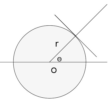
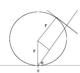
Figure 1: Simple examples for Cauchy formulae: circle centered on the origin, and circle ”resting” on the origin

In the elementary example of a circle centered on the origin with radius $r$ (Fig. 1), $M(\theta)$ is constant and equal to $r$ for all $\theta$. Its derivative is zero and Cauchy formulae give the standard results. The second example is slightly less trivial (Fig. 1) as $M(\theta)$ is not constant but equal to $r(1+\sin\theta)$. One of course recovers again the usual results:

$$L = \int_{0}^{2\pi}d\theta\ r(1+\sin\theta)=2\pi r$$

$$A = \frac{1}{2}\int_{0}^{2\pi}d\theta\ r^{2}[(1+\sin\theta)^{2}-\cos^{2}\theta]=\pi r^{2}.$$

It is interesting to note that Cauchy’s original motivations for deriving the formulae (40) and (41) actually came from a somewhat different context. He was interested in developing a method to compute the roots of certain algebraic equations as a convergent series and to compute an upper bound of the error made in stopping the series after a finite number of terms. It was in this connection that he proved a number of theorems concerning the length of the perimeter and the area enclosed by a closed convex curve in a plane. Anticipating the usefulness of his formulae in a variety of contexts and particularly in geometrical applications, he collected them in a self-contained ”Memoire” published by the ”Academie des Sciences” in 1850. It is worth pointing out that Cauchy’s formulae are of purely geometric origin without any probabilistic content. The idea of using these formulae in probabilistic context was first used by Crofton Cro whose work can be considered as one of the starting points of the subject of integral geometry, developed by Blaschke and his school during the years 1935-1939.

3.2 Support function of the convex hull of a discrete set of points in plane

Let $I=\{(x_{i},y_{i}),i=1,2,\ldots,N\}$ denote a set of $N$ points in a plane with coordinates $(x_{i},y_{i})$. Let $C$ denote the convex hull of $I$, i.e., the minimal convex polygon enclosing this set. This convex hull $C$ is a closed, smooth convex curve and hence we can apply Cauchy’s formulae in Eqs. (40) and (41) to compute its perimeter and area. However, to apply these formulae we first need to know the support function $M(\theta)$ associated with the convex hull $C$, as given by Eq. (39). This requires a knowledge of the coordinates $(X(s),Y(s))$ of a point, parametrized by $s$, on the convex polygon $C$. A crucial point is that one can compute this support function associated with the convex hull $C$ of $I$ just from the knowledge of the coordinates $(x_{k},y_{k})$ of the set $I$ itself and without requiring first to compute the coordinates $(X(s),Y(s))$ of the points on the convex hull $C$. Indeed the support function $M(\theta)$ associated with $C$ can be written as

$$M(\theta)=\max_{s\in C}\left\{X(s)\cos\theta+Y(s)\sin\theta\right\}=\max_{i\in I}\left\{x_{i}\cos\theta+y_{i}\sin\theta\right\}.$$ (42)

This simply follows from the fact that $M(\theta)$, the maximal extent of the convex polygon $C$ along $\theta$, is also the maximum of the projections of all points of the set $I$ along that direction $\theta$. Thus, the knowledge of the coordinates $(x_{k},y_{k})$ of any set $I$ is enough to determine the support function $M(\theta)$ of the convex hull $C$ associated with $I$ by Eq. (42).

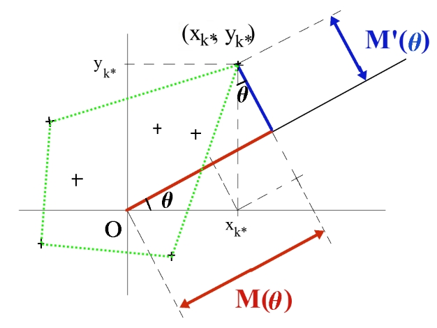
Figure 2: Support function $M(\theta)$ and its derivative $M^{\prime}(\theta)$ of the convex hull (dotted green lines) assocaited with a set of $7$ points.

We also note that, by definition of $M(\theta)$ in Eq. (42), for any fixed $\theta$ there will be a point $(x_{k^{*}},y_{k^{*}})$ in the set such that:

$$M(\theta)=x_{k^{*}}\cos\theta+y_{k^{*}}\sin\theta$$ (43)

Taking derivative of (43) with respect to $\theta$ gives

$$M^{\prime}(\theta)=-x_{k^{*}}\sin\theta+y_{k^{*}}\cos\theta$$ (44)

In other words, $M^{\prime}(\theta)$ is the distance between the point of the set giving the maximal projection $M(\theta)$ and the straight line with direction $\theta$, as illustrated in Figure 2.

3.3 A Simple illustration of the support function $M(\theta)$ of a triangle

To get familar with the support function $M(\theta)$ associated with a convex hull, let us consider a simple example of three points in a plane. The associated convex hull is evidently a triangle (Fig. 3) whose support function $M(\theta)$ and derivative $M^{\prime}(\theta)$ are drawn in Figures 4 and 4.

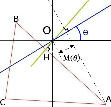
Figure 3: Triangle $ABC$ (in red), with the line of direction $\theta$ (in blue) and the line through $O$ perpendicular to $AB$

$M(\theta)$ is of course $2\pi$-periodic. A notable feature of its graph is the presence of angular points, corresponding to discontinuities of the derivative of $M(\theta)$. So, $M(\theta)$ appears piecewise smooth, with a derivative exhibiting a finite number of jump discontinuities. This finite number is, in the special case considered here, equal to three, the number of points in the set whose support function is $M(\theta)$. This is not by chance and the coincidence can be understood by returning to equations (43) and (44): within a given range of $\theta$, one of the vertices of the triangle $ABC$ will be giving the maximal projection on direction $\theta$ and will thus determine the value of $M(\theta)$, say:

$$M(\theta)=x_{A}\cos\theta+y_{A}\sin\theta,$$ (45)

Then, within the same range of $\theta$:

$$M^{\prime}(\theta)=-x_{A}\sin\theta+y_{A}\cos\theta.$$ (46)

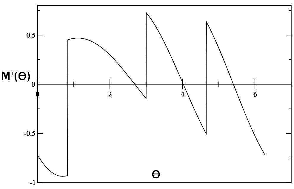
Figure 4: (a) Support function $M(\theta)$ of triangle $ABC$ and (b) its derivative $M^{\prime}(\theta)$

We can specify the range of angles $\theta$ on which equations (45 and 46) are valid. Let us indeed note that by the definition of $M(\theta)$, when $\theta$ corresponds to the perpendicular through the origin $O$ to the line segment $AB$, $A$ and $B$ have the same projection on direction $\theta$ (Fig. 3). In the $\theta^{-}$-limit, that is for angles approaching $\theta$ from below, the value of $M$ will be given by the projection of $A$, and the value of $|M^{\prime}(\theta)|$ by the length of the line segment $AH$ ($H$ being the foot of the perpendicular to $AB$ through $O$). In the $\theta^{+}$-limit, for angles slightly larger than $\theta$, the value of $M(\theta)$ will still be the common projection of $A$ and $B$ but $|M^{\prime}(\theta)|$ will be given by the length $BH$. Whence, as $\theta$ passes on the perpendicular to $AB$ through $O$, the support function $M$ will be continuous, while its derivative will have a jump discontinuity.

Indeed, looking at figure 3, and starting from $\theta=0$, we see that point $A$ gives the maximal projection on direction $\theta$, and the length of this projection decreases as $\theta$ increases, until the direction given by $\theta$ coincides with line $(OH)$, which is the perpendicular to $[AB]$ through the origin. At this point, as we have just noticed, $M(\theta)$ has an angular point: $B$ will then give the maximal projection, whose value will increase until $\theta$ corresponds to line $(OB)$ where $M(\theta)$ attains a local maximum before decreasing until $\theta$ coincides with the perpendicular to $[BC]$ through $O$, where $M(\theta)$ has a second angular point; and so on.

3.4 Cauchy formulae applied to a random sample

Let us now examine how the Cauchy formulae can be applied to determine the mean perimeter and the mean area of a convex hull associated with a set of $N$ points with coordinates $(x_{i},y_{i})$ in a plane chosen from some underlying probability distribution. The points may be independent or correlated.

For each $i$ and fixed $\theta$, let us define

$$z_{i}(\theta) = x_{i}\cos\theta+y_{i}\sin\theta$$ (47)

$$h_{i}(\theta) = -x_{i}\sin\theta+y_{i}\cos\theta.$$ (48)

$z_{i}$ is simply the projection of the $i$-th point in the sample on direction $\theta$ and $h_{i}$ its projection on the direction perpendicular to $\theta$. By definition (Eq. (42)):

$$M(\theta)=\mathop{\max}_{i}\{z_{i}(\theta)\}\equiv z_{k^{*}}(\theta)$$ (49)

for a certain index $k^{*}$.
One then has:

$$M^{\prime}(\theta)=h_{k^{*}}(\theta)$$ (50)

When the points $(x_{i},y_{i})$ are random variables, so is the index $k^{*}$ and subsequently both $M(\theta)$ and $M^{\prime}(\theta)$ are also random variables. Taking averages in Cauchy’s formulae ((40)) and ((41)) we get the mean perimeter and the mean area

$$\langle L\rangle = \int_{0}^{2\pi}d\theta\ \langle M(\theta)\rangle$$ (51)

$$\langle A\rangle = \frac{1}{2}\int_{0}^{2\pi}d\theta\ \left(\langle M^{2}(\theta)\rangle-\langle\left(M^{\prime}(\theta)\right)^{2}\rangle\right)$$ (52)

where $\langle\cdot\rangle$ indicates an average over all realisations of the points, and we assume that this operation commutes with the integration over $\theta$.

In the most general setting, let us also define

• $\mu_{\theta}$ be the probability density function of the maximum of the $z_{i}(\theta)$, i.e., of the random varibale $z_{k^{*}}(\theta)$

• $\rho_{\theta}$ be the probability density function of the index $k^{*}$ for which $z_{i}(\theta)$ becomes the maximum

• and $\sigma_{i,\theta}$ be the probability density function of the random variable $h_{i}(\theta)$ for a fixed $i$ and $\theta$,

then:

$$\langle M(\theta)\rangle = \int_{-\infty}^{\infty}\ z\ \mu_{\theta}(z)\ dz$$ (53)

$$\langle M^{2}(\theta)\rangle = \int_{-\infty}^{\infty}\ z^{2}\ \mu_{\theta}(z)\ dz$$ (54)

$$\langle\left(M^{\prime}(\theta)\right)^{2}\rangle = \int_{I}\int_{-\infty}^{\infty}\ h^{2}\ \rho_{\theta}(k)\ \sigma_{k,\theta}(h)\ dk\ dh$$ (55)

$$= \int_{I}\ \rho_{\theta}(k)\ \langle h_{k}^{2}(\theta)\rangle\ dk$$ (56)

With this formulation, it appears explicitly that random convex hulls are directly linked with extreme-value statistics, the study of extremes in samples of random variables. Indeed, when $I$ is finite and the $N$ points labelled by $i\in I$ are chosen independently and are identically distributed, for instance in $\mathbb{R}^{2}$, then $\mu_{\theta}$ is the distribution of the maximum of $N$ real-valued i.i.d random variables (namely the $z_{i}(\theta)$’s) — a classical example of EVS EVSG1 ; EVSG2 ; Gne ; EVSC . One can then use directly the results of the standard EVS of i.i.d random variables. On the other hand, when the points are correlated, we need to study the distribution of the maximum of a set of correlated random variables–a subject of much current interest as mentioned in the introduction. Here we need to go beyond i.i.d variables and take into acount the strong correlations between the random variables that changes the distribution of their maximum in a nontrivial way.

If the sample points are the vertices of an $N$-step 2-dimensional random walk, then the $z_{i}(\theta)$’s can be seen, for a fixed $\theta$ as the vertices of an $N$-step 1-dimensional random walk, and $\mu_{\theta}$ is the distribution of the maximum of such a walk. Note that in this case, $\rho_{\theta}$ is the distribution of the step at which the 1-dimensional random walk $z_{i}(\theta)$ attains its maximum DanSky ; Odly ; CMY ; Feller .

One can also consider cases when $I$ is not a discrete, finite set: e.g. the random set might be the trajectory $\mathcal{B}(\tau)=(x(\tau),y(\tau))$ of a planar Brownian motion at times $\tau\in I=[0,T]$. In such a case, both $z_{\tau}(\theta)$ and $h_{\tau}(\theta)$ are instances of 1-dimensional Brownian motion, and $\mu_{\theta}$ is the distribution of the maximum of 1-dimensional Brownian motion in $[0,T]$, $\rho_{\theta}$ is the distribution of the time at which 1-dimensional Brownian motion attains its maximum in $[0,T]$ (given by Lévy’s arcsine law Lev3 ), and $\sigma_{\tau,\theta}$ the propagator of 1-dimensional Brownian motion between $0$ and $\tau$ (i.e. the distribution of the position of a linear Brownian motion after a time $\tau$).

In the following section, we use this approach to compute the mean perimeter and the mean area of the convex hull of a set of $N$ indepedently chosen points in a plane. In Section 5, we will examine how the same approach can be adapted to compute the mean perimeter and the mean area of the convex hull of $n$ independent planar Brownian paths each of the same duration $T$.

4 Independent Points

4.1 General case

Let us consider here a sample of $N$ points drawn independently from a bivariate distribution:

$${\rm Prob}\left(x_{i}\in[x,x+dx],y_{i}\in[y,y+dy]\right)=p(x,y)\ dx\ dy,$$

Following the route explained in the previous section (Eqs. (47), (48)), we let:

$$z_{i}(\theta)=x_{i}\cos\theta+y_{i}\sin\theta,$$

and:

$$h_{i}(\theta)=-x_{i}\sin\theta+y_{i}\cos\theta$$

4.2 Isotropic cases

Let $(x_{1},y_{1}),(x_{2},y_{2}),\cdots,(x_{N},y_{N})$ be $N$ points in the plane, each drawn independently from a bivariate distribution $p(x,y)$ that is invariant under rotation, i.e., $p(x,y)=G(\sqrt{x^{2}+y^{2}})$. In such an isotropic case, the distribution of the support function $M(\theta)$ does not depend on $\theta$ and it is thus sufficient to set $\theta=0$ and hence $M_{N}\equiv M(0)$. The random variables $z_{i}(0)$ and $h_{i}(0)$ are just, respectively, the abscissa $x_{i}$ and ordinate $y_{i}$ of the points. Combining (51) and (53), we can then write the average perimeter of the convex hull

$$\langle L_{N}\rangle=2\pi\langle\mathop{\max}_{i}\{x_{i}\}\rangle\equiv 2\pi\langle M_{N}\rangle$$ (57)

It is useful to first define the cumulative distribution

$$F_{N}(M)=\text{Prob}[M_{N}\leq M].$$ (58)

For independent variables it follows that

$$F_{N}(M)=\left[\int_{-\infty}^{M}\ p_{X}(x)\ dx\right]^{N},$$ (59)

where $p_{X}(x)=\int_{-\infty}^{\infty}\ p(x,y)\ dy$ is the marginal of the first variable $X$. Thus, in a general isotropic case

$$\langle M_{N}\rangle = \int_{-\infty}^{\infty}\ M\ F_{N}^{\prime}(M)\ dM$$

$$\langle L_{N}\rangle = 2\pi\ N\int_{-\infty}^{\infty}\ M\ p_{X}(M)\left[\int_{-\infty}^{M}\ p_{X}(x)\ dx\right]^{N-1}\ dM$$ (60)

$$= 2\pi\ N\int_{-\infty}^{\infty}\ M\ p_{X}(M)\ F_{N-1}(M)\ dM$$

For the average area in the isotropic case, we can write it as (Eqs. (52), (54), (56)):

$$\langle A_{N}\rangle=\pi\langle M_{N}^{2}\rangle-\pi\langle y_{k^{*}}^{2}\rangle,$$ (61)

where $y_{k^{*}}$ is the ordinate of the point $(x_{k^{*}},y_{k^{*}})$ with the largest abscissa, i.e. satisfying:

$$x_{k^{*}}=\mathop{\max}_{i}\{x_{i}\}=M_{N}.$$

We can easily express the second moment of $M_{N}$ that appears in (61):

$$\langle M_{N}^{2}\rangle = \int_{-\infty}^{\infty}\ M^{2}F_{N}^{\prime}(M)\ dM$$ (62)

$$= N\int_{-\infty}^{\infty}\ M^{2}\ p_{X}(M)\ F_{N-1}(M)\ dM.$$ (63)

To compute the second term in (61), that is, the second moment of the ordinate of the point with largest abscissa, we first compute the probability density function $\hat{p}$ of this point, which is defined by:

$$\text{Prob}\ \left\{(x_{k^{*}},y_{k^{*}})\in\left[(x,y),(x+dx,y+dy)\right]\right\}=\hat{p}(x,y)\ dx\ dy$$ (64)

(Note that $F_{N}(M)=\int\ \hat{p}(M,y)\ dy$.)

It is not difficult to see that $\hat{p}(x_{k^{*}},y_{k^{*}})$ can be expressed as the probability density that one of the $N$ points has coordinates $(x_{k^{*}},y_{k^{*}})$ and the $N-1$ other points have abscissas less than $x^{*}$:

$$\hat{p}(x_{k^{*}},y_{k^{*}})=N\ p(x_{k^{*}},y_{k^{*}})\ \left[\int_{-\infty}^{x_{k^{*}}}\ p_{X}(x)\ dx\right]^{N-1}$$ (65)

Then:

$$\langle y_{k^{*}}^{2}\rangle=N\ \iint_{-\infty}^{\infty}\ y_{k^{*}}^{2}\ p(x_{k^{*}},y_{k^{*}})\ F_{N-1}(x_{k^{*}})\ dx_{k^{*}}\ dy_{k^{*}}$$ (66)

It now suffices to insert (63) and (66) in (61) to obtain a general expression for the average area of the convex hull of $N$ points drawn independently from an isotropic bivariate distribution $p$ with marginal $p_{X}$:

$$\langle A_{N}\rangle=N\ \pi\ \int_{-\infty}^{\infty}\ u^{2}\ p_{X}(u)\ F_{N-1}(u)\ du\\ -N\ \pi\ \iint_{-\infty}^{\infty}\ v^{2}\ p(u,v)\ F_{N-1}(u)\ du\ dv$$ (67)

The equations (60) and (67) are the main results of this subsection. They provide the exact mean perimeter and the mean area of the convex hull of $N$ independent points in a plane each drawn from an arbitrary isotropic distribution. As an example, let us consider the case of a Gaussian distribution where the general expressions can be further simplified. Let

$$p(x,y)=\frac{1}{2\pi}e^{-\frac{1}{2}(x^{2}+y^{2})}.$$ (68)

We then have:

$$p_{X}(x)=\frac{1}{\sqrt{2\pi}}\exp\left(-\frac{x^{2}}{2}\right)\equiv\phi(x)$$ (69)

and:

$$\int_{-\infty}^{x}\ p_{X}(x^{\prime})\ dx^{\prime}=\int_{-\infty}^{x}\ \phi(x^{\prime})\ dx^{\prime}\equiv\Phi(x)$$ (70)

Inserting these into equations (60) and (61), and performing suitable integrations by parts, we obtain:

$$\langle L_{N}\rangle = 4\ \pi\ \binom{N}{2}\ \int_{-\infty}^{\infty}\ \Phi^{N-2}(x)\ \phi^{2}(x)\ dx$$ (71)

$$\langle A_{N}\rangle = 3\ \pi\ \binom{N}{3}\ \int_{-\infty}^{\infty}\ \Phi^{N-3}(x)\ \phi^{3}(x)\ dx$$ (72)

which coincide with the expressions derived by Efron Ef using a rather different method.

4.3 Asymptotic behaviour of the average perimeter and area

To derive how the mean perimeter and the mean area behave for large $N$, we need to investigate the asymptotic large $N$ behavior of the two exact expressions in Eqs. (60) and (61). For the mean perimeter, since it is exactly identical to the maximum $M_{N}$ (upto a factor $2\pi$) of $N$ independent variables each distributed via the marginal $p_{X}(x)$, we can use the standard analysis used in EVS, which is summarized below. For the mean area, on the other hand, we need to go further. We will give a specific example of this asymptotic analysis of the mean area later.

Summary of standard extreme-value statistics

Let $z_{1},z_{2},\dots,z_{N}$ be independent, identically distributed random variables with probability density function $p(z)$, and let $M_{N}=\max_{\kappa=1..N}\left\{z_{\kappa}\right\}$ be their maximum. Then

$$F_{N}(M)=\text{Prob}\left(M_{N}\leq M\right)=\left[\int_{-\infty}^{M}\ p(z)\ dz\right]^{N}.$$

In the limit when $N$ becomes very large, the cumulative distribution function $F_{N}(M)$ exhibits one of the three following behaviours, according to the shape of the ”tails” of the parent distribution $p(z)$:

1. When the random variable $z$ has unbounded support and its distribution $p(z)$ has a faster than power law tail as $z\to\infty$. We will loosely refer to this as “Exponential tails”. Then, ”Exponential tails lead to a Gumbel-type law”

   $$p(z)\mathop{\sim}\limits_{z\rightarrow\infty}A\ e^{-z^{\alpha}}\ \rightarrow\quad F_{N}(M)\mathop{\sim}\limits_{N\rightarrow\infty}e^{-e^{-(M^{\alpha}-\log N)}}$$

2. ”Power-law tails lead to a Fréchet-type law”

   $$p(z)\mathop{\sim}\limits_{z\rightarrow\infty}A\ z^{-(\alpha+1)}\ \rightarrow\quad F_{N}(M)\mathop{\sim}\limits_{N\rightarrow\infty}e^{-\frac{A}{\alpha}\ N\ M^{-\alpha}}$$

3. ”Truncated tails (i.e. finite range $a$) lead to a Weibull-type law (with parameter $a$)”

   $$p(z)\mathop{\sim}\limits_{z\rightarrow a}A\ (a-z)^{\alpha-1}\ \rightarrow\quad F_{N}(M)\mathop{\sim}\limits_{N\rightarrow\infty}e^{-\frac{A}{\alpha}\ N\ (a-M)^{\alpha}}$$

In all three cases, the typical value of the maximum $M_{N}$ increases as $N$ increases: the larger the number of points, the further the maximum is pushed.

We will use these results for the general asymptotic behavior of the mean perimeter. However, before providing a summary of the asymptotic behavior for a general isotropic distribution, it is perhaps useful to consider two special cases in detail, one for the mean perimeter and one for the mean area, that will illustrate how one can carry out this asymptotic analysis. For the mean perimeter, we choose the parent distribution from the Weibull-type case and for the mean area we choose the Fréchet-type distribution. These choices are somewhat arbitrary, one could have equally chosen any other case for illustration.

Example 1: average perimeter in the ”Weibull-type” case

Let us consider $N$ points drawn independently inside a circle of radius $a$ from a distribution with Weibull-type tails:

$$p(x,y)\mathop{\sim}_{\sqrt{x^{2}+y^{2}}\rightarrow a}A\ (a-\sqrt{x^{2}+y^{2}})^{\gamma-1}.$$ (73)

Letting as before $F_{N}$ denote the cumulative distribution function of the maximum $M_{N}$ of the $x$-coordinates, an integration by parts yields:

$$\langle M_{N}\rangle = \int_{-a}^{a}\ x\ F_{N}^{\prime}(x)\ dx$$ (74)

$$= a-\int_{-a}^{a}\ F_{N}(x)\ dx$$

We focus on the second term of (74) and write:

$$I_{N}=\int_{-a}^{a}\ F_{N}(x)\ dx.$$

Then:

$$I_{N} = \int_{-a}^{a}\left[1-\int_{x}^{a}\ p_{X}(x^{\prime})\ dx^{\prime}\right]^{N}\ dx$$ (75)

$$= \int_{-a}^{a}\exp\left[N\ \log\left(1-\int_{x}^{a}\ p_{X}(x^{\prime})\ dx^{\prime}\right)\right]\ dx,$$ (76)

where as before we write $p_{X}(x)=\int\ p(x,y)\ dy$.

We now pick $0<\epsilon\ll 1$ such that

$$\text{for}\quad(a-\epsilon)<x<a,$$

$$p(x,y)\simeq A\ (a-\sqrt{x^{2}+y^{2}})^{\gamma-1}.$$

The idea being that when $N$ becomes large, some sample points will come closer and closer to the boundary (the circle of radius $a$) and consequently one can focus on the tails of the distribution. We therefore write:

$$I_{N}=I_{N}^{(1)}+I_{N}^{(2)}$$ (77)

with:

$$I_{N}^{(1)}=\int_{-a}^{a-\epsilon}\exp\left[N\ \log\left(1-\int_{x}^{a}\ p_{X}(x^{\prime})\ dx^{\prime}\right)\right]\ dx$$ (78)

and

$$I_{N}^{(2)}=\int_{a-\epsilon}^{a}\exp\left[N\ \log\left(1-\int_{x}^{a}\ p_{X}(x^{\prime})\ dx^{\prime}\right)\right]\ dx$$ (79)

It is possible to show that $I_{N}^{(1)}$ decreases exponentially with $N$ and is, as expected on heuristic grounds, subleading compared to $I_{N}^{(2)}$ which, as we are going to see, decreases as an inverse power in $N$.

The sample distribution $p(x,y)$ is rotationally invariant and bounded ($x^{2}+y^{2}\leq a^{2}$). Hence the marginal

$$p_{X}(x) = \int_{-\sqrt{a^{2}-x^{2}}}^{\sqrt{a^{2}-x^{2}}}\ p(x,y)\ dy$$ (80)

$$= 2\ \int_{0}^{\sqrt{a^{2}-x^{2}}}\ p(x,y)\ dy$$ (81)

Now for $x\lesssim a$, we have: $p(x,y)\sim A\ (a-\sqrt{x^{2}+y^{2}})^{\gamma-1}$. Consequently, setting $y=xu$ and considering that $(a-\epsilon)<x<a$:

$$p_{X}(x) \sim 2\ \int_{0}^{\sqrt{a^{2}-x^{2}}}\ A\ (a-\sqrt{x^{2}+y^{2}})^{\gamma-1}\ dy$$ (82)

$$\sim 2Ax\ \int_{0}^{\sqrt{\frac{a^{2}}{x^{2}}-1}}\ (a-x\ \sqrt{1+u^{2}})^{\gamma-1}\ du$$ (83)

$$\sim 2Aa\ \int_{0}^{\sqrt{\frac{2(a-x)}{a}}}\ (a-x)^{\gamma-1}\ du$$ (84)

$$\sim 2\ A\ \sqrt{2a}\ (a-x)^{\gamma-\frac{1}{2}}$$ (85)

We now proceed from equation (79):

$$I_{N}^{(2)} = \int_{a-\epsilon}^{a}\exp\left[N\ \log\left(1-\int_{x}^{a}\ p_{X}(x^{\prime})\ dx^{\prime}\right)\right]\ dx$$ (86)

$$\sim \int_{a-\epsilon}^{a}\exp\left[N\ \log\left(1-\int_{x}^{a}\ 2\ A\ \sqrt{2a}\ (a-x^{\prime})^{\gamma-\frac{1}{2}}\ dx^{\prime}\right)\right]\ dx$$

$$\sim \int_{a-\epsilon}^{a}\exp\left[N\ \log\left(1-\frac{4\ A\ \sqrt{2a}}{2\ \gamma+1}\ (a-x)^{\gamma+\frac{1}{2}}\right)\right]\ dx$$

$$\sim \int_{a-\epsilon}^{a}\exp-\left[\frac{4\ A\ N\ \sqrt{2a}}{2\ \gamma+1}\ (a-x)^{\gamma+\frac{1}{2}}\right]\ dx$$

To progress further, we perform the following change of variable:

$$u=\frac{4\ A\ N\ \sqrt{2a}}{2\ \gamma+1}\ (a-x)^{\gamma+\frac{1}{2}}$$ (87)

In the large $N$ limit in which we are working, this change of variable leads to:

$$I_{N}^{(2)} \sim \frac{2}{\left[4AN\sqrt{2a}\right]^{\frac{2}{1+2\gamma}}}\int_{0}^{\infty}\ e^{-u}\ \left[(2\gamma+1)\ u\right]^{\frac{1-2\gamma}{1+2\gamma}}\ du$$ (88)

$$\sim \frac{2\left(2\gamma+1\right)^{\frac{1-2\gamma}{1+2\gamma}}\ \Gamma\left(\frac{2}{2\gamma+1}\right)}{\left[4AN\sqrt{2a}\right]^{\frac{2}{1+2\gamma}}}$$

The combination of (88) with (74) and (57) yields the final result:

$$\langle L_{N}\rangle\mathop{\sim}_{n\rightarrow\infty}2\pi a-\frac{4\ \pi\left(2\gamma+1\right)^{\frac{1-2\gamma}{1+2\gamma}}\ \Gamma\left(\frac{2}{2\gamma+1}\right)}{\left[4AN\sqrt{2a}\right]^{\frac{2}{1+2\gamma}}}$$ (89)

To illustrate this asymptotic result for a concrete example, consider $N$ points drawn independently and uniformly from a unit disk

$$p(x,y)=\frac{1}{\pi}\ \Theta(1-x^{2}-y^{2}),$$ (90)

where $\Theta$ is the Heaviside step function.

In terms of our notations, this corresponds to:

$$a = 1,$$ (91)

$$A = \frac{1}{\pi},$$ (92)

$$\gamma = 1.$$ (93)

We find:

$$\langle L_{N}\rangle\mathop{\sim}_{N\rightarrow\infty}2\pi\ \left(1-\frac{\Gamma\left(\frac{2}{3}\right)\pi^{\frac{2}{3}}}{12^{\frac{1}{3}}\ N^{\frac{2}{3}}}\right),$$ (94)

in complete agreement with Rényi and Sulanke’s result Eq. (11)) RS2 . Note that for large $N$, the mean perimeter of the convex hull approaches $2\pi$, i.e., the convex hull approaches the bounding circle of radius unity of the disk. But it approaches very slowly, the correction term decreases for large $N$ only as a power law $\sim N^{-2/3}$. Actually, for this example of uniform distribution over a unit disk, one can also obtain simple and explicit expressions for the mean perimeter and the mean area starting from our general expressions in Eqs. (60) and (61). Skipping details, we get

Perimeter:

$$\langle L_{N}\rangle=2\pi\ \left[1-\int_{-1}^{1}\ F_{N}(M)\ dM\right]$$ (95)

Area:

$$\langle A_{N}\rangle=\pi\ \left[1-\frac{8}{3}\int_{-1}^{1}\ M\ F_{N}(M)\ dM\right]$$ (96)

where:

$$F_{N}(M)=\frac{1}{\pi}\ \left[\arcsin(M)+M\ \sqrt{1-M^{2}}\right]^{N}$$ (97)

One can also easily work out the asymptotic behavior of the mean area in this example using Eqs. (96) and (97) and we get

$$\langle A_{N}\rangle\mathop{\sim}_{N\rightarrow\infty}\pi\ \left(1-2\frac{\Gamma\left(\frac{2}{3}\right)2^{\frac{7}{3}}\pi^{\frac{2}{3}}}{3^{\frac{4}{3}}\ N^{\frac{2}{3}}}\right)$$ (98)

which, once again, agrees with Rényi and Sulanke’s result (Eq. (12)) RS2 . Note also that the mean area of the convex hull approaches, for large $N$, to the area of the unit disk. Notice also that the exponent of $N$, which governs the speed of convergence is the same for the area as for the perimeter — only the prefactor of the power of $N$ changes.

At this point it is also worth recalling the results of Hilhorst et al. Hilhorst regarding Sylvester’s problem . When $N$ becomes large, the convex hull of the $N$ points (conditioned to have all the $N$ points to be its vertices) lies in an annulus of width $\sim N^{-\frac{4}{5}}$ smaller than the $N^{-\frac{2}{3}}$ found in our case. This can be understood qualitatively by noticing that requiring the $N$ points to be on the convex hull will tend to increase the size of the hull and therefore push it closer to the boundary of the disk.

Example 2: average area in the ”Fréchet-type” case

Consider $N$ points drawn independently from an isotropic distribution with Fréchet-type tails:

$$p(x,y)\mathop{\sim}_{\sqrt{x^{2}+y^{2}}\rightarrow\infty}\frac{A}{(x^{2}+y^{2})^{\frac{\gamma+2}{2}}}.$$ (99)

Recalling equation (67), we start by its first term. Letting as before $F_{N}$ denote the cumulative distribution function of the maximum $M_{N}$ of the $x$-coordinates, we have:

$$\langle M_{N}^{2}\rangle=\int_{-\infty}^{\infty}\ x^{2}\ F_{N}^{\prime}(x)\ dx\equiv I_{N}.$$ (100)

With the same notation as previously:

$$F_{N}(x)=\left[1-\int_{x}^{\infty}\ p_{X}(x^{\prime})\ dx^{\prime}\right]^{N}$$ (101)

where as before we write $p_{X}(x)=\int\ p(x,y)\ dy$.

We pick $K\gg 1$ such that for

$$x\geq K,$$

$$p(x,y)\simeq\frac{A^{\prime}}{(x^{2}+y^{2})^{\frac{\gamma+2}{2}}}.$$

The idea being that when $N$ becomes large, sample points will disseminate further and further in the plane, and consequently one can focus on the tails of the distribution. We therefore write:

$$I_{N}=I_{N}^{(1)}+I_{N}^{(2)}$$ (102)

with:

$$I_{N}^{(1)}=\int_{-\infty}^{K}\ x^{2}\ F_{N}^{\prime}(x)\ dx$$ (103)

and

$$I_{N}^{(2)}=\int_{K}^{\infty}\ x^{2}\ F_{N}^{\prime}(x)\ dx$$ (104)

It is easy to show that $I_{N}^{(1)}$, as before, is subleading compared to $I_{N}^{(2)}$.

The sample distribution $p(x,y)$ is rotationally invariant and so:

$$p_{X}(x) = \int_{-\infty}^{\infty}\ p(x,y)\ dy$$ (105)

$$= 2\ \int_{0}^{\infty}\ p(x,y)\ dy$$ (106)

Now for $x\gg 1$, we have: $p(x,y)\sim\frac{A}{(x^{2}+y^{2})^{\frac{\gamma+2}{2}}}$. Consequently, setting $y=ux$ and considering cases when $x\gg 1$:

$$p_{X}(x) \sim 2\ \int_{0}^{\infty}\ \frac{A}{(x^{2}+y^{2})^{\frac{\gamma+2}{2}}}\ dy$$ (107)

$$\sim 2Ax\ \int_{0}^{\infty}\ \frac{1}{x^{\gamma+2}(1+u^{2})^{\frac{\gamma+2}{2}}}\ du$$ (108)

$$\sim \frac{A\sqrt{\pi}\Gamma\left(\frac{\gamma+1}{2}\right)}{x^{\gamma+1}\Gamma\left(\frac{\gamma}{2}+1\right)}$$ (109)

$$\sim \frac{C}{x^{\gamma+1}}$$ (110)

where we have set $C=A\sqrt{\pi}\frac{\Gamma\left(\frac{\gamma+1}{2}\right)}{\Gamma\left(\frac{\gamma}{2}+1\right)}$.

Now we can express $F_{N}(x)$ for large $x$ and large $n$:

$$F_{N}(x) \sim \left[1-\int_{x}^{\infty}\ \frac{C}{x^{\prime\gamma+1}}\ dx^{\prime}\right]^{N}$$ (111)

$$\sim \left[1-\frac{C}{\gamma\ x^{\gamma}}\right]^{N}$$

$$\sim e^{-\frac{NC}{\gamma\ x^{\gamma}}}$$

Whence, still for large $x$ and large $N$:

$$F_{N}^{\prime}(x)\sim\frac{NC}{x^{\gamma+1}}\ e^{-\frac{NC}{\gamma\ x^{\gamma}}}$$ (112)

We now insert (112) into (104), setting $u=\frac{NC}{\gamma\ x^{\gamma}}$:

$$I_{N}^{(2)} \sim \int_{0}^{\infty}\ \left(\frac{NC}{\gamma}\right)^{\frac{2}{\gamma}}\ u^{-\frac{2}{\gamma}}\ e^{-u}\,du$$ (113)

$$\sim \left(\frac{NC}{\gamma}\right)^{\frac{2}{\gamma}}\ \Gamma\left(1-\frac{2}{\gamma}\right)$$

Let us now examine the second term in equation (67). As before, we focus on the large-$x$ part of the integral, which will dominate. We rewrite it, so as to bring it down to the calculation that we have done in the previous paragraph:

$$N\int_{K}^{\infty}\int_{-\infty}^{\infty}\ y^{2}\ p(x,y)\ F_{N-1}(x)\ dx\ dy$$ (114)

$$= \int_{K}^{\infty}\ F_{N}^{\prime}(x)\ \frac{\int_{-\infty}^{\infty}\ y^{2}\ p(x,y)\ dy}{p_{X}(x)}\ dx$$

$$\sim \int_{K}^{\infty}\ F_{N}^{\prime}(x)\ x^{2}\ \frac{A}{C}\ \int_{-\infty}^{\infty}\ \frac{u^{2}}{(1+u^{2})^{\frac{\gamma+2}{2}}}\ du\ dx$$

$$\sim \frac{1}{\gamma-1}\ \int_{K}^{\infty}\ F_{N}^{\prime}(x)\ x^{2}\ dx$$

This last integral is, up to the factor $\frac{1}{\gamma-1}$, the same as (104); consequently, we obtain:

$$\langle A_{N}\rangle\mathop{\sim}_{N\rightarrow\infty}\left(1-\frac{1}{\gamma-1}\right)\ \int_{K}^{\infty}\ x^{2}\ F_{N}^{\prime}(x)\ dx,$$

which, combined to (113) and simplified, yields:

$$\langle A_{N}\rangle\mathop{\sim}_{N\rightarrow\infty}\frac{\gamma}{\gamma-1}\ \left(\frac{C}{\gamma}\right)^{\frac{2}{\gamma}}\Gamma\left(2\left(1-\frac{1}{\gamma}\right)\right)\ N^{\frac{2}{\gamma}}.$$ (115)

This coincides with the result of Carnal Ca .

Asymptotic results for general isotropic case:

The large $N$ asymptotic analysis for a general isotropic distribution, both for the mean perimeter and the mean area, can be done following the details presented in the above two examples. We just provide a summary here without repeating the details.

Average Perimeter:

• Exponential tails ($p(x,y)\sim Ae^{-(x^{2}+y^{2})^{\alpha/2}}$ when $(x^{2}+y^{2})\rightarrow\infty$)

  $$\langle L_{N}\rangle\sim 2\pi\log^{1/\alpha}N$$

• Power-law tails ($p(x,y)\sim\frac{A}{(x^{2}+y^{2})^{(\frac{\gamma+1}{2})}}$):

  $$\langle L_{N}\rangle\sim 2\pi\left(\dfrac{A\,B(\frac{1}{2},\frac{\gamma+1}{2})}{\gamma}\right)^{\frac{1}{\gamma}}\Gamma\left(1-\frac{1}{\gamma}\right)\,N^{\frac{1}{\gamma}},$$

  where $B(x,y)$ is the beta function.

• Truncated tails ($p(x,y)\sim A(a-\sqrt{x^{2}+y^{2}})^{\gamma-1}$):

  $$\langle L_{N}\rangle\sim 2\pi\left(a-\dfrac{f(a,\gamma)}{N^{\frac{2}{2\gamma+1}}}\right),$$

  with

  $$f(a,\gamma)=\dfrac{(\gamma+\frac{1}{2})^{\frac{1-2\gamma}{1+2\gamma}}\Gamma(\frac{2}{1+2\gamma})}{(2A\sqrt{2a})^{\frac{2}{1+2\gamma}}}$$

Therefore, we do find as expected the distinction between the three different universality classes of extreme-value statistics. The sets of independent points drawn from distributions with exponential tails have, on average when $N$ becomes large, a convex hull whose perimeter increases more slowly (in powers of $\log N$) than sets drawn from distribution with power-law tails (for which the growth of the perimeter is in powers of $N$), which reveals the lesser probability of having points very far from the origin in exponential-tailed distributions than in power-law tailed distributions.

Average area:

• Exponential tails:

  $$\langle A_{N}\rangle\sim\pi\log^{\frac{2}{\alpha}}N$$

• Power-law tails:

  $$\langle A_{N}\rangle\sim\pi(\frac{\gamma}{\gamma-1})\left(\dfrac{AB(\frac{1}{2},\frac{\gamma+1}{2})}{\gamma}\right)^{\frac{2}{\gamma}}\Gamma\left(2-\frac{2}{\gamma}\right)N^{\frac{2}{\gamma}}$$

• Truncated tails :

  $$\langle A_{N}\rangle\sim\pi a^{2}\left(1-\dfrac{8\ f(a,\gamma)}{3\ N^{\frac{2}{2\gamma+1}}}\right),$$

  with

  $$f(a,\gamma)=\dfrac{(\gamma+\frac{1}{2})^{\frac{1-2\gamma}{1+2\gamma}}\Gamma(\frac{2}{1+2\gamma})}{(2A\sqrt{2a})^{\frac{2}{1+2\gamma}}}$$

We find for the area the same characteristics as for the perimeter as far as the relative growths of convex hulls are concerned, depending on the shape of the initial distribution of the points. It is particularly worth noting that, in the case of exponential-tailed distributions, the asymptotic behaviour of the average perimeter and area of the convex hull correspond to the geometrical quantities of a circle centered on the origin and with radius $\log^{\frac{1}{\alpha}}N$ ($\alpha$ being the characteristic exponent of the initial distribution’s exponential tails).

4.4 A non-isotropic case: points distributed uniformly in a square

Let us now examine a non-isotropic case: computing the average perimeter of the convex hull of $N$ independent points distributed uniformly in a square of side $a$. The bivariate probability density of the sample can be written as:

$$p(x,y)=\frac{1}{a^{2}}\Theta(\frac{a^{2}}{4}-x^{2})\Theta(\frac{a^{2}}{4}-y^{2}),$$ (116)

where $\Theta$ is the Heaviside step function.

We will consider, as described in the introductory part of this section, the projection of the sample on the line through the origin making an angle $\theta$ with the $x$-axis. We write the random variable corresponding to the projection of a sample point $z\equiv x\cos\theta+y\sin\theta$. Its density will be given by :

$$q(z)=\frac{1}{a^{2}}\iint_{-\frac{a}{2}}^{\frac{a}{2}}\ \delta(z-x\cos\theta-y\sin\theta)\Theta(\frac{a^{2}}{4}-x^{2})\Theta(\frac{a^{2}}{4}-y^{2})\ dx\ dy,$$ (117)

where $\delta$ is the Dirac delta function.

Using the symmetry of the square, we can focus on $0\leq\theta\leq\frac{\pi}{4}$ and write

$$x=\frac{z-y\sin\theta}{\cos\theta}.$$

This enables us to simplify (117):

$$q(z)=\frac{1}{a^{2}\cos\theta}\int_{-\frac{a}{2}}^{\frac{a}{2}}\Theta(\frac{a^{2}}{4}-\left(\frac{z-y\sin\theta}{\cos\theta}\right)^{2})\Theta(\frac{a^{2}}{4}-y^{2})\ dy.$$ (118)

Enforcing the condition that any point of the sample lies inside the square and thus making the Heaviside functions non-zero, we have:

(i) $$-\frac{a}{2}\leq y\leq\frac{a}{2}$$ (119)

(ii) $$-\frac{a}{2}\leq\frac{z-y\sin\theta}{\cos\theta}\leq\frac{a}{2}$$ (120)

$$\therefore \max\left(-\frac{a}{2},\frac{z-\frac{a}{2}\cos\theta}{\sin\theta}\right)\leq y\leq\min\left(\frac{a}{2},\frac{z+\frac{a}{2}\cos\theta}{\sin\theta}\right)$$ (121)

and:

$$-\frac{a}{2}(\cos\theta+\sin\theta)\leq z\leq\frac{a}{2}(\cos\theta+\sin\theta)$$ (122)

There will be 3 cases:

1. For

   $$-\frac{a}{2}(\cos\theta+\sin\theta)\leq z\leq\frac{a}{2}(\sin\theta-\cos\theta),$$

   the $y$-coordinate will vary between $-\frac{a}{2}$ and $\frac{z+\frac{a}{2}\cos\theta}{\sin\theta}$ and therefore:

   $$q(z)=\frac{z+\frac{a}{2}(\cos\theta+\sin\theta)}{a^{2}\cos\theta\sin\theta}.$$ (123)

2. For

   $$\frac{a}{2}(\sin\theta-\cos\theta)\leq z\leq\frac{a}{2}(\cos\theta-\sin\theta),$$

   the $y$-coordinate will vary between $-\frac{a}{2}$ and $\frac{a}{2}$ and therefore:

   $$q(z)=\frac{1}{a\cos\theta}.$$ (124)

3. For

   $$\frac{a}{2}(\cos\theta-\sin\theta)\leq z\leq\frac{a}{2}(\cos\theta+\sin\theta)$$

   the $y$-coordinate will vary between $\frac{z-\frac{a}{2}\cos\theta}{\sin\theta}$ and $\frac{a}{2}$ and therefore:

   $$q(z)=\frac{\frac{a}{2}(\cos\theta+\sin\theta)-z}{a^{2}\cos\theta\sin\theta}.$$ (125)

To lighten the notation, let us write henceforth:

$$a_{\theta} = \frac{a}{2}(\cos\theta+\sin\theta)$$ (126)

$$b_{\theta} = a^{2}\cos\theta\sin\theta$$ (127)

Denoting as before by $M_{N}(\theta)$ the value of the support function of the sample at angle $\theta$, that is, the value of the maximal projection on direction $\theta$, we have:

$$\langle M_{N}(\theta)\rangle = \int_{-a_{\theta}}^{a_{\theta}}\ z\ F^{\prime}_{\theta,N}(z)\ dz$$ (128)

$$= \left[zF^{\prime}_{\theta,N}(z)\right]_{-a_{\theta}}^{a_{\theta}}-\int_{-a_{\theta}}^{a_{\theta}}\ F_{\theta,N}(z)\ dz$$ (129)

$$= a_{\theta}-I_{\theta},$$ (130)

where:

$$F_{\theta,N}(z) = \left[\int_{-a_{\theta}}^{z}\ q(z^{\prime})\ dz^{\prime}\right]^{N}$$ (131)

$$I_{\theta} = \int_{-a_{\theta}}^{a_{\theta}}\ F_{\theta,N}(z)\ dz$$ (132)

To compute $I_{\theta}$ we make use of our knowledge of $q(z)$ (Eqs. (123), (124), (125)) and we obtain:

$$\langle M_{N}(\theta)\rangle=a_{\theta}-\frac{\sin\theta\tan^{N}\theta}{2^{N-1}(2N+1)}-\frac{\cos\theta}{2^{N}(N+1)}\left[(2-\tan\theta)^{N+1}-\tan^{N+1}\theta\right]\\ -\sqrt{b_{\theta}\tan\theta}\ {}_{2}F_{1}\left(\frac{1}{2},-N;\frac{3}{2};\frac{\tan\theta}{2}\right),$$ (133)

${}_{2}F_{1}$ being a hypergeometric function.

Using known facts about the asymptotic behaviour of hypergeometric series AbSteg , $\langle M_{N}(\theta)\rangle$ can be seen to behave in the following way for large $N$:

$$\langle M_{N}(\theta)\rangle\sim a_{\theta}-\sqrt{\frac{\pi b_{\theta}}{2N}}+o\left(\frac{1}{\sqrt{N}}\right)$$ (134)

This then yields the desired result:

$$\langle L_{N}\rangle = 8\int_{0}^{\frac{\pi}{4}}\ \langle M_{N}(\theta)\rangle$$ (135)

$$\sim 4\ a\left(1-\pi\frac{\Gamma\left(\frac{3}{4}\right)}{\Gamma\left(\frac{1}{4}\right)\ \sqrt{N}}\right).$$ (136)

This is the same as Rényi and Sulanke’s RS2 , which they obtained from a different approach. Note that, as in the case of points distributed uniformly inside a disk, the average perimeter of the convex hull tends to that of the boundary of the support — here $4a$, the perimeter of the square — when the number $N$ of points becomes large. However, the convergence here is slower than for a support with a smooth boundary like the disk: $N^{-\frac{1}{2}}$ versus $N^{-\frac{2}{3}}$. One can think that, physically and statistically, it is somehow ”more difficult” for the points of the sample to reach inside the corners of the square, making the convergence of the convex hull towards the square all the more slower.

5 Correlated Points: One or more Brownian Motions

As mentioned before, one of the advantages of the support function approach that we use in this paper is its generality: it can be applied to samples with correlations as well as to samples of independent points. In this Section, we study, using this method, the convex hull of $n$ planar Brownian paths, a topic that has so far been considered only in the $n=1$ case Lev ; El ; Ta ; Go ; Go2 .

Beyond its interest from a theoretical point of view, the study of the convex hull of $n$ planar Brownian paths can be motivated by a question of particular relevance to the conservation of animal species in their habitat, as we shall see before giving the details of results.

5.1 Planar Brownian paths and home-range

A question that ecologists often face, in particular in designing a conservation area to preserve a given animal population ConsPlan , is how to estimate the home-range of this animal population. Roughly speaking this means the following. In order to survive over a certain length of time, the animals need to search for food and hence explore a certain region of space. How much space one needs to assign for a group of say $n$ animals? For instance, in the case of species having a nest to which they return, say, every night, the ”length of time” is just the duration of a day. In ecology, the home range is simply defined as the territory explored by the herd during its daily search for food over a fixed length of time. Different methods are used to estimate this territory, based on the monitoring of the animals’ positions Worton ; Luca . One of these consists in simply the minimum convex polygon enclosing all monitored positions, called the convex hull. While this may seem simple minded, it remains, under certain circumstances, the best way to proceed Folia .

The monitored positions, for one animal, will appear as the vertices of a path whose statistical properties will depend on the type of motion the animal is performing. In particular, during phases of food searching known as foraging, the monitored positions can be described as the vertices of a random walk in the plane ERW ; BRW ; EKRW . For animals whose daily motion consists mainly in foraging, quantities of interest about their home range, such as its perimeter and area, can be estimated through the average perimeter and area of the convex hull of the corresponding random walk (Fig. 5).

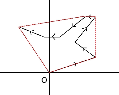
Figure 5: Convex hull of a 7-step random walk

If the recorded positions are numerous (which might result from a very fine and/or long monitoring), the number of steps of the random walker becomes large and to a good approximation the trajectory of a discrete-time planar random walk (with finite variance of the step sizes) can be replaced by a continuous-time planar Brownian motion of a certain duration $T$. (fig. 6).

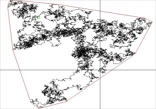
Figure 6: Convex hull of planar Brownian motion

The home range of a single animal can thus be characterized by the mean perimeter and area of the convex hull of a planar Brownian motion of duration $T$ starting at origin $O$. Both ‘open’ (where the endpoint of the path is free) and ‘closed’ paths (that are constrained to return to the origin in time $T$) are of interest. The latter corresponds, for instance, to an animal returning every night to its nest after spending the day foraging in the surroundings. As we have seen in our review of existing results, the average perimeter and area of the convex hull of an open Brownian path are known Ta ; El , as is the average perimeter for a closed path Go . It seems natural and logical to seek an extension of these results to an arbitrary number of paths (fig. 7), both from a theoretical point of view and from an ecological one, since many animals live in herds. We show first how to use the support-function method for $n=1$ planar Brownian paths and then for $n>1$.

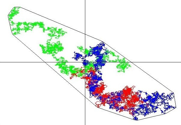
Figure 7: Convex hull of 3 independent, closed Brownian paths, starting at the origin $O$.

5.2 Convex hull of a planar Brownian path

We consider here a planar Brownian path of duration $T$, starting from the origin $O$:

$$\mathcal{B}(\tau)=(x(\tau),y(\tau))$$

with

$$0\leq\tau\leq T,$$

$x(\tau)$ and $y(\tau)$ being standard 1-dimensional Brownian motions of duration $T$ obeying the following Langevin equations:

$${\dot{x}}(\tau)=\eta_{x}(\tau)$$

and

$${\dot{y}}(\tau)=\eta_{y}(\tau)$$

where $\eta_{x}(\tau)$ and $\eta_{y}(\tau)$ are independent Gaussian white noises, with zero mean and delta-correlation:

$$\langle\eta_{.}(\tau)\eta_{.}(\tau^{\prime})\rangle=\delta(\tau-\tau^{\prime}).$$

Let us note incidentally that this implies:

$$\langle x^{2}(\tau)\rangle=\tau$$

and

$$\langle y^{2}(\tau)\rangle=\tau$$ (137)

.

Fix a direction $\theta$. We use as before (Eqs. (47) and (48)) the projection on direction $\theta$:

$$z_{\theta}(\tau)=x(\tau)\cos\theta+y(\tau)\sin\theta$$

and

$$h_{\theta}(\tau)=-x(\tau)\sin\theta+y(\tau)\cos\theta.$$

Now, $z_{\theta}$ and $h_{\theta}$ are two independent 1-dimensional Brownian motion (each of duration $T$), parametrized by $\theta$. It thus appears that $M(\theta)$ is simply the maximum of the 1-dimensional Brownian motion $z_{\theta}(\tau)$ on the interval $\tau\in[0,T]$, i.e.,

$$M(\theta)=\mathop{\max}_{\tau\in[0,T]}[z_{\theta}(\tau)].$$

Furthermore, if we write $\tau^{*}$ the time at which this maximum is attained, then:

$$M(\theta)=z_{\theta}(\tau^{*})=x(\tau^{*})\cos\theta+y(\tau^{*})\sin\theta.$$

Deriving with respect to $\theta$ gives:

$$M^{\prime}(\theta)=-x(\tau^{*})\sin\theta+y(\tau^{*})\cos\theta=h_{\theta}(\tau^{*}).$$

In words, if $M(\theta)$ is the maximum of the first Brownian motion $z_{\theta}(\tau)$, $M^{\prime}(\theta)$ corresponds to the value of the second, independent motion $h_{\theta}(\tau)$ at the time $\tau=\tau^{*}$ when the first one attains its maximum. (cf. Fig. 8 and 8).

In particular, when $\theta=0$, $z_{0}(\tau)=x(\tau)$ and $h_{0}(\tau)=y(\tau)$, and $M(0)$ is then the maximum of $x(\tau)$ on the interval $\tau\in[0,T]$ while $M^{\prime}(0)=y(\tau^{*})$ is the value of $y$ at the time $\tau^{*}$ when $x$ attains its maximum.

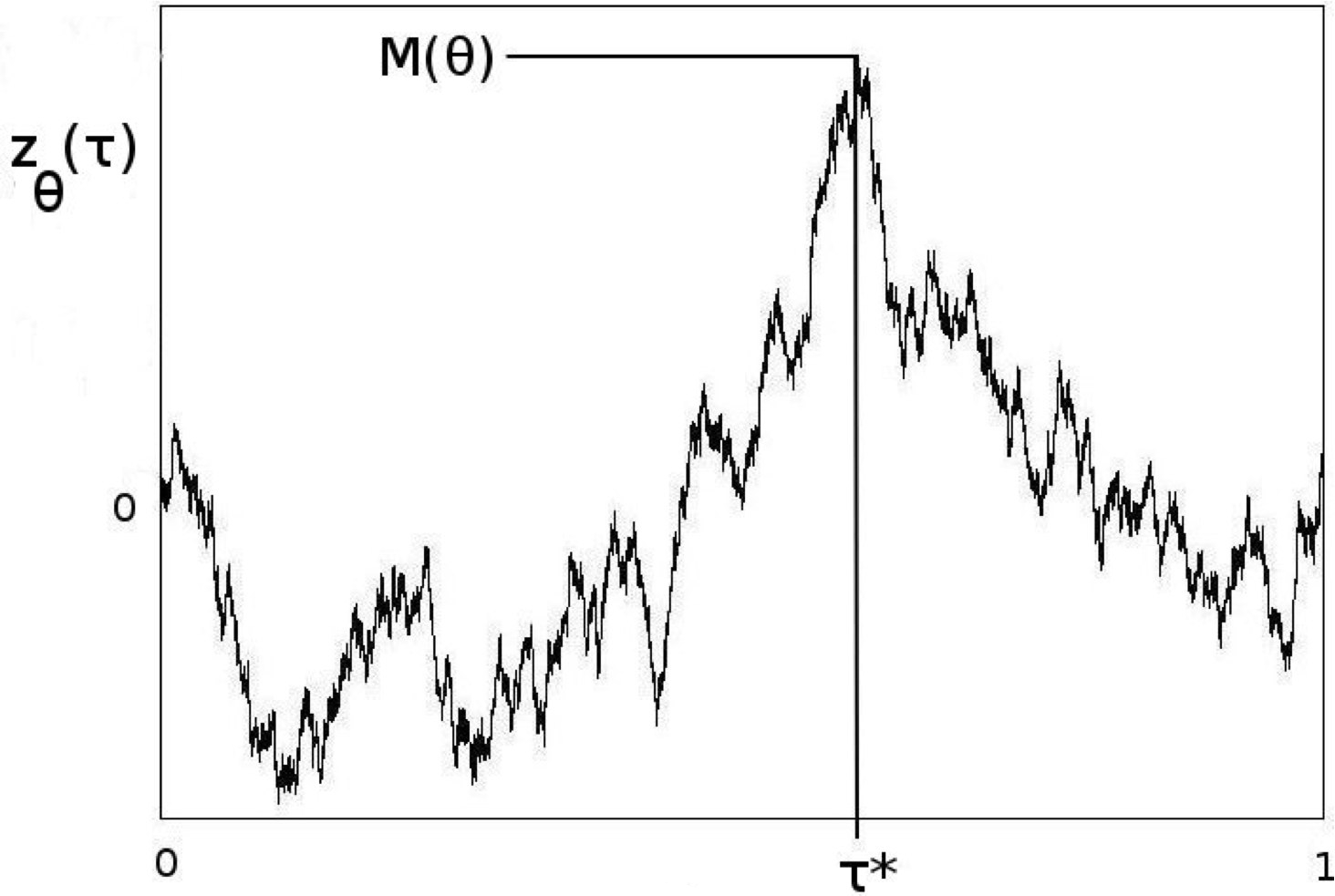
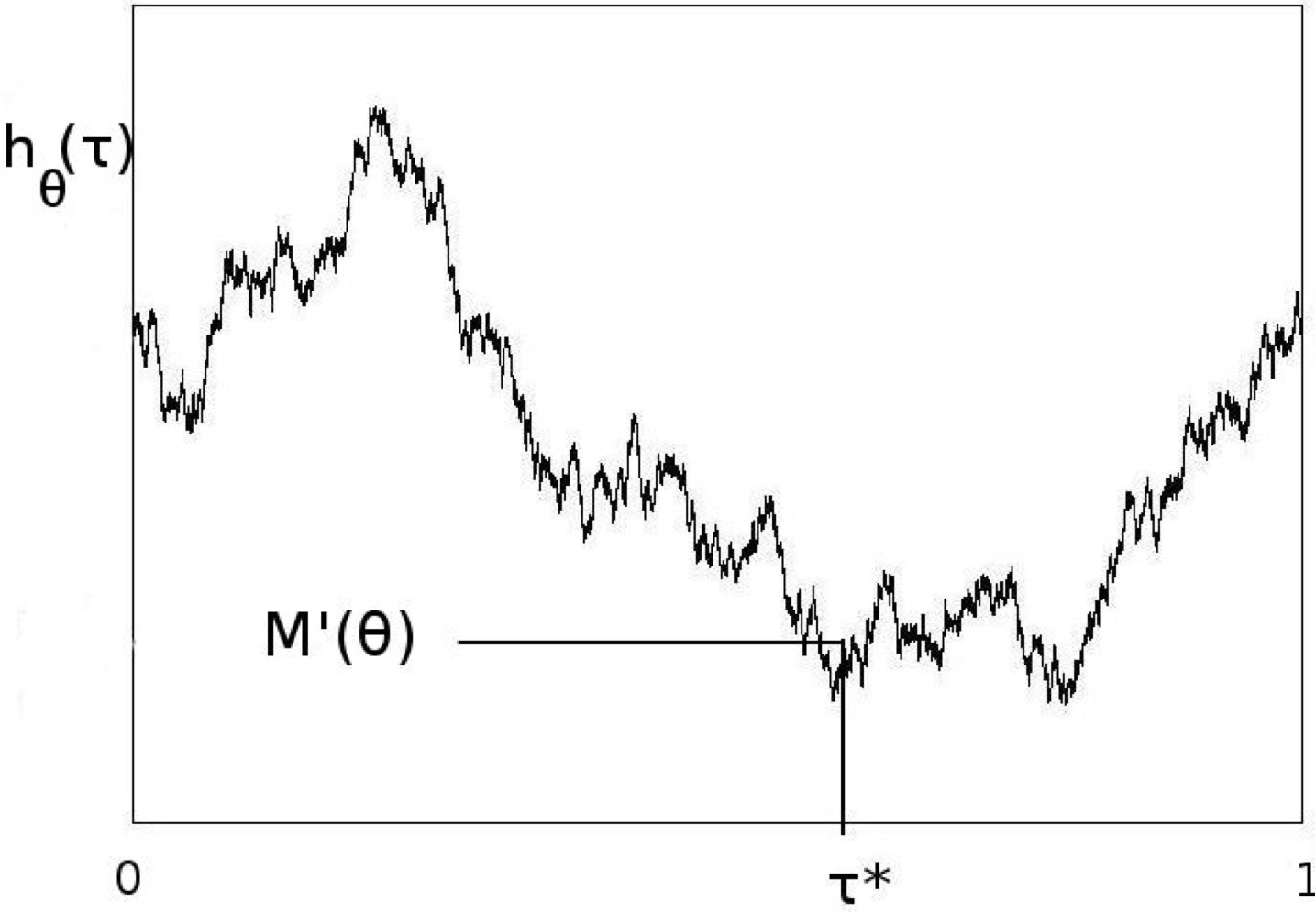
Figure 8: (a) Time $\tau^{*}$ when the maximum $M(\theta)$ of $z_{\theta}(\tau)$ is attained and (b) corresponding value $M^{\prime}(\theta)=h_{\theta}(\tau^{*})$

Recall that in isotropic cases, Cauchy’s formulae (Eqs. (51) and (52)) simplify to:

$$\langle L\rangle = 2\pi\ \langle M(0)\rangle$$ (138)

$$\langle A\rangle = \pi\left(\langle[M(0)]^{2}\rangle-\langle[M^{\prime}(0)]^{2}\rangle\right).$$ (139)

The planar motion that we are considering here is assumed to be isotropic and we will thus use this version of the formulae.

The distribution of the maximum of a 1-dimensional Brownian motion $x(\tau)$ on $[0,T]$ is known, and given by the cumulative distribution function:

$$F(M)={\rm Prob}[M(0)\leq M]=\ \text{erf}\left(\frac{M}{\sqrt{2T}}\right),$$ (140)

with

$${\rm erf}(z)=\frac{2}{\sqrt{\pi}}\,\int_{0}^{z}e^{-u^{2}}\,du.$$

The first two moments of this distribution are readily computed:

$$\langle M(0)\rangle=\sqrt{\frac{2T}{\pi}}$$

and

$$\langle[M(0)]^{2}\rangle=T.$$

Equation (138) then yields the average perimeter of the convex hull of a planar Brownian path,

$$\langle L\rangle=\sqrt{8\pi T}.$$ (141)

It is slightly more complex to compute the average area enclosed by the convex hull as one then needs to compute $\langle[M^{\prime}(0)]^{2}\rangle$. Let us first recall (Eq. (137)) that for a given $\tau^{*}$,

$$E[y^{2}(\tau^{*})]=\tau^{*}$$

(since $y$ is a standard Brownian motion), the expectation being taken over all possible realisations of $y$ at fixed $\tau^{*}$. But $\tau^{*}$ is itself a random variable, since it is the time at which the first process, $x$, attains its maximum. One therefore also has to average over the probabability density of $\tau^{*}$ (which is given by Lévy’s celebrated arcsine law: $\rho_{1}(\tau^{*})=[\tau^{*}(T-\tau^{*})]^{-1/2}/\pi$); this leads to:

$$\langle[M^{\prime}(0)]^{2}\rangle=\langle\tau^{*}\rangle=T/2;$$

whence one obtains, via equation (139), the exact expression for the average area enclosed by the convex hull of the motion:

$$\langle A\rangle=\frac{\pi T}{2}.$$ (142)

If we now consider a closed Brownian path in the plane, that is, one constrained to return to the origin after time $T$, the reasoning is completely similar, but for $x(\tau)$ and $y(\tau)$ which are now Brownian bridges of duration $T$: both start from the origin and are constrained to return to it at time $T$:

$$x(0)=x(T)=0$$

$$y(0)=y(T)=0.$$

The distribution of the maximum of a Brownian bridge is also known, and its first two moments are given by:

$$\langle M(0)\rangle=\sqrt{\frac{\pi T}{8}}$$

and

$$\langle[M(0)]^{2}\rangle=\frac{T}{2}.$$

Equation (138) gives us as before the average perimeter of the convex hull:

$$\langle L\rangle=\sqrt{\frac{\pi^{3}T}{2}}.$$ (143)

To compute the average area enclosed by the convex hull $y(\tau)$, let us first note that for a Brownian bridge, at a fixed time $\tau^{*}$:

$$E[y^{2}(\tau^{*})]=\frac{\tau^{*}(T-\tau^{*})}{T}.$$

Let us then recall another well-known result: the probability density of $\tau^{*}$ is uniform. Thus, averaging on $\tau^{*}$, with uniform distribution $\rho_{1}(\tau^{*})=1/T$, we obtain:

$$\langle M^{\prime}(0)^{2}\rangle=\langle y^{2}(\tau^{*})\rangle=\frac{T}{6}.$$

Finally, as before, equation (139) leads us to an exact expession for the average area enclosed by the convex hull of a 2d Brownian bridge:

$$\langle A\rangle=\frac{\pi T}{3}.$$ (144)

Results (141) and (142) had been computed by M. El Bachir El , using the same approach as here, hinted at by L. Takács Ta . Equation (143) is given by A. Goldman. The last result, (144), is, to the best of our knowledge, new, as are those in the next paragraph, regarding the convex hull of several planar Brownian motions.

5.3 Convex hull of $n$ planar Brownian paths

As mentioned earlier, the method can then be generalized to $n$ independent planar Brownian paths, open or closed. We now have two sets of $n$ Brownian paths: $x_{j}(\tau)$ and $y_{j}(\tau)$ ($j=1,2,\ldots,n$). All paths are independent of each other. Since isotropy holds, we can still use Eqs. (138) and (139), except that $M(0)$ now denotes the global maximum of a set of $n$ independent one dimensional Brownian paths (or bridges for closed paths) $x_{j}(\tau)$ ($j=1,2,\ldots,n$), each of duration $T$,

$$M(0)=\max_{1\leq j\leq n}\,\max_{0\leq\tau\leq T}\left[x_{1}(\tau),x_{2}(\tau),\ldots,x_{n}(\tau)\right].$$ (145)

Let $j_{*}$ and $\tau^{*}$ denote the label of the path and the time at which this global maximum is achieved. Then, using argument similar to the $n=1$ case, it is easy to see that $M^{\prime}(0)=y_{j_{*}}(\tau^{*})$, i.e., the position of the $j_{*}$-th $y$ path at the time when the $x$ paths achieve their global maximum.

To compute the first two moments of $M(0)$, we first compute the distribution $P_{n}[M(0),T]$ of the global maximum of $n$ independent Brownian paths (or bridges) $x_{j}(\tau)$. This is a standard extreme value calculation.

5.4 Open paths

Consider first $n$ open Brownian paths. It is easier to compute the cumulative probability,

$$F_{n}(M)={\rm Prob}[M(0)\leq M].$$

Since the Brownian paths are independent, it follows that

$$F_{n}(M)=[F(M)]^{n},$$

where

$$F(M)={\rm erf}\left(\frac{M}{\sqrt{2T}}\right)$$

for a single path mentioned before.

Knowing this cumulative distribution $F_{n}(M(0))$, the first two moments $\langle M(0)\rangle$ and $\langle[M(0)]^{2}\rangle$ can be computed for all $n$. Using the result for $\langle M(0)\rangle$ in Eq. (138) gives us the mean perimeter, $\langle L_{N}\rangle=\alpha_{n}\sqrt{T}$ with

$$\alpha_{N}=4n\sqrt{2\pi}\int_{0}^{\infty}du\ u\ e^{-u^{2}}\left[\text{erf}\left(u\right)\right]^{n-1}.$$ (146)

The first few values are:

$$\alpha_{1} = \sqrt{8\pi}=5.013..,$$

$$\alpha_{2} = 4\sqrt{\pi}=7.089..$$

$$\alpha_{3} = 24\,\frac{{\rm tan}^{-1}\left(1/\sqrt{2}\right)}{\sqrt{\pi}}=8.333..$$

(see Fig. 11 for a plot of $\alpha_{n}$ vs. $n$).
For large $n$, one can analyse the integral in Eq. (146) by the saddle point method giving:

$$\alpha_{n}\sim 2\pi\sqrt{2\log n}.$$ (147)

(Details of the analysis are given in appendix C)
This logarithmic dependence on $n$ is thus a direct consequence of extreme value statistics EVSG2 and the calculation of the mean perimeter of the convex hull of $n$ paths is a nice application of the extreme value statistics.

To compute the mean area, we need to calculate $\langle[M^{\prime}(0)]^{2}\rangle$ in Eq. (139). We proceed as in the $n=1$ case. For a fixed label $j$ and fixed time $\tau$:

$$E[y_{j}^{2}(\tau)]=\tau,$$

which follows from the fact that $y_{j}(\tau)$ is simply a Brownian motion. Thus:

$$E[y_{j_{*}}^{2}(\tau^{*})]=\tau^{*}.$$

Next, we need to average over $\tau^{*}$ which is the time at which the global maximum in Eq. (145) happens. The probability density ${\rho}_{n}(\tau^{*})$ of the time $\tau^{*}$ of the global maximum of $n$ independent Brownian motions (each of duration $T$), to our knowledge, is not known in the probability literature. We were able to compute this exactly for all $n$ (details are given in appendix B). We find that

$$\rho_{n}(\tau^{*})=\frac{1}{T}\,f_{n}(\tau^{*}/T)$$

where the scaling function $f_{n}(z)$ is given by

$$f_{n}(z)=\frac{2n}{\pi\sqrt{z(1-z)}}\,\int_{0}^{\infty}dx\,x\,e^{-x^{2}}\,\left[{\rm erf}\left(x\sqrt{z}\right)\right]^{n-1}.$$ (148)

A plot of $f_{n}(z)$ for various values of $n$ is given in Fig. (9).

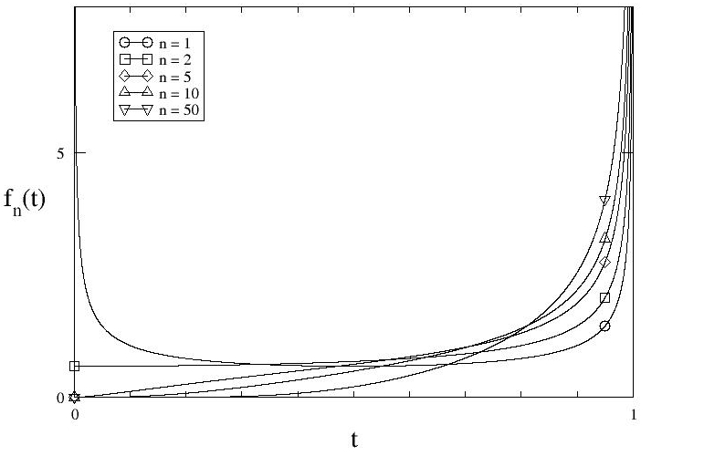
Figure 9: Probability density $f_{n}(t)$ of the time $t$ at which the global maximum of $n$ Brownian motions, each of unit duration, is attained, as given by the formula in Eq. (148).

It is easy to check that for $n=1$, it reproduces the arcsine law mentioned before.
Averaging over $\tau^{*}$ drawn from this distribution, we can then compute

$$\langle[M^{\prime}(0)]^{2}\rangle=\int_{0}^{T}\tau^{*}\rho_{n}(\tau^{*})\,d\tau^{*}.$$

Substituting this in Eq. (139) gives the exact mean area for all $n$, $\langle A_{n}\rangle=\beta_{n}T$ with

$$\beta_{n}={4n}\,{\sqrt{\pi}}\,\int_{0}^{\infty}du\ u\ \left[\text{erf}(u)\right]^{n-1}\left(ue^{-u^{2}}-g(u)\right)$$ (149)

where

$$g(u)=\frac{1}{2\sqrt{\pi}}\int_{0}^{1}\frac{e^{-{u^{2}}/{t}}\ dt}{\sqrt{t(1-t)}}.$$

For example, the first few values are given by:

$$\beta_{1} = \pi/2=1.570..$$ (150)

$$\beta_{2} = \pi=3.141..$$ (151)

$$\beta_{3} = \pi+3-\sqrt{3}=4.409..$$ (152)

(Fig. 11 shows a plot of $\beta_{n}$ vs $n$).
The large-$n$ analysis (details in appendix C) gives:

$$\boxed{\beta_{n}\sim 2\pi\ln n.}$$ (153)

5.5 Closed paths

For $n$ closed Brownian planar paths one proceeds in a similar way. The differences are:

• the cumulative distribution function of the maximum of a single 1-dimensional motion is not given by equation 140 but by:

  $$F(M)=1-e^{-\frac{2M^{2}}{T}}$$

• the propagator of the 1-dimensional motion obtained by projection on the $x$-axis is that of a Brownian bridge and so:

  $$E[y_{j_{*}}^{2}(\tau^{*})]=\frac{\tau^{*}(T-\tau^{*})}{T}$$

• the probabilty density of the time $\tau^{*}$ at which the maximum of $n$ 1-dimensional Brownian bridges occurs is given by (see details in appendix B):

  $$\rho_{n}(\tau^{*})=\frac{1}{T}g_{n}\left(\frac{\tau^{*}}{T}\right)$$

  where the scaling function $g_{n}(z)$ is given by

  $$g_{n}(z)=\frac{4n}{\sqrt{\pi}}\int_{0}^{\infty}\ u^{2}\ e^{-u^{2}}\ \left[1-e^{-4u^{2}\,z(1-z)}\right]^{n-1}\ du.$$ (154)

A plot of $g_{n}(z)$ for different $n$ is given in Fig. (10).

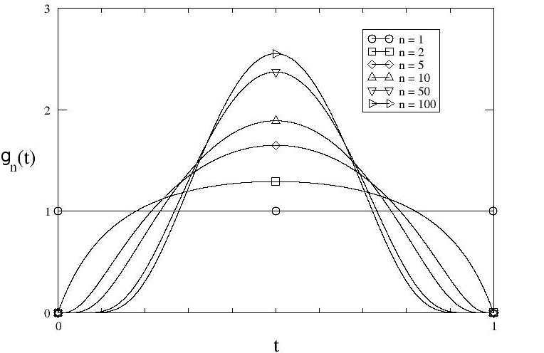
Figure 10: Probability density $g_{n}(t)$ of the time $t$ at which the global maximum of $n$ Brownian bridges, each of unit duration, is attained, as given by the formula in Eq. (154).

Following then the same route as for open paths, we find that the mean perimeter and area are given by:

$$\langle L_{n}\rangle=\alpha_{n}(c)\sqrt{T}$$

and

$$\langle A_{n}\rangle=\beta_{n}(c)T$$

where, for all $n$,

$$\alpha_{n}(c) = \frac{\pi^{3/2}}{\sqrt{2}}\sum_{k=1}^{n}\binom{n}{k}\frac{(-1)^{k+1}}{\sqrt{k}}$$ (155)

$$\beta_{n}(c) = \frac{\pi}{2}\left[\sum_{k=1}^{n}\frac{1}{k}-\frac{n}{3}+\frac{1}{2}\sum_{k=2}^{n}(-1)^{k}\,f(k)\right]$$ (156)

and

$$f(k)=\binom{n}{k}\,(k-1)^{-3/2}\left(k\tan^{-1}(\sqrt{k-1})-\sqrt{k-1}\right).$$

The first few values are:

$$\alpha_{1}(c) = \sqrt{\pi^{3}/2}=3.937.$$

$$\alpha_{2}(c) = \sqrt{\pi^{3}}(\sqrt{2}-1/2)=5.090..$$

$$\alpha_{3}(c) = \sqrt{\pi^{3}}(3/\sqrt{2}-3/2+1/\sqrt{6})=5.732..$$

and

$$\beta_{1}(c) = \pi/3=1.047..$$ (157)

$$\beta_{2}(c) = \pi(4+3\pi)/24=1.757..$$ (158)

$$\beta_{3}(c) = 2.250..$$ (159)

(see Fig. 11 for a plot of $\alpha_{n}(c)$ and $\beta_{n}(c)$ vs. $n$).
Large $n$ analysis (details in section C) shows that:

$$\boxed{\alpha_{n}(c)\sim\pi\sqrt{2\ln n}}$$ (160)

and

$$\boxed{\beta_{n}(c)\sim\frac{\pi}{2}\ln n,}$$ (161)

smaller respectively by a factor $1/2$ and $1/4$ than the corresponding results for open paths — as one’s intuition might suggest, given that a closed path is enforced to return to the origin.

5.6 Numerical simulations and discussion

We illustrate our analytical results on the convex hull of planar Brownian motion with some elementary numerical simulations. These require first to generate Brownian paths, and then to compute numerically the convex hull of the paths. Here we have used a simple algorithm known as Graham scan Grah .

Figure 11: Setting $T=1$, the analytical results for average perimeter $\alpha_{n}$ [Eq. (146), in red] and area $\beta_{n}$ [Eq. (149), in green] of $n$ open Brownian paths, and similarly the average perimeter $\alpha_{n}(c)$ [Eq. (155), in brown] and area $\beta_{n}(c)$ [Eq. (156), in purple] of $n$ closed Brownian paths, plotted against $n$. The symbols denote results from numerical simulations (up to $n=10$, with $10^{3}$ realisations for each point).

Let us recall the asymptotic behaviours of the exact formulae plotted in figure 11, which are given by equations (147), (153), (160) et (161).
For $n$ open Brownian paths:

$$\langle L_{n}\rangle \sim 2\pi\sqrt{2T\ln n}$$ (162)

$$\langle A_{n}\rangle \sim 2\pi T\ln n;$$ (163)

and for $n$ closed Brownian paths:

$$\langle L_{n}^{(c)}\rangle \sim\pi\sqrt{2T\ln n}$$ (164)

$$\langle A_{n}^{(c)}\rangle \sim\frac{\pi}{2}T\ln n.$$ (165)

In both cases, the ratio between the average value of the area of the convex hull and the square of the average value of the perimeter takes, asymptotically, the same value as in the case of a circle:

$$\frac{\langle A_{n}\rangle}{\langle L_{n}\rangle^{2}}\ \mathop{\simeq}_{n\rightarrow\infty}\ \frac{1}{4\pi}.$$ (166)

Thus, heuristically speaking, for large $n$, the convex hull of $n$ planar Brownian paths approaches a circle, centered at the origin, whose radius is obtained dividing $\langle L_{n}\rangle$ by $2\pi$:

$$\boxed{R_{n}=\sqrt{2T\ln n}}$$ (167)

for $n$ open paths; and:

$$\boxed{R_{n}^{(c)}=\sqrt{\frac{T\ln n}{2}}}$$ (168)

for $n$ closed paths.

Note that for finite $n$ the shape of the convex hull is far from being a circle. It is only in the $n\to\infty$ limit that it approaches a circle. Roughly speaking, a large number of trajectories smoothen their global convex hull into a circular shape.

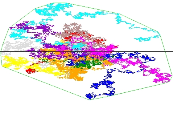
Figure 12: Convex hull of 10 open Brownian paths. (Paths are independent and start from the origin.)

Let us also make another observation. In the limit of large $n$, the prefactor for the average area of the convex hull of $n$ open Brownian paths, namely $\log n$, is identical not only to that of the average area of the convex hull of $n$ independent points drawn each from a Gaussian distribution $\rho(x,y)\propto e^{-\frac{x^{2}+y^{2}}{2}}$, but also to that of the number of distinct sites visited by $n$ independent random walkers on a lattice. Indeed the number of distinct sites visited by $n$ independent walkers on a lattice (eg $\mathbb{Z}^{2}$) has been studied systematically by H. Larralde et al. Larralde ; LarrNature (see also Yuste ). For $n$ lattice walks ($n\gg 1$) each of $k$ step (steps are only allowed to neighbourings sites), Larralde et al. have identified three regimes according to the value of $k$. For the second of these regimes, the intermediate one, the system is in a sort of diffusive state so that the number of distinct sites visited $\langle S_{n}(k)\rangle$ grows like the area of the disk of radius $\sqrt{k}$, that is, proportionally to $k$, with a prefactor $\log n$. In this regime, Acedo and Yuste Yuste describe the explored territory as ”a corona of dendritic nature [characterized by filaments created by the random walkers wandering in the outer regions] and an inner hyperspherical core [where there is much overlapping].” (cf. fig. 13).

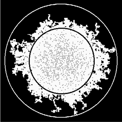
Figure 13: Figure from Acedo and Yuste Yuste : ”A snapshot of the set of sites visited by $n=1000$ random walkers on the two-dimensional lattice. The visited sites are in white, the unvisited ones are in black and the internal gray points are the random walkers. The outer white circle is centered on the starting point of the random walkers and its radius is the maximum distance from that point reached by any walker at the time the snapshot was taken. The internal black circle is concentric with the former but its radius is the distance between the origin and the nearest unvisited site.”

The detailed transposition between lattice-walk models and ours ($n$ planar Brownian motions of fixed duration $T$) requires much care, but it is interesting to note that in the intermediate regime, the number of distinct sites visited by $n$ independent lattice walkers grows like a circle with the same radius as that of the convex hull of $n$ planar Brownian paths.

6 Conclusion

The method presented in this paper, based on the use of support functions and Cauchy formulae, allows one to treat, in a general way, random convex hull problems in a plane, whether the random points considered are independent or correlated. Our work makes an important link between the two-dimensional convex hull problem and the subject of extreme value statistics.

We have shown here how this method can be implemented successfully in the case of independent points in the plane and when the points are correlated as in the case when the points represent the positions of a planar Brownian motion of a given fixed duration $T$. This method should be adaptable to treat other types of random paths, such as discrete-time random walks or anomalous diffusion processes such as Lévy flights.

In addition, we have shown how to suitably generalise this method to compute the mean perimeter and the mean area of the global convex hull of $n$ independent Brownian paths. Our work leads to several interesting open questions:

• For example, can one go beyond the first moment and compute, for instance, the full distribution of the perimeter and the area of the convex hull of $n$ independent Brownian paths?

• For a single random walker of $N$ steps, the average number of vertices of its convex hull is known from Baxter’s work Bax : $\langle F_{N}\rangle=2(1+1/2+1/3+\ldots+1/N)\sim 2\log(N)$ for large $N$. It remains an outstanding problem to generalise this result to the case of the convex hull of $n$ independent random walkers each of step $N$.

• Furthermore, we have only studied the convex hull of $n$ independent Brownian paths. However, in many situations, the animals interact with each other leading to collective behavior such as flocking. It would thus be very interesting to study the effect of interaction between walkers on the statistics of their convex hull.

• Finally, it would be interesting to study the statistics of the convex polytope associated with Brownian paths (one or more) in $3$ dimensions. Let us remark that Cauchy’s formula exist in higher dimensions and that it is possible to apply a method similar to the one developped here in order to compute the average surface area.

Appendix A Proof of Cauchy’s formulae

We give here a quick ”proof” of Cauchy’s formulae:

$$L=\int_{0}^{2\pi}M(\theta)\ d\theta$$ (169)

$$A=\frac{1}{2}\int_{0}^{2\pi}\left(M^{2}(\theta)-\left(M^{\prime}(\theta)\right)^{2}\right)\ d\theta$$ (170)

We consider a polygonal curve and, without loss of generality, examine the integrals appearing in Cauchy’s formulae on a portion of the curve corresponding to the configuration shown on figure A.

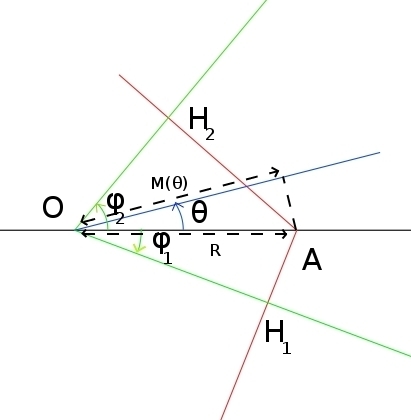
Figure 14: Portion of a polygonal curve (in red) near one of its vertices (A), with the lines through the origin perpendicular to the curve before A and after A (in green), together with the line of direction $\theta$ (in blue)

.

On the interval $\theta\in[-\phi_{1},\phi_{2}]$, the value of the support function of the polygonal curve will be given by $A$. Writing $R$ for the distance between the origin $O$ and vertex $A$, we therefore have:

$$M(\theta)=R\cos\theta$$ (171)

The first of Cauchy’s formulae then gives:

$$L=\int_{-\phi_{1}}^{\phi_{2}}\ M(\theta)\ d\theta=R(\sin\phi_{1}+\sin\phi_{2}),$$ (172)

which is indeed the length of the curve (that is, $H_{1}A+AH_{2}$) between $H_{1}$ and $H_{2}$.

As for the second of Cauchy’s formulae, it gives:

$$A =\frac{1}{2}\int_{-\phi_{1}}^{\phi_{2}}\ \left(\left[M(\theta)\right]^{2}-\left[M^{\prime}(\theta)\right]^{2}\right)\ d\theta$$

$$=\frac{R^{2}}{2}\int_{-\phi_{1}}^{\phi_{2}}\ \left[\cos^{2}\theta-\sin^{2}\theta\right]d\theta$$

$$=\frac{R^{2}}{2}\left(\sin\phi_{2}\ \cos\phi_{2}+\sin\phi_{1}\ \cos\phi_{1}\right)$$

which is indeed the area of the polygon $OH_{1}AH_{2}$.

This proves the formulae for closed polygonal curves containing the origin. If the origin is outside, one can see that the signs of the various terms will lead to cancellations and the formulae will remain valid. Finally, taking the continuous limit yields the result for smooth curves.

Appendix B Time at which the maximum of $n$ 1-dimensional Brownian motion is attained

Let us write:

$$\text{Prob}(M_{n}=M,\tau^{*}=\tau)\equiv\rho_{n}(\tau,M)\ d\tau\ dM,$$ (173)

where:

• $M_{n}$ is the global maximum of the $n$ Brownian motions,

• $\tau^{*}$ is the time at which this global maximum is attained,

• $\rho_{n}$ is the joint probability density function of $M_{n}$ and $\tau^{*}$.

This probability can be written as the probability that one of the motions attains its maximum $M$ at time $\tau$ and the $n-1$ others all have a maximum which is less than $M$:

$$\rho_{n}(\tau,M)=n\rho_{1}(\tau,M)[F(M)]^{n-1},$$ (174)

$F(M)$ being, as before, the cumulative distribution function of the maximum of one standard Brownian motion on the interval $[0,T]$:

$$F(M)=\text{erf}\left(\frac{M}{\sqrt{2T}}\right).$$

The joint probability density function $\rho_{1}(\tau,M)$ of the maximum $M$ and the time $\tau$ at which it happens can be computed using various techniques. The simplest of them is to use the Feynman-Kac path integral method, but suitably adapted with a cut-off SMAC ; SM . This technique has recently been used RFSM ; MKRF to compute exactly the joint distribution $\rho_{1}(\tau,M)$ of a single Brownian motion, but subject to a variety of constraints, such as for a Brownian excursion, a Brownian meander etc. The results are nontrivial MKRF and have been recently verified using an alternative functional renormalization group approach GSPL . For a single free Brownian motion (the case here), this method can be similarly used and it provides a simple and compact result

$$\rho_{1}(\tau,M)=\frac{M}{\pi\tau^{\frac{3}{2}}\sqrt{T-\tau}}e^{-\frac{M^{2}}{2\tau}}.$$

We then obtain the marginal distribution $\rho_{n}(\tau)$ by integrating out $M$. It has the scaling form $\rho_{n}(\tau)=\frac{1}{T}f_{n}\left(\frac{\tau}{T}\right)$ where the scaling function $f_{n}(z)$ is given in Eq. (148) and is plotted, for various values of $n$, in Fig. (9).

For Brownian bridges, the reasoning is exactly the same, but of course $F(M)$ and $\rho_{1}$ differ:

$$\rho_{1}(\tau,M) = \frac{2T}{\pi}\frac{M^{2}}{[\tau(T-\tau]\frac{3}{2}}\ e^{-\frac{M^{2}T}{2\tau(T-\tau)}}$$ (175)

$$F(M) = 1-e^{-\frac{2M^{2}}{T}},$$ (176)

which can both be derived using the technique we pointed to above ACSM1 ; SM ; RFSM ; MKRF .

We then obtain $\rho_{n}(\tau)=\frac{1}{T}g_{n}\left(\frac{\tau}{T}\right)$ where

$$g_{n}(z)=\frac{4n}{\sqrt{\pi}}\int_{0}^{\infty}\ u^{2}\ e^{-u^{2}}\ \left[1-e^{-4u^{2}\,z\,(1-z)}\right]^{n-1}\ du.$$ (177)

Figure 10 shows a plot of $g_{n}(z)$ for different values of $n$.

Appendix C Asymptotic behaviour

C.1 Open paths - average perimeter

Letting $M_{n}$ be the maximum of $n$ independent Brownian paths each of duration $T$, we write $\mathrm{Prob}(M_{n}\leq M)\equiv F_{n}(M)$. This can be expressed in terms of the cumulative distribution function $F_{1}(M)$ of the maximum of a standard one-dimensional Brownian motion:

$$F_{n}(M) = [F(M)]^{n}$$ (178)

$$= \left[\frac{2}{\sqrt{\pi}}\int_{0}^{\frac{M}{\sqrt{2T}}}\ e^{-u^{2}}\ du\right]^{n}$$

$$= \left[1-\frac{2}{\sqrt{\pi}}\int_{\frac{M}{\sqrt{2T}}}^{\infty}\ e^{-u^{2}}\ du\right]^{n}$$

In the limit when $n$ and $M$ become very large, (178) becomes:

$$F_{n}(M) \sim \exp\left[n\ln\left(1-\frac{2}{\sqrt{\pi}}\int_{\frac{M}{\sqrt{2T}}}^{\infty}\ e^{-u^{2}}\ du\right)\right]$$ (179)

$$\sim \exp\left[-n\frac{2}{\sqrt{\pi}}\int_{\frac{M}{\sqrt{2T}}}^{\infty}\ e^{-u^{2}}\ du\right]$$

Integrating by parts yields:

$$\int_{\frac{M}{\sqrt{2T}}}^{\infty}\ e^{-u^{2}}\ du=\frac{\sqrt{T}\,e^{-\frac{M^{2}}{2T}}}{\sqrt{2}M}+O(1)$$ (180)

Inserting this into equation (179), one obtains:

$$F_{n}(M) \sim e^{\frac{-2\,n\,\sqrt{T}\,e^{-M^{2}/2T}}{M\sqrt{2\pi}}}$$ (181)

$$\sim e^{-e^{-\frac{1}{2T}\left(M^{2}-2T\ln n\right)}}$$ (182)

Here we write:

$$\delta\equiv M-\sqrt{2T\ln n},$$

assuming that $\delta$ vanishes at large $n$, as we will be able to check a posteriori. It follows that:

$$M^{2}=2T\ln n\left(1+\frac{\delta}{\sqrt{2T\ln n}}\right)^{2}\sim 2T\ln n\left(1+\frac{2\delta}{\sqrt{2T\ln n}}\right)$$

Hence:

$$M^{2}-2T\ln n\sim 2\delta\sqrt{2T\ln n}=2\sqrt{2T\ln n}\left(M-\sqrt{2T\ln n}\right)$$

Inserting this into (182) yields:

$$F_{n}(M)\sim e^{-e^{-\sqrt{\frac{2\ln n}{T}}\left(M-\sqrt{2T\ln n}\right)}}$$ (183)

Now, to compute the asymptotic behaviour of $M_{n}$ when $n$ is large, let us start from:

$$\langle M_{n}\rangle = \int_{0}^{\infty}MF_{n}^{\prime}(M)\ dM$$ (184)

$$\sim \int_{A}^{\infty}MF_{n}^{\prime}(M)\ dM$$

where $A>>1$ will ”disappear” at a later stage.
Combining this with Eq. (183), one obtains:

$$\langle M_{n}\rangle\sim\int_{A}^{\infty}\ M\ \sqrt{\frac{2\ln n}{T}}e^{-\sqrt{\frac{2\ln n}{T}}\left(M-\sqrt{2T\ln n}\right)}e^{-e^{-\sqrt{\frac{2\log n}{T}}\left(M-\sqrt{2T\ln n}\right)}}\ dM$$ (185)

Setting:

$$y=\sqrt{\frac{2\log n}{T}}\left(M-\sqrt{2T\ln n}\right)$$

one arrives at:

$$\langle M_{n}\rangle\sim\int_{\sqrt{\frac{2\ln n}{T}}\left(A-\sqrt{2T\ln n}\right)}^{\infty}\ \left(\sqrt{2T\ln n}+y\sqrt{\frac{T}{2\ln n}}\right)\,e^{-y}\,e^{-e^{-y}}\ dy$$ (186)

In the limit when $n\rightarrow\infty$, this leads to:

$$\langle M_{n}\rangle \sim \int_{-\infty}^{\infty}\ \sqrt{2T\ln n}\,e^{-y}\,e^{-e^{-y}}\ dy$$ (187)

$$\sim \sqrt{2T\ln n}$$

Thus, the average perimeter of the convex hull of $n$ Brownian paths in the plane behaves for large $n$

$$\langle L_{n}\rangle \sim 2\pi\sqrt{2T\ln n}.$$ (188)

C.2 Open paths: average area

We wish to compute the asymptotical behaviour (for $n$ large) of the average area of the convex hull of $n$ open Brownian paths in the plane, all independent and of duration $T$. We apply Cauchy’s formula (139) in the context of isotropic samples:

$$\langle A_{n}\rangle=\pi\left(\langle M_{n}^{2}\rangle-\langle[M^{\prime}_{n}]^{2}\rangle\right).$$ (189)

The first term of the right-hand side is easily computed (it suffices to substitute $M^{2}$ for $M$ in Eq. (185)):

$$\langle M_{n}^{2}\rangle\sim 2T\ln n$$ (190)

To obtain (153), it thus remains to show that $\langle A_{n}\rangle$ is dominated by $\langle M_{n}^{2}\rangle$. Recall Eq. (149):

$$\langle A_{n}\rangle={4nT}\,{\sqrt{\pi}}\,\int_{0}^{\infty}du\ u\ \left[\text{erf}(u)\right]^{n-1}\left(ue^{-u^{2}}-g(u)\right),$$ (191)

where

$$g(u)=\frac{1}{2\sqrt{\pi}}\int_{0}^{1}\frac{e^{-{u^{2}}/{\tau}}\ dt}{\sqrt{\tau(1-\tau)}}.$$

The integral in Eq. (191) is dominated by the contribution from the large-$u$ part. Therefore, we examine in this limit:

$$\int_{0}^{1}d\tau\frac{1}{\sqrt{\tau(1-\tau)}}e^{-\frac{u^{2}}{\tau}}$$ (192)

Setting $\tau=1-y$:

$$\int_{0}^{1}d\tau\frac{1}{\sqrt{\tau(1-\tau)}}e^{-\frac{u^{2}}{\tau}} = \int_{0}^{1}\ dy\frac{1}{\sqrt{y(1-y)}}e^{-\frac{u^{2}}{1-y}}$$ (193)

$$\sim \int_{0}^{1}\ dy\frac{1}{\sqrt{y(1-y)}}e^{-u^{2}(1+y)}$$ (194)

$$\sim e^{-u^{2}}\int_{0}^{1}\ dy\frac{1}{\sqrt{y(1-y)}}e^{-yu^{2}}$$ (195)

We now write:

$$z=u\sqrt{y}.$$

This leads to:

$$\int_{0}^{1}d\tau\frac{1}{\sqrt{\tau(1-\tau)}}e^{-\frac{u^{2}}{\tau}} \sim e^{-u^{2}}\int_{0}^{u}\ \frac{2z\ dz}{u^{2}}\frac{1}{\sqrt{\frac{z^{2}}{u^{2}}(1-\frac{z^{2}}{u^{2}})}}e^{-z^{2}}$$

$$\sim \frac{2e^{-u^{2}}}{u}\int_{0}^{u}\ dz\frac{1}{\sqrt{1-\frac{z^{2}}{u^{2}}}}e^{-z^{2}}$$

$$\sim \frac{2e^{-u^{2}}}{u}\int_{0}^{u}\ dz(1+\frac{z^{2}}{2u^{2}})e^{-z^{2}}$$

$$\sim \frac{2e^{-u^{2}}}{u}\sqrt{\frac{\pi}{2}}\text{erf}(u)+\frac{e^{-u^{2}}}{u}\int_{0}^{x}\ dz\ \frac{z^{2}e^{-z^{2}}}{u^{2}}$$

An integration by parts shows that the second term on the right-hand side is $o\left(\frac{e^{-u^{2}}}{u^{2}}\right)$, whence:

$$\int_{0}^{1}d\tau\frac{1}{\sqrt{\tau(1-\tau)}}e^{-\frac{u^{2}}{\tau}}\sim\frac{\sqrt{\pi}e^{-u^{2}}}{u}.$$ (196)

Returning to Eq. (191), where the integral is dominated by the contribution from the large $u$ part, we have:

$$\langle A_{n}\rangle = {4nT}\,{\sqrt{\pi}}\,\int_{0}^{\infty}du\ u\ \left[\text{erf}(u)\right]^{n-1}\left(ue^{-u^{2}}-g(u)\right)$$ (197)

$$\sim {4nT}\,{\sqrt{\pi}}\,\int_{0}^{\infty}du\ u\ \left[\text{erf}(u)\right]^{n-1}\left(ue^{-u^{2}}-\frac{e^{-u^{2}}}{2u}\right)$$ (198)

$$\sim {4nT}\,{\sqrt{\pi}}\,\int_{0}^{\infty}du\ u^{2}\ \left[\text{erf}(u)\right]^{n-1}e^{-u^{2}}$$ (199)

$$\sim \pi\langle M_{n}^{2}\rangle$$ (200)

$$\sim 2\pi T\ln n.$$ (201)

C.3 Closed paths: average perimeter

The calculation is analogous to that of subsection C.1; indeed, the only difference is that the cumulative distribution function $F_{n}$ of the maximum $M$ of $n$ one-dimensional Brownian bridges is given by:

$$F_{n}(M)=[1-e^{-\frac{2M^{2}}{T}}]^{n}$$ (202)

In the limit when $n$ and $M$ become very large, we then have:

$$F_{n}(M) \sim \exp\left[n\ln\left(1-e^{-\frac{2M^{2}}{T}}\right)\right]$$ (203)

$$\sim e^{-e^{-\frac{2}{T}\left(M^{2}-\frac{T}{2}\ln n\right)}}$$

We retrieve here the same equation as (182), where $T$ is replaced by $\frac{T}{4}$. We can thus deduce the result given in (160):

$$\langle L_{n}\rangle \sim \pi\sqrt{2T\ln n}.$$ (204)

C.4 Closed paths: average area

We wish to compute the asymptotic behaviour (for $n$ large) of the average area of the convex hull of $n$ closed Brownian paths in the plane, all independent and of duration $T$. The analysis is similar to that of subsection C.2. We apply Cauchy’s formula (139) in the context of isotropic samples:

$$\langle A_{n}\rangle=\pi\left(\langle M_{n}^{2}\rangle-\langle[M^{\prime}_{n}]^{2}\rangle\right).$$ (205)

The first term on the right-hand side is, as before, easily computed from subsections C.3 and C.1:

$$\langle M_{n}^{2}\rangle\sim\frac{T}{2}\ln n$$ (206)

We now show that $\langle A_{n}\rangle$ is dominated by $\langle M_{n}^{2}\rangle$. The equivalent of Eq. (191) for closed paths is:

$$\langle A_{n}\rangle=\frac{2nT}{\sqrt{\pi}}\ \int_{0}^{\infty}\ du\ u^{2}\left(1-e^{-u^{2}}\right)^{n-1}\left(ue^{-u^{2}}-g(u)\right),$$ (207)

where:

$$g(u)=\frac{1}{8}\int_{0}^{1}\ d\tau\ \frac{e^{-\frac{u^{2}}{4\tau(1-\tau)}}}{\sqrt{\tau(1-\tau)}}.$$

The integral in Eq. (207) is dominated by the contribution from the large-$u$ part. Therefore, we examine $g(u)$ in this limit.

$$g(u) = \frac{1}{8}\int_{0}^{1}\ d\tau\ \frac{e^{-\frac{u^{2}}{4\tau(1-\tau)}}}{\sqrt{\tau(1-\tau)}}$$ (208)

$$= \frac{1}{4}\int_{0}^{\frac{1}{2}}\ d\tau\ \frac{e^{-\frac{u^{2}}{4\tau(1-\tau)}}}{\sqrt{\tau(1-\tau)}}$$ (209)

We now write:

$$\tau=\frac{1}{2}-z.$$

This leads to:

$$\frac{1}{4}\int_{0}^{\frac{1}{2}}\ d\tau\ \frac{e^{-\frac{u^{2}}{4\tau(1-\tau)}}}{\sqrt{\tau(1-\tau)}} = \frac{1}{2}\int_{0}^{\frac{1}{2}}\ dz\ \frac{e^{-\frac{u^{2}}{1-4z^{2}}}}{\sqrt{1-4z^{2}}}$$

Setting:

$$v=2uz,$$

then yields:

$$\frac{1}{2}\int_{0}^{\frac{1}{2}}\ dz\ \frac{e^{-\frac{u^{2}}{1-4z^{2}}}}{\sqrt{1-4z^{2}}} = \frac{1}{4}\int_{0}^{u}\ \frac{dv}{u}\ \frac{e^{-\frac{u^{2}}{1-\frac{v^{2}}{u^{2}}}}}{\sqrt{1-\frac{v^{2}}{u^{2}}}}$$

$$\sim \frac{1}{4}\frac{e^{-u^{2}}}{u}\int_{0}^{u}\ dv\ e^{-v^{2}}(1+\frac{v^{2}}{2u^{2}})$$

$$\sim \frac{e^{-u^{2}}}{8u}\sqrt{\pi}\ \text{erf}(u)+O\left(\frac{e^{-u^{2}}}{u^{2}}\right)$$

Returning to Eq. (207), where the integral is dominated by the contribution from the large-$u$ part, we therefore have:

$$\langle A_{n}\rangle = \frac{2nT}{\sqrt{\pi}}\ \int_{0}^{\infty}\ du\ u^{2}\left(1-e^{-u^{2}}\right)^{n-1}\left(ue^{-u^{2}}-g(u)\right)$$ (210)

$$\sim \frac{2nT}{\sqrt{\pi}}\ \int_{0}^{\infty}\ du\ u^{2}\left(1-e^{-u^{2}}\right)^{n-1}\left(ue^{-u^{2}}-\frac{\sqrt{\pi}e^{-u^{2}}}{8u}\right)$$ (211)

$$\sim \frac{2nT}{\sqrt{\pi}}\ \int_{0}^{\infty}\ du\ u^{3}\left(1-e^{-u^{2}}\right)^{n-1}e^{-u^{2}}$$ (212)

$$\sim \pi\langle M_{n}^{2}\rangle$$ (213)

$$\sim \frac{\pi T}{2}\ln n.$$ (214)

References

- (1) Abramowitz, M., Stegun, I.: Handbook of Mathematical Functions with Formulas, Graphs, and Mathematical Tables. Dover (1964)
- (2) Acedo, L., Yuste, S.B.: Multiparticle random walks. Recent Res. Dev. Stat. Phys. 2, 83–106 (2002)
- (3) Affentranger, F.: The expected volume of a random polytope in a ball. Journal of Microscopy 151, 277–287 (1988)
- (4) Agrawal, H., Dhar, D.: Probability distribution of the sizes of largest erased-loops in loop-erased random walks. Phys. Rev. E 65(031108) (2002)
- (5) Akl, S., Toussaint, G.: Efficient convex hull algorithms for pattern recognition applications. In: International Conference on Pattern Recognition, pp. 483–487 (1978)
- (6) Aldous, D., Fristedt, B., Griffin, P.S., Pruitt, W.E.: The number of extreme points in the convex hull of a random sample. J. Appl. Prob. 28, 287–304 (1991)
- (7) Ayari, S., Dubuc, S.: La formule de Cauchy sur la longueur d’une courbe. Canad. Math. Bull. 40, 3–9 (1997)
- (8) Bárány, I.: Stochastic Geometry. C.I.M.E., Lecture Notes Math. 1892. Springer (2006)
- (9) Bárány, I., Reitzner, M.: Random polytopes. preprint (www.renyi.hu/ barany/cikkek/clt-pol2.pdf) (2008)
- (10) Bárány, I., Vu, V.: Central limit theorems for Gaussian polytopes. Ann. Prob. 35(4), 1593–1621 (2007)
- (11) Barbier, E.: Note sur le problème de l’aiguille et le jeu du joint couvert. J. Math. Pures Appl. 5, 273–286 (1860)
- (12) Bartumeus, F., da Luz, M., Viswanathan, G., Catalan, J.: Animal search strategies: A quantitative random-walk analysis. Ecology (2005)
- (13) Baxter, G.: A combinatorial lemma for complex numbers. Ann. Math. Stat. 32(3), 901 (1961)
- (14) Ben Naim, E., Krapivsky, P.L., Majumdar, S.N.: Extremal properties of random trees. Phys. Rev. E. 64(R035101) (2001)
- (15) Bena, I., Majumdar, S.N.: Universal extremal statistics in a freely expanding jepsen gas. Phys. Rev. E 75(051103) (2007)
- (16) Berg, H.: Random Walks in Biology. Princeton University Press, New York (1983)
- (17) Bhattacharya, B., Sen, S.: On a simple, practical, optimal, output-sensitive randomized planar convex hull algorithm. Journal of Algorithms 25, 173–193 (1997)
- (18) Biane, P., Letac, G.: The mean perimeter of some random plane convex sets generated by a Brownian motion. Preprint (2009). ArXiv:0905.2256
- (19) Biroli, G., Bouchaud, J.P., Potters, M.: Extreme value problems in random matrix theory and other disordered systems. JSTAT (P07019) (2007)
- (20) Bouchaud, J.P., Mézard, M.: Universality classes for extreme value statistics. J. Phys. A.: Math. Gen. 30, 7997–8015 (1997)
- (21) Boyle, S., Lourenço, W., da Silva, L., Smith, A.: Home-range estimates vary with sample size and methods. Folia Primatologica 80, 33–42 (2009)
- (22) Bräker, H., Hsing, T.: On the area and perimeter of a random convex hull in a bounded convex set. Prob. Theory Relat. Fields pp. 517–550 (1998)
- (23) Bramson, M.: Maximal displacement of branching brownian motion. Comm. Pure Appl. Math. 31, 531–581 (1978)
- (24) Brown, B., Resnick, S.I.: Extreme values of independent stochastic processes. J. Appl. Prob. 14(4), 732–739 (1977)
- (25) Brozius, H.: Convergence in mean of some characteristics of the convex hull. Adv. Appl. Prob. 21, 526–542 (1989)
- (26) Brozius, H., de Haan, J.: On limiting laws for the convex hull of a sample. J. Appl. Prob. 24, 852 (1987)
- (27) Brunet, E., Derrida, B.: Statistics at the tip of a branching random walk and the delay of traveling waves. Europhys. Lett. 87(60010) (2009)
- (28) Buchta, C.: Zufallspolygone in konvexen Vielecken. J. reine u. angew. Math. 347, 212–220 (1983)
- (29) Buchta, C.: Zufällige Polyeder. Lecture Notes in Mathematics 114, Springer (1985)
- (30) Burdzy, K.: Brownian motion in cones. Ann. Prob. 13, 1006–1010 (1985)
- (31) Burdzy, K., San Martin, J.: Curvature of the convex hull of planar Brownian motion near its minimum point. Stoch. Process. Appl. 33(1), 89–103 (1989)
- (32) Burkhardt, T.W., Gyorgi, G., Moloney, N.R., Racz, Z.: Extreme statistics for time series: Distribution of the maximum relative to the initial value. Phys. Rev. E 76(041119) (2007)
- (33) Cabo, J., Groeneboom, P.: Limit theorems for functionals of convex hulls. Prob. Theory Relat. Fields 100, 31–55 (1994)
- (34) Calka, P., Schreiber, T.: Large deviation probabilities for the number of vertices of random polytopes in the ball. Adv. Appl. Prob. 38, 47–58 (2006)
- (35) Carnal, H.: Die konvexe hülle von rotationssymmetrischverteilen punkten. Z. Wahrsch. 15, 168–176 (1970)
- (36) Carpentier, D., LeDoussal, P.: Glass transition of a particle in a random potential, front selection in nonlinear renormalization group, and entropic phenomena in liouville and sinh-gordon models. Phys. Rev. E 63(026110) (2001)
- (37) Cauchy, A.: La rectification des courbes. Mémoire de l’Académie des Sciences (1832)
- (38) Chassaing, P., Marckert, J.F., Yor, M.: A stochastically quasi-optimal search algorithm for the maximum of the simple random walk. Ann. Appl. Prob. 13(4), 1264–1295 (2003)
- (39) Coffman, E.G., Flajolet, P., Flato, L., Hofro, M.: The maximum of random walk and its application to rectangle packing. Prob. in Eng. and Inform. Sciences 12, 373–386 (1998)
- (40) Coles, S.: An Introduction to Statistical Modeling of Extreme Values. Springer Series in Statistics. Springer Verlag, London (2001)
- (41) Comtet, A., Majumdar, S.N.: Precise asymptotics of a random walker’s maximum. J. Stat. Mech. (P06013) (2005)
- (42) Cranston, M., Hsu, P., March, P.: Smoothness of the convex hull of planar Brownian motion. Annals Prob 17(1), 144 (1989)
- (43) Crofton, M.: On the theory of local probability, applied to straight lines at random in a plane. Trans. Roy. Soc. 158, 181–199 (1868)
- (44) Daniels, H.E., Skyrme, T.H.R.: The maximum of a random walk whose mean path has a maximum. Adv. Appl; Prob. 17(1), 85–99 (1985)
- (45) Davis, R., Mulrow, E., Resnick, S.: The convex hull of a random sample in . Comm. Statist. Stoch. Models 3(1), 1–27 (1987)
- (46) Dean, D.S., Majumdar, S.N.: Extreme-value statistics of hierarchically correlated variables, deviation from gumbel statistics and anomalous persistence. Phys. Rev. E 64(046121) (2001)
- (47) Dean, D.S., Majumdar, S.N.: Large deviations of extreme eigenvalues of random matrices. Phys. Rev. Lett. 97(160201) (2006)
- (48) Dean, D.S., Majumdar, S.N.: Extreme value statistics of eigenvalues of gaussian random matrices. Phys. Rev. E 77(041108) (2008)
- (49) Derrida, B.: Random-energy model - an exactly solvable model of disordered-systems. Phys. Rev. B 24, 2613–2626 (1981)
- (50) Derrida, B., Spohn, H.: Polymers on disordered trees, spin glasses, and travelling waves. J. Stat. Phys. 51, 817–840 (1988)
- (51) Devroye, L.: How to reduce the average complexity of convex hull finding algorithms. Comp. Math. Appl. 7, 299–308 (1981)
- (52) Dobrushin, R.L., Kotecký, R., Shlosman, S.: Wulff construction: a global shape from local interaction. Translations of Mathematical Monographs. American Mathematical Society, Providence, Rhode Island (1992)
- (53) Eddy, W.: A new convex hull algorithm for planar sets. ACM Trans. Math. Software 3(4), 398–403 (1977)
- (54) Eddy, W.: The distribution of the convex hull of a Gaussian sample. J. Appl. Prob. 17, 686–695 (1980)
- (55) Eddy, W., Gale, J.: The convex hull of a spherically symmetric sample. Adv. Appl. Prob. 13, 751–763 (1981)
- (56) Edelstein-Keshet, L.: Mathematical Models in Biology. Random House, New York (1988)
- (57) Efron, B.: The convex hull of a random set of points. Biometrika 52(3 and 4), 331 (1965)
- (58) El Bachir, M.: L’enveloppe convexe du mouvement brownien. Ph.D. thesis, Université Paul Sabatier, Toulouse, France (1983)
- (59) Evans, M.R., Majumdar, S.N.: Condensation and extreme value statistics. JSTAT (P05004) (2008)
- (60) Evans, S.N.: On the Hausdorff dimension of Brownian cone points. Math. Proc. Camb. Philos. Soc. 98, 343–353 (1985)
- (61) Feller, W.: An Introduction to Probability Theory and its Applications. Wiley, New York (1968)
- (62) Finch, S., Hueter, I.: Random convex hulls: a variance revisited. Adv. Appl. Prob. 36(4), 981–986 (1994)
- (63) Fyodorov, Y.V., Bouchaud, J.P.: Freezing and extreme value statistics in a random energy model with logarithmically correlated potential. J. Phys. A.: Math. Theor. 41(372001) (2008)
- (64) Fyodorov, Y.V., LeDoussal, P., Rosso, A.: Statistical mechanics of logarithmic rem: duality, freezing and extreme value statistics of 1/f noises generated by gaussian free fields. JSTAT (P10005) (2009)
- (65) Garcia-Garcia, R., Rosso, A., Schehr, G.: The longest excursion of fractional brownian motion : numerical evidence of non-markovian effects. arXiv:0911:1897 (2009)
- (66) Geffroy, J.: Contribution à la théorie des valeurs extrêmes. II. Publ. Inst. Stat. Univ. Paris 7(8), 3–65 (1959)
- (67) Geffroy, J.: Localisation asymptotique du polyèdre d’appui d’un échantillon Laplacien à dimensions. Publ. Inst. Stat. Univ. Paris 10, 213–228 (1961)
- (68) Giuggioli, L., Abramson, G., Kenkre, V.M., Parmenter, R.R., Yates, T.L.: Theory of home range estimation from displacement measurements of animal populations. J. Theor. Biol. 240, 126–135 (2006)
- (69) Gnedenko, B.: Sur la distribution limite du terme maximum d’une série aléatoire. Ann. Math. 44(3), 423–453 (1943)
- (70) Godrèche, C., Luck, J.M.: A record-driven growth process. JSTAT (P11006) (2008)
- (71) Godrèche, C., Majumdar, S.N., Schehr, G.: The longest excursion of stochastic processes in nonequilibrium systems. Phys. Rev. Lett. 102(240602) (2009)
- (72) Goldman, A.: Le spectre de certaines mosaïques poissoniennes du plan et l’enveloppe convexe du pont brownien. Prob. Theor. Relat. Fields 105, 57–83 (1996)
- (73) Goldman, A.: Sur une conjecture de D.G. Kendall concernant la cellule de Crofton du plan et sur sa contrepartie brownienne. C.R. Acad. Sc. Paris 326, 233–237 (1998)
- (74) Graham, R.: An efficient algorithm for determining the convex hull of a finite planar set. Information Processing Letters 1, 132,133 (1972)
- (75) Groeneboom, P.: Limit theorems for convex hulls. Prob. Theory Relat. Fields 79, 327–368 (1988)
- (76) Gumbel, E.: Les valeurs extrêmes des distributions statistiques. Annales de l’I.H.P. 5(2), 115–158 (1935)
- (77) Gumbel, E.: Statistics of Extremes. Columbia University Press, New York (1958)
- (78) Gyorgi, G., Holdsworth, P.C.W., Portelli, B., Racz, Z.: Statistics of extremal intensities for gaussian interfaces. Phys. Rev. E 68(056116) (2003)
- (79) Gyorgi, G., Moloney, N.R., Ozogany, K., Racz, Z.: Maximal height statistics for signals. Phys. Rev. E 75(021123) (2007)
- (80) Haushofer, J., Bake, C.I., Livingstone, M.S., Kanwisher, N.: Privileged coding of convex shapes in human object-selective cortex. Journal of Neurophysiology 100, 753–762 (2008)
- (81) Hilhorst, H.J., Calka, P., Schehr, G.: Sylvester’s question and the random acceleration process. J. Stat. Mech.: Theory and Exp. (2008). P10010
- (82) Hsing, T.: On the asymptotic distribution of the area outside a random convex hull in a disk. Ann. Appl. Prob. 4, 478–493 (1994)
- (83) Jarvis, R.A.: On the identification of the convex hull of a finite set of points in the plane. Information Processing Letters 2, 18–21 (1973)
- (84) Jewell, N., Romano, J.: Coverage problems and random convex hulls. J. Applied Proba. 19, 546 (1982)
- (85) Johansson, K.: Shape fluctuations and random matrices. Commun. Math. Phys. 209, 437–476 (2000)
- (86) Kearney, M.J., Majumdar, S.N.: On the area under a continuous time Brownian motion till its first-passage time. J. Phys. A: Math. Gen. 38, 4097–4104 (2005)
- (87) Khoshnevisan, D.: Moment Inequalities for Functionals of the Brownian Convex Hull. Annals Prob. 20(2), 627 (1992)
- (88) Kirkpatrick, D.G., Seidel, R.: The ultimate planar convex hull algorithm? SIAM Journal on Computing 15(1), 287–299 (1986)
- (89) Krapivsky, P.L., Majumdar, S.N.: Traveling waves, front selection, and exact nontrivial exponents in a random fragmentation problem. Phys. Rev. Lett. 85, 5492 (2000)
- (90) Krug, J.: Records in a changing world. JSTAT (P07001) (2007)
- (91) Krug, J., Jain, K.: Breaking records in a evolutionary race. Physica A 358, 1–9 (2005)
- (92) Lakshminarayan, A., Tomsovic, S., Bohigas, O., Majumdar, S.N.: Extreme statistics of complex random and quantum chaotic states. Phys. Rev. Lett. 100(044103) (2008)
- (93) Larralde, H., Trunfio, P., Havlin, S., Stanley, H.E., Weiss, G.H.: Number of distinct sites visited by random walkers. Phys. Rev. A 45(10), 7128–7139 (1992)
- (94) Larralde, H., Trunfio, P., Havlin, S., Stanley, H.E., Weiss, G.H.: Territory Covered by Diffusing Particles. Nature 355, 423–426 (1992)
- (95) Le Gall, J.F.: Mouvement brownien, cônes et processus stables. Prob. Theory Relat. Fields 76, 587–627 (1987)
- (96) LeDoussal, P., Monthus, C.: Exact solutions for the statistics of extrema of some random landscapes, applications to the equilibrium and the dynamics of the toy model. Physica A 317, 140–198 (2003)
- (97) LeDoussal, P., Wiese, K.J.: Driven particle in a random landscape: disorder correlator, avalanche distribution and extreme value statistics of records. Phys. Rev. E 79(051105) (2009)
- (98) Letac, G.: Expected perimeter length. American Mathematical Monthly 85, 686 (1978)
- (99) Letac, G.: An explicit calculation of the mean of the perimeter of the convex hull of a plane random walk. J. Theor. Prob 6(2), 385 (1993)
- (100) Lévy, P.: Sur certains processus stochastiques homogènes. Comp. Math. 7, 283–339 (1939)
- (101) Lévy, P.: Processus stochastiques et mouvement brownien. Gauthiers-Villars, Paris (1948)
- (102) Lévy, P.: Le caractère universel de la courbe du mouvement brownien et la loi du logarithme itéré. Circ. Mat. Palermo Ser. 2.4, 337–366 (1955)
- (103) Majumdar, S.N.: Brownian functionals in Physics and Computer Science. Current Science 89, 2075 (2005)
- (104) Majumdar, S.N., Bohigas, O., Lakshminarayan, A.: Exact minimum eigenvalue distribution of an entangled random pure state. J. Stat. Phys. 131, 33–49 (2008)
- (105) Majumdar, S.N., Comtet, A.: Exact maximal height distribution of fluctuating interfaces. Phys. Rev. Letters 92(225501) (2004)
- (106) Majumdar, S.N., Comtet, A.: Airy distribution function: from the area under a Brownian excursion to the maximal height of fluctuating interfaces. J. Stat. Phys. 119, 777–826 (2005)
- (107) Majumdar, S.N., Comtet, A., Ziff, R.M.: Unified solution of the expected maximum of a random walk and the discrete flux to a spherical trap. J. Stat. Phys. 122, 833–856 (2006)
- (108) Majumdar, S.N., Krapivsky, P.L.: Extremal paths on a random cayley tree. Phys. Rev. E. 62, 7735 (2000)
- (109) Majumdar, S.N., Krapivsky, P.L.: Extreme value statistics and traveling fronts: An application to computer science. Phys. Rev. E. 65(036127) (2002)
- (110) Majumdar, S.N., Krapivsky, P.L.: Extreme value statistics and traveling fronts: various applications. Physica A: Statistical Mechanics and its Applications 318(1-2), 161–170 (2003)
- (111) Majumdar, S.N., Mallick, K., Sabhapandit, S.: Statistical properties of the final state in one-dimensional ballistic aggregation. Phys. Rev. E 79(021109) (2009)
- (112) Majumdar, S.N., Nechaev, S.K.: Exact asymptotic results for the bernoulli matching model of sequence alignment. Phys. Rev. E 72(020901) (2005)
- (113) Majumdar, S.N., Randon-Furling, J., Kearney, M.J., Yor, M.: On the time to reach maximum for a variety of constrained Brownian motions. J. Phys. A: Math. Theor. 41(365005) (2008)
- (114) Majumdar, S.N., Vergassola, M.: Large deviations of the maximum eigenvalue for wishart and gaussian random matrices. Phys. Rev. Lett. 102(060601) (2009)
- (115) Majumdar, S.N., Ziff, R.M.: Universal record statistics of random walks and levy flights. Phys. Rev. Lett. 101(050601) (2008)
- (116) McKean, H.P.: Application of brownian motion to the equation of kolmogorov-petrovskii-piskunov. Comm. Pure Appl. Math. 28, 323–331 (1976)
- (117) Meier, R., Ackermann, F., Herrmann, G., Posch, S., Sagerer, G.: Segmentation of molecular surfaces based on their convex hull. In: International Conference on Image Processing (ICIP’95), vol. 3, p. 3552 (1995)
- (118) Murphy, D., Noon, B.: Integrating Scientific Methods with Habitat Conservation Planning: Reserve Design for Northern Spotted Owls. Ecological Application 2, 3–17 (1992)
- (119) Nadal, C., Majumdar, S.N.: Non-intersecting Brownian interfaces and Wishart random matrices. Phys. Rev. E 79(061117) (2009)
- (120) Odlyzko, A.M.: Search for the maximum of a random walk. Random Structures Algorithms 6(275–295) (1995)
- (121) Preparata, F.P., Hong, S.J.: Convex hulls of finite sets of points in two and three dimensions. Communications of the ACM 20(2), 87–93 (1977)
- (122) Rambeau, J., Schehr, G.: Maximum relative height of one-dimensional interfaces: from rayleigh to airy distribution. JSTAT (P09004) (2009)
- (123) Randon-Furling, J., Majumdar, S.N.: Distribution of the time at which the deviation of a Brownian motion is maximum before its first-passage time. J. Stat. Mech. (P10008) (2007)
- (124) Randon-Furling, J., Majumdar, S.N., Comtet, A.: Convex Hull of Planar Brownian Motions: Exact results and an application to Ecology. Phys. Rev. Lett. 103(140602) (2009)
- (125) Raychaudhuri, S., Cranston, M., Przybyla, C., Shapir, Y.: Maximal height scaling of kinetically growing surfaces. Phys. Rev. Lett. 87(136101) (2001)
- (126) Raynaud, H.: Sur le comportement asymptotique de l’enveloppe convexe d’un nuage de points tirés au hasard dans . C. R. Acad. Sciences 261, 627–629 (1965)
- (127) Raynaud, H.: Sur l’enveloppe convexe des nuages de points aléatoires dans . J. Appl. Prob . 7(1), 35–48 (1970)
- (128) Reitzner, M.: Random polytopes and the Efron-Stein jackknife inequality. Ann. Prob. 31, 2136–2166 (2003)
- (129) Reitzner, M.: Central limit theorems for random polytopes. Prob. theory Relat. Fields 133, 483–507 (2005)
- (130) Reitzner, M.: The combinatorial structure of random polytopes. Adv. Math. 191, 178–208 (2005)
- (131) Rényi, A., Sulanke, R.: Über die konvexe Hülle von zufällig gewählten Punkten. Z. Wahrsch. 2, 75–84 (1963)
- (132) Rényi, A., Sulanke, R.: Über die konvexe Hülle von zufällig gewählten Punkten. Z. Wahrsch. 3, 138–147 (1964)
- (133) Rossing, T.D. (ed.): Handbook of acoustics. Springer (2007)
- (134) Sabhapandit, S.: Statistical properties of a single-file diffusion front. J. Stat. Mech. (L05002) (2007)
- (135) Sabhapandit, S., Majumdar, S.N.: Density of near-extreme events. Phys. Rev. Lett. 98(140201) (2007)
- (136) Sabhapandit, S., Majumdar, S.N., Redner, S.: Crowding at the front of marathon packs. J. Stat. Mech. (L03001) (2008)
- (137) Santaló, L.: Integral Geometry and Geometric Probability. Encyclopedia of Mathematics and Its Applications. Addison-Wesley (1976)
- (138) Schehr, G., LeDoussal, P.: Extreme value statistics from the real space renormalization group: Brownian motion, bessel processes and continuous time random walks. arXiv:0910:4913 (2009)
- (139) Schehr, G., Majumdar, S.N.: Universal asymptotic statistics of maximal relative height in one-dimensional solid-on-solid models. Phys. Rev. E 73(056103) (2006)
- (140) Schehr, G., Majumdar, S.N., Comtet, A., Randon-Furling, J.: Exact distribution of the maximal height of vicious walkers. Phys. Rev. Lett. 101(150601) (2008)
- (141) Schneider, R.: Random approximation of convex sets. Journal of Microscopy 151, 211 (1988)
- (142) Seidel, R.: Convex hull computations. In: J.E. Goodman, J. O’Rourke (eds.) Handbook of Discrete and Computational Geometry, pp. 361–375. CRC Press (1997)
- (143) Shimura, M.: A limit theorem for conditional random walk. Nagoya Math. J. 95, 105–116 (1984)
- (144) Shimura, M.: Excursions in a cone for two-dimensional Brownian motion. J. Math. Kyoto Univ. 13, 433–443 (1985)
- (145) Sirakov, N.M.: A new active convex hull model for image regions. J. Math. Imaging Vis. 26(3), 309–325 (2006)
- (146) Sire, C.: Probability distribution of the maximum of a smooth temporal signal. Phys. Rev. Lett. 98(020601) (2007)
- (147) Sire, C.: Contest based on a directed polymer in a random medium. Phys. Rev. E 78(061106) (2008)
- (148) Sire, C., Majumdar, S.N., Dean, D.S.: Exact solution of a model of time-dependent evolutionary dynamics in a rugged fitness landscape. JSTAT (L07001) (2006)
- (149) Snyder, T., Steele, J.: Convex hulls of random walks. Proc. Am. Math. Soc. 117(4), 1165 (1993)
- (150) Spitzer, F., Widom, H.: The circumference of a convex polygon. Proc. Am. Math. Soc. 12, 506–509 (1961)
- (151) Takács, L.: Expected perimeter length. Amer. Math. Month. 87, 142 (1980)
- (152) Toussaint, G.: A historical note on convex hull finding algorithms. Pattern Recognition Letters 3, 21–28 (1985)
- (153) Tracy, C., Widom, H.: Level-spacing distributions and the airy kernel. Commun. Math. Phys. 159, 151–174 (1994)
- (154) Valentine, F.: Convex sets. McGraw-Hill (1964)
- (155) Vivo, P., Majumdar, S.N., Bohigas, O.: Large deviations of the maximum eigenvalue in wishart random matrices. J. Phys. A: Math. Theor. 40, 4317–4337 (2007)
- (156) Vu, V.: Central limit theorems for random polytopes in a smooth convex set. Adv. Math 207, 221–243 (2006)
- (157) Weil, W., Wieacker, J.A.: Handbook of Convex Geometry, vol. B, pp. 1391–1438. North Holland (1993)
- (158) Wenger, R.: Randomized quick hull. Algorithmica 17, 322–329 (1997)
- (159) Worton, B.J.: A convex hull-based estimator of home-range size. Biometrics 51(4), 1206–1215 (1995)
- (160) Yaacoub, F., Hamam, Y., Abche, A., Fares, C.: Convex hull in medical simulations: a new hybrid approach. In: 32nd Annual Conference of IEEE Industrial Electronics Society, IECON’06, pp. 3308–3313 (2006)