Reduced Complexity Angle-Doppler-Range Estimation for MIMO Radar That Employs Compressive Sensing

Abstract

The authors recently proposed a MIMO radar system that is implemented by a small wireless network. By applying compressive sensing (CS) at the receive nodes, the MIMO radar super-resolution can be achieved with far fewer observations than conventional approaches. This previous work considered the estimation of direction of arrival and Doppler. Since the targets are sparse in the angle-velocity space, target information can be extracted by solving an $\ell_{1}$ minimization problem. In this paper, the range information is exploited by introducing step frequency to MIMO radar with CS. The proposed approach is able to achieve high range resolution and also improve the ambiguous velocity. However, joint angle-Doppler-range estimation requires discretization of the angle-Doppler-range space which causes a sharp rise in the computational burden of the $\ell_{1}$ minimization problem. To maintain an acceptable complexity, a technique is proposed to successively estimate angle, Doppler and range in a decoupled fashion. The proposed approach can significantly reduce the complexity without sacrificing performance.

I Introduction

Multiple-input multiple-output (MIMO) radar systems have received considerable attention in recent years. Unlike a phased-array radar, a MIMO radar [1] transmits multiple independent waveforms from its antennas. MIMO radar with widely separated antennas [2] exhibits spatial diversity, which improves target resolution. In colocated MIMO radar [3], phase differences induced by transmit and receive antennas can be exploited to form a long virtual array and thus achieve superior spatial resolution as compared to traditional radar systems. Compressive sensing (CS) is a recent development [4]-[5] and has already been applied successfully in diverse fields such as image processing and wireless communications. CS theory states that a $K$-sparse signal $\mathbf{x}$ of length $N$ can be recovered exactly with high probability from $\mathcal{O}(K\log N)$ measurements via $\ell_{1}$-optimization.

The application of CS to radar systems was investigated in [6]-[8], and to MIMO radar in [9]-[11]. In [10], a uniform linear array was considered as a transmit and receive antenna configuration. In [9] and [11], the authors proposed a MIMO radar implemented by a small scale network. According to [11], spatially distributed network nodes, each equipped with a single antenna, serve as transmit and receive antenna elements. The transmit nodes transmit periodic pulses. The receive nodes forward their compressive measurements to a fusion center. Exploiting the spareness of targets in the angle-Doppler space, an $\ell_{1}$-optimization problem is formulated and solved at the fusion center in order to extract target angle and Doppler information. This approach achieves the superior resolution of MIMO radar with far fewer samples than are required by conventional approaches. This implies low power consumption for the receive nodes.

The contribution of this paper is a low complexity CS approach for obtaining range as well as direction of arrival (DOA) and Doppler information about the target. Range estimation cannot not be obtained with the method of [11], as the target range causes an identical phase shift to the signals received at all nodes and during all pulses. One way to obtain range information is to measure the travel time of the emitted radar signal [10]. However, the range resolution of such an approach might be limited. In this paper, we modify the transmitted waveforms of the scheme of [11], so that range information is reflected in different phase shifts over different pulses. In particular, the transmit nodes transmit pulses whose frequency increases by some step from one pulse to the next. In this way, we introduce the step frequency radar approach [12] to MIMO radar, an approach that results in high range resolution. Range resolution tends to increase as the transmitted signal bandwidth increases. However, wideband signals correspond to very short pulses, which experience low signal-to-noise ratios at the receiver. A step frequency radar transmits a sequence of longer pulses that are narrowband and together cover a wide frequency range. Thus, a step frequency radar transmits an effectively wideband signal that does not suffer from low SNR problems. An extension of [11] to joint angle-Doppler-range estimation would be straightforward; however, it would involve prohibitively high complexity. In this paper, we propose an approach to obtain angle-Doppler-range information in a decoupled fashion, which results in significant complexity reduction. In [13], a decoupled angle-Doppler estimation approach was proposed for the case of slowly moving targets. In that case, we can assume that the Doppler shift varies between pulses but within each pulse remains approximately constant. Based on compressively collected observations during one pulse, one can obtain initial estimates of the azimuth angles by discretizing the angle space only. Then, Doppler information is extracted by combining the data of multiple pulses. The basis matrix requires a discretization of the Doppler space only for the initial angle estimates. In this paper, we apply a similar idea to decouple the estimation of angle, Doppler and range. We propose to transmit a pulse train with constant carrier frequency, followed by a pulse train with carrier frequency that varies between pulses. Based on the received data during the first pulse train one can decouple angle and Doppler estimation along the lines of [13]. Based on these initial angle-Doppler estimates, the range information can be extracted from the data corresponding to pulses that have varying frequency. The proposed method significantly reduces the complexity as compared to the joint angle-Doppler-range estimation using CS without suffering performance degradation.

II Signal model for the constant carrier frequency

Let us consider the same setting as in [11]. Assume $K$ point targets and colocated antennas randomly distributed in a small area. The nodes transmit periodic pulses. The $k$-th target is at azimuth angle $\theta_{k}$ and moves with constant radial speed $v_{k}$. Let $(r^{t}_{i},\alpha^{t}_{i})$/$(r^{r}_{i},\alpha^{r}_{i})$ denote the location of the $i$-th transmit/receive node in polar coordinates. The number of transmit nodes and receive nodes is denoted by $M_{t}$ and $N_{r}$, respectively. Let $d_{k}(t)$ denote the range of the $k$-th target at time $t$. Under the far-field assumption, i.e., $d_{k}(t)\gg r^{t/r}_{i}$, the distance between the $i$th transmit/receive node and the $k$-th target $d^{t}_{ik}$/$d^{r}_{ik}$ can be approximated as

$$d^{t/r}_{ik}(t)\approx d_{k}(t)-\eta_{i}^{t/r}(\theta_{k})=d_{k}(0)-\eta_{i}^{t/r}(\theta_{k})-v_{k}t$$ (1)

where $\eta_{i}^{t/r}(\theta_{k})=r^{t/r}_{i}\cos(\theta_{k}-\alpha^{t/r}_{i})$.

Assuming that there are $N_{j}$ jammers located at $(\tilde{d}_{j},\tilde{\theta}_{j})$ and there is no clutter, the compressive samples collected by the $l$-th antenna during the $m$-th pulse are given by

$${\bf r}_{lm} =\sum_{k=1}^{K}(\tilde{\mathbf{\Phi}}_{l}\gamma_{k}e^{j{2\pi}p_{lmk}}{\bf D}(f_{k}){\bf X}{\bf v}(\theta_{k}))$$

$$+\underbrace{\sum_{j=1}^{N_{j}}\tilde{\mathbf{\Phi}}_{l}e^{-j\frac{2\pi(\tilde{d}_{j}-\eta^{r}_{l}(\tilde{\theta}_{j}))f}{c}}\tilde{\beta}_{j}\tilde{\bf x}_{jm}+\tilde{\mathbf{\Phi}}_{l}{\bf e}_{lm}}_{{\bf y}_{lm}}$$ (2)

where

1. $c$ and $f$ denote the light speed and carrier frequency, respectively; $T$ is the radar pulse repetition interval;

2. $\gamma_{k}=\beta_{k}e^{-j\frac{4\pi d_{k}(0)f}{c}}$; $\beta_{k}$ denotes the reflection coefficient of the $k$-th target;

3. $p_{lmk}=\eta_{l}^{r}(\theta_{k})f/c+f_{k}(m-1)T$; $f_{k}=\frac{2v_{k}f}{c}$ is the doppler shift induced by the $k$-th target;

4. $lT_{s},l=0,\ldots,L-1$ represents the time within the pulse (fast time) and thus the pulse duration is $LT_{s}$;

5. The $i$-th column of ${\bf X}$ contains the transmit waveforms of the length $L$ from the $i$-th transmit node, where ${\bf X}^{H}{\bf X}={\bf I}_{M_{t}}$;

6. $\tilde{\mathbf{\Phi}}_{l}=\mathbf{\Phi}_{l}{\bf X}^{H}\ (M\times L)$ is the measurement matrix for the $l$-th receive node [11]; $\mathbf{\Phi}_{l}$ is an $M\times M_{t}\ (M\leq M_{t})$ zero-mean Gaussian random matrix;

7. ${\bf v}(\theta_{k})=[e^{j\frac{2\pi f}{c}\eta^{t}_{1}(\theta_{k})},...,e^{j\frac{2\pi f}{c}\eta^{t}_{M_{t}}(\theta_{k})}]^{T}$ and ${\bf D}(f_{k})={\rm diag}\{[e^{j{2\pi}f_{k}0T_{s}},\ldots,e^{j{2\pi}f_{k}(L-1)T_{s}}]\}$;

8. $\tilde{{\bf x}}_{jm}$ denotes the waveform emitted by the $j$-th jammer during the $m$-th pulse; ${\bf e}_{lm}$ is the thermal noise at the $l$-th receive node corresponding to the $m$-th pulse; and the corresponding powers are $\tilde{\beta}^{2}_{j}$ and $\sigma^{2}$.

It can be easily seen that the phase term associated with the range $e^{-j\frac{4\pi d_{k}(0)}{\lambda}}$ is independent of receivers and pulses and thus it can be absorbed by the reflection coefficient.

III Introduction of step frequency to MIMO radar using CS

Let us consider a MIMO radar system in which each transmit node transmits pulses, each of pulse repetition interval $T$, so that the carrier frequency of the $m$-th pulse equals

$$f_{m}=f(1+\Delta f_{m})$$ (3)

where $\Delta f_{m}$ is the frequency step, with $0<\Delta f_{m}<1,m=1,\ldots,N_{p}$.

The baseband samples collected by the $l$-th antenna during the $m$-th pulse are given by

$$\tilde{{\bf r}}_{lm} =\sum_{k=1}^{K}\gamma_{k}e^{j2\pi\tilde{p}_{lmk}}{\bf\Phi}_{l}{\bf X}^{H}{\bf D}(f_{mk}){\bf X}{\bf v}_{m}(\theta_{k})+{\bf y}_{lm}$$ (4)

where

$$\ f_{mk}=\frac{2v_{k}f_{m}}{c},{\bf v}_{m}(\theta_{k})=[e^{j\frac{2\pi f_{m}}{c}\eta^{t}_{1}(\theta_{k})},...,e^{j\frac{2\pi f_{m}}{c}\eta^{t}_{M_{t}}(\theta_{k})}]^{T}$$

$$\tilde{p}_{lmk}=\frac{-2d_{k}(0)f_{m}}{c}+\frac{\eta_{l}^{r}(\theta_{k})f_{m}}{c}+{f_{mk}(m-1)T}.$$ (5)

In (4), the phase term associated with $d_{k}(0)$ varies with the pulse index.

Let us discretize the angle-velocity-range space on a fine grid: $\mathbf{a}=[(a_{1},b_{1},c_{1}),\ldots,(a_{N},b_{N},c_{N})].$ Then (4) can be rewritten as

$$\tilde{{\bf r}}_{lm} =\sum_{n=1}^{N}s_{n}e^{j2\pi{q}_{lmn}}{\bf\Phi}_{l}{\bf X}^{H}{\bf D}(\frac{2b_{n}f_{m}}{c}){\bf X}{\bf v}_{m}(a_{n})+{\bf y}_{lm}$$ (6)

where $s_{n}=\left\{\begin{array}[]{rl}\gamma_{k},&\text{if the $k$-th target is at}\ (a_{n},b_{n},c_{n})\\ 0,&\text{otherwise}\end{array}\right.$ and

$$q_{lmn}=\frac{-2c_{n}f_{m}}{c}+\frac{\eta_{l}^{r}(a_{n})f_{m}}{c}+\frac{2b_{n}f_{m}(m-1)T}{c}.$$ (7)

In a compact matrix form we have $\tilde{{\mathbf{r}}}_{lm}=\mathbf{\Psi}_{lm}{\mathbf{s}}+{\bf y}_{lm}$, where

$$\mathbf{\Psi}_{lm}={\bf\Phi}_{l}{\bf X}^{H}[ e^{j2\pi q_{lm1}}{\bf D}(2b_{1}f_{m}/c){{\bf X}}{\bf v}_{m}(a_{1}),\ldots,$$

$$e^{j2\pi q_{lmN}}{\bf D}(2b_{N}f_{m}/c){{\bf X}}{\bf v}_{m}(a_{N})].$$ (8)

If there are only a small number of targets as compared to $N$, the positions of targets are sparse in the angle-velocity-range space, i.e., $\mathbf{s}$ is a sparse vector. A fusion center can combine the compressively sampled signals due to $N_{p}$ pulses obtained at $N_{r}$ receive nodes as

$$\tilde{{\bf r}} = [\tilde{{\bf r}}^{T}_{11},\ldots,\tilde{{\bf r}}^{T}_{1N_{p}},\ldots,\tilde{{\bf r}}^{T}_{N_{r}N_{p}}]^{T}=\mathbf{\Theta}\mathbf{s}+{\bf Y}$$ (9)

where $\mathbf{\Theta}=[(\mathbf{\Psi}_{11})^{T},\ldots,(\mathbf{\Psi}_{1N_{p}})^{T},\ldots,(\mathbf{\Psi}_{N_{r}N_{p}})^{T}]^{T}$ and ${\bf Y}=[({\bf y}_{11})^{T},\ldots,({\bf y}_{1N_{p}})^{T},\ldots,({\bf y}_{N_{r}N_{p}})^{T}]^{T}$. The vector $\mathbf{s}$ can be recovered by applying the Dantzig selector [14] to (9). The location of the non-zero elements of ${\bf s}$ provides information on target angles, velocity and range.

III-A Unambiguous range and velocity

In this section, we discuss the effects of step frequency on the unambiguous range $R_{u}$ and unambiguous velocity $V_{u}$. In the case of slowly moving targets, i.e., $f_{mk}T_{s}L<<1,\ k=1,\ldots,K,\ m=1,\ldots,N_{p}$, the Doppler shift change over the pulse duration $T_{s}L$ is negligible as compared to the change between pulses. Consider two grid points $(a_{i},b_{i},c_{i})$ and $(a_{j},b_{j},c_{j})$ in the angle-velocity-range space. Given $a_{i}=a_{j}$, $b_{i}=b_{j}$ and $c_{i}\neq c_{j}$, there is no range ambiguity if $e^{-j4\pi c_{i}f_{m}/c}\neq e^{-j4\pi c_{j}f_{m}/c},m=1,\ldots,N_{p}$. It holds that

• If $\Delta f_{m}=0$, then $R_{u}=\frac{cT}{2}$;

• If $\Delta f_{m}=(m-1)\Delta f$, then $R_{u}=\frac{c}{2f\Delta f}$ [12];

• If $\Delta f_{m}$ is randomly generated within a predetermined range $[f_{min},f_{max}]$, then $R_{u}\rightarrow\infty$ when $m$ is large.

Similarly, let $a_{i}=a_{j}$, $b_{i}\neq b_{j}$ and $c_{i}=c_{j}$. If $e^{j4\pi b_{i}f_{m}(m-1)T/c}=e^{j4\pi b_{j}f_{m}(m-1)T/c},m=1,\ldots,N_{p}$, then velocity ambiguity will arise. Thus

• If $\Delta f_{m}=0$, then $V_{u}=\frac{c}{2fT}$;

• If $\Delta f_{m}=(m-1)\Delta f$, then $V_{u}$ equals the minimum common multiple of $\{\frac{c}{2f_{m}T},m=1,\ldots N_{p}\}$;

• If $\Delta f_{m}$ is randomly chosen from $[f_{min},f_{max}]$, then $V_{u}\rightarrow\infty$ when $m$ is large.

III-B Velocity resolution

Next we investigate the effects of step frequency on the velocity resolution in terms of the column correlation in the sensing matrix. To simplify the analysis, we consider only one receive node. The sensing matrix for the $l$-th receive antenna is $\mathbf{\Theta}_{l}=[\mathbf{\Psi}^{T}_{l1},\mathbf{\Psi}^{T}_{l2}\ldots,\mathbf{\Psi}_{lN_{p}}]^{T}$, where $\mathbf{\Psi}_{lm}$ is defined in (III).

On letting ${\bf g}_{k}$ denote the $i$-th column of $\mathbf{\Theta}_{l}$, the correlation of columns ${\bf g}_{k}$ and ${\bf g}_{k^{\prime}}$ equals

$$p_{kk^{\prime}}=|<{\bf g}_{k},{\bf g}_{k^{\prime}}>|$$

$$=\left\{\begin{array}[]{rl}|\sum_{m=1}^{N_{p}}{\bf v}_{m}^{H}(a_{k}){\bf B}^{kk}_{lm}{\bf v}_{m}(a_{k})|&k=k^{\prime}\\ |\sum_{m=1}^{N_{p}}e^{j2\pi(q_{lmk^{\prime}}-q_{lmk})}{\bf v}_{m}^{H}(a_{k}){\bf B}^{kk^{\prime}}_{lm}{\bf v}_{m}^{H}(a_{k^{\prime}})|&k\neq k^{\prime}\end{array}\right.\$$ (12)

where ${\bf B}^{kk^{\prime}}_{lm}={\bf X}^{H}{\bf D}^{H}(\frac{2b_{k}f_{m}}{c})\tilde{\mathbf{\Phi}}_{l}^{H}\tilde{\mathbf{\Phi}}_{l}{\bf D}(\frac{2b_{k^{\prime}}f_{m}}{c}){\bf X}$.

For simplicity, we make the following assumptions

• To highlight the velocity resolution, let $a_{k}=a_{k^{\prime}}$ and $c_{k}=c_{k^{\prime}}$;

• We consider the correlation of columns corresponding to the adjacent grid points in the velocity dimension, i.e., $b_{k^{\prime}}-b_{k}=\Delta b$. This is the maximum correlation of columns in the velocity domain, and thus dominates the velocity resolution. In this case, for slowly moving targets, ${\bf B}^{kk^{\prime}}_{lm}$ is approximately independent of $\frac{2b_{k}f_{m}}{c}$;

• Assume $\Delta f_{m}\ll 1$ and $r^{t}_{i},i=1,\ldots,M_{t}$ are sufficiently small. Then ${\bf v}_{m}(a_{k})$ is approximately identical across pulses.

Let $\alpha=\frac{4\pi\Delta bTf}{c}$. Then (III-B) can be approximated as

$$p_{kk^{\prime}}\approx$$

$$\left\{\begin{array}[]{rl}{N_{p}}|{\bf v}_{1}^{H}(a_{k}){\bf B}^{kk}_{l1}{\bf v}_{1}(a_{k})|&k=k^{\prime}\\ \underbrace{|\sum_{m=1}^{N_{p}}e^{j\alpha(1+\Delta f_{m})(m-1)}|}_{h(\mathbf{\Delta f})}|{\bf v}_{1}^{H}(a_{k}){\bf B}^{kk}_{l1}{\bf v}_{1}(a_{k})|&k\neq k^{\prime}\end{array}\right.\$$ (15)

where $\mathbf{\Delta}f=[\Delta f_{1},\ldots,\Delta f_{N_{p}}]$.

A set of sufficient conditions that guarantee a reduction in the correlation of columns corresponding to adjacent grid points in the velocity dimension, are the following (see proof in Appendix I):

• $\frac{\Delta f_{m}}{\Delta f_{N_{p}+1-m}}\geq\frac{N_{p}-m}{m-1}$, $m>\lfloor N_{p}/2\rfloor$

  (note that $\Delta f_{m}=m\Delta f$ satisfies this condition);

• $\sin(\alpha n)>0$ for $n=1,\ldots,N_{p}-1$.

For example, for $N_{p}=5$ the sufficient conditions require that $\frac{\Delta f_{4}}{\Delta f_{2}}\geq\frac{1}{3}$ and $\alpha<\frac{\pi}{4}$. It can be easily seen that a larger $\Delta f_{m}-\Delta f_{N_{p}+1-m},m>\lfloor N_{p}/2\rfloor$ can reduce the correlation of columns corresponding to adjacent grid points on the velocity axis. On the other hand, as $\Delta f_{m},m=1,\ldots,n_{p}$ increase the bandwidth consumption increases. Therefore, there is the tradeoff between the velocity resolution and bandwidth. When $\Delta f_{m}\ll 1$, the gain in the velocity resolution due to the introduction of step frequency is negligible.

IV Decoupled estimation of angle, velocity and range using CS

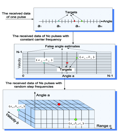
Figure 1: Illustration of the decoupled angle-velocity-range estimation approach

Solving an $\ell_{1}$ minimization problem requires polynomial time in the dimension of $\mathbf{s}$. Let us discretize the angle, Doppler and range space into $[a_{1},\ldots,a_{N_{a}}]$, $[b_{1},\ldots,b_{N_{b}}]$ and $[c_{1},\ldots,c_{N_{c}}]$, respectively. The joint estimation of angle, velocity and range requires complexity of $\mathcal{O}((N_{a}N_{b}N_{c})^{3})$. For large $N_{a}$, $N_{b}$ and $N_{c}$, the complexity cost of the CS approach would be prohibitive. In this section, we propose a decoupled angle-velocity-range estimation approach to lower the complexity burden. Let us consider the case of slowly moving targets, i.e., $f_{k}T_{s}L\ll 1$. In this case, the Doppler shift within a pulse can be ignored. We propose to first transmit $N_{c}$ pulses with constant carrier frequency, and then transmit $N_{s}$ pluses with random step frequency. Based on these pulses, the estimation proceeds in the following steps.

Step 1: For the data collected during one pulse, the phase terms associated with range and Doppler are constant over all receive nodes. Therefore, we can estimate the azimuth angle by discretization of the angle space only, as illustrated in the top graph of Fig. 1 and described in [13] in detail. The same process can be repeated on a number of different received pulses. Let $\Gamma_{i}$ denote the set of angle estimates obtained based on the $i$-th pulse. The union of the angle-estimate sets $\Gamma_{1},\ldots,\Gamma_{N_{p}}$ are the angle estimates that are provided to the next step.

Step 2: As described in Section III, the range information can be excluded from the basis matrix for the data with constant carrier frequency. Therefore, we can extract the Doppler information by applying CS to the data collected during the first $N_{c}$ pulses. The corresponding basis matrix can be formed based on the above obtained initial angle estimates and a discretization of the Doppler space as shown in the middle graph of Fig. 1.

Step 3: By processing the received signal of $N_{s}$ pulses with the random stepped frequencies, we can extract range information as described in Section III with the important difference that only the range axis needs to be discretized and used along with the angle-velocity estimates produced in Step 2 (see the bottom graph of Fig. 1).

The complexity of Step 1, Step 2 and Step 3 are respectively $\mathcal{O}(A(N_{a})^{3})$, $\mathcal{O}((BN_{b})^{3})$ and $\mathcal{O}((CN_{c})^{3})$, where $A$, $B$ and $C$ are scalars much smaller than $N_{a}$, $N_{b}$ and $N_{c}$. Therefore, the total complexity of the decoupled scheme is $\mathcal{O}(A(N_{a})^{3}+(BN_{b})^{3}+(CN_{c})^{3})$. For large $N_{a}$, $N_{b}$ and $N_{c}$, it holds that $\mathcal{O}(A(N_{a})^{3}+(BN_{b})^{3}+(CN_{c})^{3})\ll\mathcal{O}((N_{a}N_{b}N_{c})^{3})$ which implies significant savings.

V Simulations

We consider a MIMO radar system with the transmit/receive nodes uniformly distributed on a disk of radius $10$m. The center carrier frequency is $f=5GHz$ and the pulse repetition interval is $T=\frac{1}{4000}s$. Each transmit node uses orthogonal QPSK waveforms. The received signal is corrupted by zero mean Gaussian noise. The SNR is set to $0$ dB. The SNR here is defined as the ratio of power of transmit waveform to that of thermal noise at a receive node. A jammer is located at angle $7\textordmasculine$ and transmits an unknown Gaussian random waveform with amplitude 60. The target reflection coefficients are all one.

Fig. 2 compares the performance of velocity estimation with constant carrier frequency and randomly stepped frequency. The target scenes shown in Fig. 2 are generated via $100$ independent and random runs. The grey scale represents the times a target detected by CS occupies a particular grid point in the target scene. A lighter color indicates a higher occurrence frequency of a target. To highlight the velocity estimation, we consider an extreme case in which three targets are moving in the same direction of $0\textordmasculine$ and have the same range at the initial time, i.e. $R=1500m$. The radial velocities of the three targets are $170m/s$, $175m/s$ and $180m/s$, respectively. The unambiguous velocity for the constant carrier frequency $f=5GHz$ is $120m/s$. The possible ambiguous estimates of three targets are $50m/s$, $55m/s$ and $60m/s$, respectively. The number of transmit nodes and receive nodes are $M_{t}=30$ and $N_{r}=5$, respectively. $M=30$ measurements are obtained at each receive node. The top graph shows the true target scene. We consider the worst case for velocity estimation in which the three targets are located at adjacent grid points in the velocity domain. Therefore, a single bright spot appears in the target scene instead of three spots. The last three graphs demonstrate the target scenes produced by the CS approach with constant and step carrier frequency. It can be seen from Fig. 2 that the introduction of random step frequency can eliminate the velocity ambiguity by using sufficiently many pulses ($N_{p}=10$). In sharp contrast, the use of constant carrier frequency always yields the ambiguous estimates around $50m/s$ using the same number of pulses.

Fig. 3 shows the estimates of target locations in the angle-velocity-range space using the proposed decoupled method. Three targets are moving in the directions of $\{-0.5\textordmasculine,0\textordmasculine,0.5\textordmasculine\}$. The radial velocity of the three targets are $70m/s$, $75m/s$ and $80m/s$, respectively. The corresponding ranges are $1200m/s$, $1250m/s$ and $1200m/s$. We sample the angle-velocity-range space by the increment $(0.5\textordmasculine,5m/s,50m)$. The number of transmit nodes and receive nodes are $M_{t}=30$ and $N_{r}=30$, respectively. $M=30$ measurements are obtained at each receive node. The transmitters first send $N_{c}=5$ pulses with constant carrier frequency and then $N_{s}=5$ pulses with randomly stepped frequency. The top and bottom graphs show respectively the true target locations and the estimates produced by the decoupled angle-Doppler-range scheme in 100 random and independent runs. We can see that the information on the three targets is exactly recovered in each of the $100$ runs. A false target arises in only one out of 100 runs. The false target is quite close to the first target, i.e., $(-0.5\textordmasculine,80m/s,1100m)$. The decoupled scheme requires only $0.002\%$ of the complexity of joint estimation of angle, velocity and range.

VI Conclusion

We have proposed a CS based MIMO radar approach for obtaining angle-velocity-range estimates. First, we have introduced a step frequency approach in each transmit node, which not only achieves high range resolution but also improve the unambiguous velocity. Further, a decoupled angle-velocity-range estimation scheme has been proposed to alleviate the complexity burden of CS applied to the joint angle-velocity-range estimation. The proposed scheme can dramatically reduce the computational cost of CS and still achieve good performance.

Acknowledgment

The authors wish to thank Dr. Rabinder Madan for essential contributions to this work.

Appendix A Appendix A

For a given pair $(k,k^{\prime}),k\neq k^{\prime}$, satisfying $a_{k}=a_{k^{\prime}}$ and $b_{k^{\prime}}-b_{k}=\Delta b$, $h({\bf\Delta}f)$ is proportional to the ratio of $p_{kk^{\prime}}$ to $p_{kk}$, which reveals the effect of $\mathbf{\Delta}f$ on the correlation of columns corresponding to the adjacent grid points in the velocity dimension. Instead of analyzing $h(\mathbf{\Delta}f)$, we define another function for convenience as follows:

$$C(\mathbf{\Delta}f)=h^{2}(\mathbf{\Delta}f)=\sum_{m=1}^{N_{p}}\sum_{n=1}^{N_{p}}e^{j\alpha((m-n)+\Delta f_{m}(m-1)-\Delta f_{n}(n-1))}$$

$$=N_{p}+\sum_{m=1}^{N_{p}}\sum_{n=m+1}^{N_{p}}2\cos(\alpha((m-n)+\Delta f_{m}(m-1)$$

$$-\Delta f_{n}(n-1)))$$ (16)

$C(\mathbf{\Delta}f)$ can be expanded by the Taylor series of the first order as

$$C(\mathbf{\Delta}f)\approx C(\mathbf{0})+\sum_{m=1}^{N_{p}}\Delta f_{m}\frac{\partial C(\mathbf{\Delta}f)}{\partial\Delta f_{m}}|_{{\bf\Delta}f={\bf 0}}$$

$$=C(\mathbf{0})-2\alpha\sum_{m=\lfloor N_{p}/2\rfloor+1}^{N_{p}}\sum_{n=m-1}^{N_{P}+1-m}(\Delta f_{m}(m-1)$$

$$-\Delta f_{N_{p}+1-m}(N_{p}-m))\sin(\alpha n)$$ (17)

$\sum_{m=1}^{N_{p}}\Delta f_{m}\frac{\partial C(\mathbf{\Delta}f)}{\partial\Delta f_{m}}|_{{\bf\Delta}f={\bf 0}}$ is required to be negative for $C(\mathbf{\Delta}f)<C(\mathbf{0}),\mathbf{\Delta}f\neq 0$. Therefore, sufficient conditions that guarantees $C(\mathbf{\Delta}f)<C(\mathbf{0}),\mathbf{\Delta}f\neq 0$ are

• $\frac{\Delta f_{m}}{\Delta f_{N_{p}+1-m}}\geq\frac{N_{p}-m}{m-1}$, $m>\lfloor N_{p}/2\rfloor$

  ($\Delta f_{m}=m\Delta f$ satisfies this condition);

• $\sin(\alpha n)>0$ for $n=1,\ldots,N_{p}-1$.

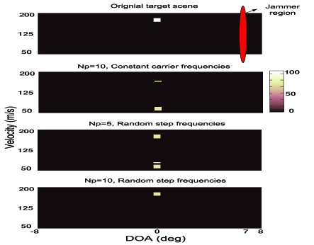
Figure 2: Velocity estimates using constant carrier frequency and randomly stepped frequency for $M=M_{t}=30$ and $N_{r}=5$.

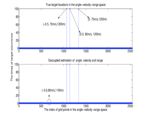
Figure 3: Target scenes produced by decoupled angle-velocity-range estimation with randomly stepped frequency for $M=M_{t}=N_{r}=30$ and $N_{c}=N_{s}=5$.

References

- [1] E. Fishler, A.M. Haimovich, R. Blum, D. Chizhik, L. Cimini and R. Valenzuela, “MIMO radar: An idea whose time has come,” in Proc. IEEE Radar Conf., Philadelphia, PA, pp. 71-78, Apr. 2004.
- [2] A.M. Haimovich, R.S. Blum and L.J. Cimini, “MIMO radar with widely separated antennas,” IEEE Signal Processing Magazine, vol. 25, issue 1, pp. 116 - 129, 2008.
- [3] P. Stoica and J. Li, “MIMO radar with colocated antennas,” IEEE Signal Processing Magazine, vol. 24, pp. 106 - 114, issue 5, 2007.
- [4] D.V. Donoho, “Compressed sensing,” IEEE Trans. Information Theory, vol. 52, pp. 1289-1306, no. 4, April 2006.
- [5] E.J. Candes and M.B. Wakin, “An introduction to compressive sampling [A sensing/sampling paradigm that goes against the common knowledge in data acquisition],” IEEE Signal Processing Magazine, vol. 25, pp. 21 - 30 , March 2008.
- [6] R. Baraniuk and P. Steeghs, “Compressive radar imaging,” Proc. Radar Conference, pp. 128 - 133, April, 2007.
- [7] A.C. Gurbuz, J.H. McClellan and W.R. Scott, “Compressive sensing for GPR imaging,” Proc. 41th Asilomar Conf. Signals, Syst. Comput, pp. 2223-2227, Pacific Grove, CA, Nov. 2007.
- [8] M. Herman and T. Strohmer, “Compressed rensing radar,” in Proc. IEEE Int’l Conf. Acoust. Speech Signal Process, Las Vegas, NV, pp. 2617 - 2620, Mar. - Apr. 2008.
- [9] A.P. Petropulu, Y. Yu and H.V. Poor, “Distributed MIMO radar using compressive sampling,” Proc. 42nd Asilomar Conf. Signals, Syst. Comput, Pacific Grove, CA, Nov. 2008.
- [10] C. Chen and P.P. Vaidyanathan, “MIMO radar space-time adaptive processing using prolate spheroidal wave functions,” IEEE Trans. Signal Process., vol. 56, no. 2, pp. 623 - 635, Feb. 2008.
- [11] Y. Yu, A.P. Petropulu and H.V. Poor, “MIMO radar using compressive sampling,” IEEE Journal of Selected Topics in Signal Processing, to appear in December 2009.
- [12] G.S. Gill, “High-Resolution Step Frequency Radar” Ultra-Wideband Radar Technology, CRC Press.
- [13] Y. Yu, A.P. Petropulu and H.V. Poor, “MIMO radar based on reduced complexity compressive sampling,” IEEE Radio and Wireless Symposium 2010, New Orleans, LA, Jan. 2010.
- [14] E.J. Candes and T. Tao, “The Dantzig selector: Statistical estimation when is much larger than ,” Ann. Statist., vol. 35, pp. 2313-2351, 2007.
- [15] E.J. Candes and J. Romberg, “-MAGIC: Recovery of sparse signals via convex programing,” http://www.acm.caltech.edu/l1magic/, October 2008.
- [16] J.A. Tropp and A.C. Gilbert, “Signal recovery from random measurements via orthogonal matching pursuit,” IEEE Trans. Info. Theory, pp. 4655-4666, 2007.
- [17] E.J. Candes, J.K. Romberg and T. Tao, “Stable signal recovery from incomplete and inaccurate measurements,” Communications on Pure and Applied Mathematics, vol. 59, pp. 1207-1223, 2006.