Inverse problem: Reconstruction of modified gravity action in Palatini formalism by Supernova Type Ia data

Abstract

We introduce in $f(R)$ gravity–Palatini formalism the method of inverse problem to extract the action from the expansion history of the universe. First, we use an ansatz for the scale factor and apply the inverse method to derive an appropriate action for the gravity. In the second step we use the Supernova Type Ia data set from the Union sample and obtain a smoothed function for the Hubble parameter up to the redshift 1.7. We apply the smoothed Hubble parameter in the inverse approach and reconstruct the corresponding action in $f(R)$ gravity. In the next step we investigate the viability of reconstruction method, doing a Monte-Carlo simulation we generate synthetic SNIa data with the quality of union sample and show that roughly more than 1500 SNIa data is essential to reconstruct correct action. Finally with the enough SNIa data, we propose two diagnosis in order to distinguish between the $\Lambda$CDM model and an alternative theory for the acceleration of the universe.

PACS numbers: 04.50.+h, 95.36.+x, 98.80.-k

]

I Introduction

Combination of SNIa+CMB data shows that universe is in the positive acceleration phase [1, 2]. This result is in contradiction with our expectation from the behavior of the ordinary matter. The simplest solution is assuming a cosmological constant in the Einstein field equation as a constant of integration [3]. While this simple modification explains the observational data[4], however the cosmological constant suffers from the fine tuning and coincidence problems[5]. One of the solutions is introducing a scalar field which provides a time dependent negative equation of state [6].

The other possibility is the modification of the gravity law in such a way that it behaves as standard General Relativity in strong gravitational regimes and repulse particles in the low density cosmological scales [7]. The modified gravity models can be examined with three category of observations of (a) cosmological dynamics [8], (b) local gravity [9] and (c) the evolution of large scale structure [10].

In this work we use SNIa data to reconstruct an appropriate $f(R)$ gravity model in Palatini formalism [11] with the inverse method. The method is the extension of the work introduced for the metric formalism by Rahvar and Sobouti in [12]. The inverse method also is introduced in the work by Capozziello et al.[13] in the metric formalism. In this method we need to know the dynamics of Hubble parameter from the observational data. Many methods for the extraction of the Hubble parameter have been introduced in the literature [14]. Here we use the smoothing method suggested by Shafieloo et al.[15] and apply it to the SNIa Union sample [16]. We use $H(z)$ in the inverse method algorithm to reconstruct the corresponding action. We test the reliability of this method by doing a Monte-Carlo simulation and generating the synthetic SNIa data according to an action and comparing the reconstructed action with the original one. Finally we introduces two diagnosis for distinguishing standard $\Lambda$CMD model from the alternative models.

The structure of this article is as follows: In section II we introduce $f(R)$ modified gravity in Palatini formalism, derive the equation of motion and obtain the dependence of Hubble parameter to the Ricci scalar and scale factor. In section III we introduce the method of inverse problem in Palatini $f(R)$ gravity. In section IV we use the method to the real data of SNIa, smoothing the supernova data we extract the Hubble parameter in terms of redshift and apply it to extract the action [15]. Also in order to show the level of confidence of our results, we simulate 100 realization of SNIa data to extract the Hubble parameter and compare it with that obtained directly from fitting to the model. In the section V, we examine the viability of reconstruction method and dependence of the results to the number of SNIa data. In section VI we propose two diagnosis as probe to distinguish between the $\Lambda$CDM and the alternative models. Section VII concludes the paper.

II modified gravity in Palatini formalism

For $f(R)$ gravity, there are two main approaches to obtain the field equation. The first one is so-called metric formalism which is obtained by the variation of the action with respect to the metric. In this case the derived field equation is a fourth order nonlinear differential equation. In the second approach, which is called Palatini formalism, the connection and metric are considered as independent fields and the variation of action with respect to these fields results in a set of second order differential equations. The Palatini formalism is a plausible candidate to be the effective classical theory of gravity from a more fundamental theory of Loop Quantum Gravity [17].

Let us take a general form of the action in Palatini formalism as:

$$S[f;g,\hat{\Gamma},\Psi_{m}]=-\frac{1}{2\kappa}\int{d^{4}x\sqrt{-g}f(R)+S_{m}[g_{\mu\nu},\Psi_{m}]},$$ (1)

where $\kappa=8\pi{G}$ and $S_{m}[g_{\mu\nu},\Psi_{m}]$ is the action of matter depends on the metric $g_{\mu\nu}$ and the matter field $\Psi_{m}$. $R=R(g,\hat{\Gamma})=g^{\mu\nu}{R_{\mu\nu}}(\hat{\Gamma})$ is the generalized Ricci scalar and $R_{\mu\nu}$ is the Ricci tensor made of affine connection. Varying action with respect to the metric results in:

$$f^{\prime}(R)R_{\mu\nu}(\hat{\Gamma})-\frac{1}{2}f(R)g_{\mu\nu}=\kappa T_{\mu\nu},$$ (2)

where prime is the derivative with respect to the Ricci scalar and $T_{\mu\nu}$ is the energy momentum tensor

$$T_{\mu\nu}=\frac{-2}{\sqrt{-g}}\frac{\delta S_{m}}{\delta g^{\mu\nu}}.$$ (3)

On the other hand varying the action with respect to the connection results in:

$$\hat{\nabla_{\alpha}}[f^{\prime}(R)\sqrt{-g}g^{\mu\nu}]=0,$$ (4)

where $\hat{\nabla}$ is the covariant derivative defined from parallel transformation and is given by the affine connection. From equation (4), we define a new metric, $h_{\mu\nu}=f^{\prime}(R)g_{\mu\nu}$ conformally related to the physical metric where the connection is the Christoffel symbol of this new metric.

We apply flat FRW metric (namely $K=0$) for the universe

$$ds^{2}=-dt^{2}+a(t)^{2}\delta_{ij}dx^{i}dx^{j},$$ (5)

and assume that universe is filled with a perfect fluid with the energy-momentum tensor of $T^{\nu}_{\mu}=diag(-\rho,p,p,p)$. Using the metric and energy momentum tensor in Eq.(2), we obtain the generalized FRW equations. It should be noted that the conservation law of energy-momentum tensor, $T^{\mu\nu}{}_{;\mu}=0$ is satisfied according to the covariant derivative with respect to the metric and this definition guarantees the motion of particles on geodesic [18]. Combination of $G_{00}$ and $G^{i}_{i}$ results in[19]:

$$(H+\frac{1}{2}\frac{\dot{f^{\prime}}}{f^{\prime}})^{2}=\frac{1}{6}\frac{\kappa(\rho+3p)}{f^{\prime}}+\frac{1}{6}\frac{f}{f^{\prime}}.$$ (6)

Taking the trace of equation (2) results in

$$Rf^{\prime}(R)-2f(R)=\kappa T,$$ (7)

where $T=g^{\mu\nu}T_{\mu\nu}=-\rho+3p$. The time derivative of this equation results $\dot{R}$ in terms of time derivative of density and pressure. Using the equation of state of cosmic fluid $p=p(\rho)$ and the continuity equation, the time derivative of Ricci obtain as:

$$\dot{R}=3\kappa H\frac{(1-3dp/d\rho)(\rho+p)}{Rf^{\prime\prime}-f^{\prime}(R)}.$$ (8)

To obtain generalized first FRW equation we start with equation (7) and obtain the density of matter in terms of Ricci scalar as:

$$\kappa\rho=\frac{2f-Rf^{\prime}}{1-3\omega},$$ (9)

where $w=p/\rho$. We substitute equation (9) in (6) and use equation (8) to change the time derivative to ${d}/{dR}$. We rewrite equation (6) as follows:

$$H^{2}=\frac{1}{6(1-3\omega)f^{\prime}}\frac{3(1+\omega)f-(1+3\omega)Rf^{\prime}}{\left[1+\frac{3}{2}(1+\omega)\frac{f^{\prime\prime}(2f-Rf^{\prime})}{f^{\prime}(Rf^{\prime\prime}-f^{\prime})}\right]^{2}}.$$ (10)

On the other hand using equation (7) and continuity equation, the scale factor can be obtained in terms of Ricci scalar

$$a=\left[\frac{1}{\kappa\rho_{0}(1-3\omega)}(2f-Rf^{\prime})\right]^{-\frac{1}{3(1+\omega)}},$$ (11)

where $\rho_{0}$ is the energy density and $a_{0}$ is the scale factor (set to one, i.e.$~{}a_{0}=1$) at the present time. Now for a generic modified action, omitting Ricci scalar in favor of the scale factor between equations (10) and (11) we can obtain the dynamics of universe (i.e. $H=H(a)$).

For the simple case of matter dominant epoch $\omega=0$ which is in our concern, these equations reduce to:

$$H^{2}=\frac{1}{6f^{\prime}}\frac{3f-Rf^{\prime}}{\left[1+\frac{3}{2}\frac{f^{\prime\prime}(2f-Rf^{\prime})}{f^{\prime}(Rf^{\prime\prime}-f{{}^{\prime}})}\right]^{2}}$$ (12)

$$a=\left[\frac{1}{\kappa\rho_{0}}(2f-Rf^{\prime})\right]^{-\frac{1}{3}}$$ (13)

III Inverse Method in Palatini formalism

In this section we introduce the inverse method to extract $f(R)$ action in Palatini formalism from the dynamics of the universe. This method has been studied in the work by Rahvar and Sobuti in the metric formalism [12] and we extend it to the Palatini formalism.

Replacing $f$ with the first derivatives of action from the equation (7),

$$f(R)=\frac{1}{2}[{RF}-\kappa(3p-\rho)],$$ (14)

equation (6) can be written as follows:

$$(H+\frac{1}{2}\frac{\dot{F}}{F})^{2}=\frac{R}{12}+\frac{\kappa}{4F}(\rho+p).$$ (15)

where $F$ is defined as $F={df}/{dR}$. It should be noted that Ricci tensor in the Palatini formalism is given in terms of the conformal metric of $h_{\mu\nu}=F(R)g_{\mu\nu}$. Substituting the new metric in the definition of Ricci scalar results in:

$$R_{\mu\nu}=R_{\mu\nu}(g)+\frac{3}{2}\frac{\nabla_{\mu}F\nabla_{\nu}F}{F^{2}}-\frac{\nabla_{\mu}\nabla_{\nu}F}{F}-\frac{1}{2}g_{\mu\nu}\frac{\nabla_{\alpha}\nabla^{\alpha}F}{F},$$ (16)

where $R_{\mu\nu}(g)$ is the Ricci tensor defined in terms of metric $g_{\mu\nu}$. By taking trace from equation (16) we obtain relation between the Ricci scalar in Palatini and metric as:

$$R=R(g)+\frac{3}{2}\frac{\nabla_{\alpha}F\nabla^{\alpha}F}{F^{2}}-\frac{3\nabla_{\alpha}\nabla^{\alpha}F}{F}.$$ (17)

On the other hand using the FRW metric, $R(g)$ as the Ricci scalar in metric formalism is given by the Hubble parameter as:

$$R(g)=6\dot{H}+12H^{2},$$ (18)

where for simplicity in the calculation we rewrite this equation by changing the time derivative to the redshift derivative. In what follows we use prime for the derivative with respect to the redshift.

$$R(g)=-6HH^{\prime}(1+z)+12H^{2}.$$ (19)

For the Ricci scalar in Palatini formalism from equation (17), we obtain:

$$R=-6HH^{\prime}(1+z)+12H^{2}-\frac{3}{2}H^{2}(1+z)^{2}(\frac{F^{\prime}}{F})^{2}$$ (20)

$$+ 3(1+z)^{2}HH^{\prime}\frac{F^{\prime}}{F}-6H^{2}(1+z)\frac{F^{\prime}}{F}+3H^{2}(1+z)^{2}\frac{F^{\prime\prime}}{F}$$ (21)

Substituting this equation in (15) results in a differential equation for the evolution of $F$ as a function of redshift:

$$F^{\prime\prime} - \frac{3}{2}\frac{F^{\prime 2}}{F}+F^{\prime}(\frac{H^{\prime}}{H}+\frac{2}{1+z})$$ (22)

$$- \frac{2H^{\prime}}{H(1+z)}F+\frac{\kappa}{H^{2}(1+z)^{2}}(\rho+p)=0.$$ (23)

In the matter dominant epoch we rewrite this equation by putting $p=0$ and $\rho=\rho_{0}(1+z)^{3}$, where we can replace $\kappa\rho_{0}$ with $3H_{0}^{2}\Omega_{m}$. It should be noted that the definition of the $\Omega_{m}$ is different from that in the standard FRW equations.

For a given dynamics of universe (i.e. $a(t)$), we can extract the Hubble parameter in terms of redshift, applying it in equation (23) will provide $F$ in terms of redshift. On the other side we can calculate the Ricci scalar from equation (20) in terms of redshift. Eliminate $z$ in favor of Ricci scalar results in $F(R)$. Finally by the numerical integration of this function we can obtain the modified gravity action, $f(R)$.

In the rest of this section to test this algorithm we use an ansatz for the scale factor and try to extract the corresponding action from a given dynamics. We apply the following ansatz for the scale factor proposed in [12]:

$$a(\tau)=\frac{1}{1+p}(\tau)^{\frac{2}{3}}[1+p\tau^{\frac{2\alpha}{3}}]$$ (24)

in which $\tau=tH_{0}$ is a dimensionless time parameter defined in the interval of 0 to 1 and $H_{0}$ is the Hubble parameter at the present time. This proposed dynamics has two free parameters of $\alpha$ and $p$. We obtain the corresponding Hubble parameter from this scale factor and consequently the distance modulus and compare the model with the observed SNIa data. The best value for the parameters of model has been obtained roughly, $p=\frac{1}{3}$ and $\alpha=2$ in [12]. Substituting the scale factor in equation (23), we obtain the deviation parameter of $\xi\equiv F-1$ from GR as a function of redshift, which is plotted in Figure (1).

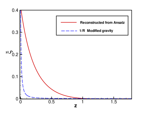
FIG. 1.: Deviation parameter $\xi=F(R)-1$ is obtained from the ansatz scale factor (solid-line) is compared with $\xi$-parameter of $1/R$ modified gravity (dashed-line) in terms of redshift. For the redshifts $z>1$, the $f(R)$ gravity model converge to the Einstein-Hilbert action.

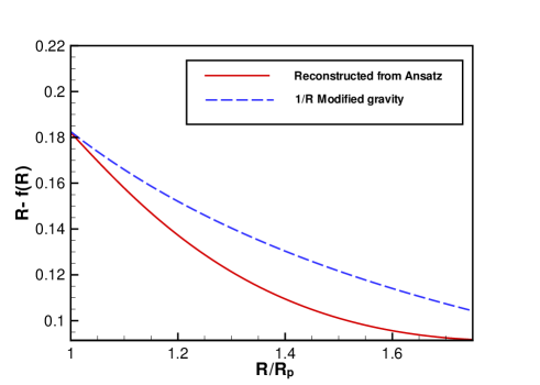
FIG. 2.: The difference of modified gravity action from the Einstein-Hilbert action is plotted versus Ricci scalar (solid-line) and compared with the action of $f(R)=R-\frac{\mu^{4}}{R}$ (dashed-line). The Ricci scalar is normalized to its value at the present time, $R_{p}$.

In order to reconstruct the action in terms of Ricci action, we obtain the Ricci scalar in terms of redshift and finally by eliminating redshift between $F$ and Ricci scalar, we obtain $F=F(R)$. Integrating this function provides action in terms of Ricci scalar. We also plot the $\xi$-parameter of $1/R$ modified gravity for comparison with the reconstructed modified gravity in Figure (1) and $R-f(R)$ as a function of $R$ in Figure (2). Comparison of the extra term with the Einstein-Hilbert action roughly resembles to $\mu^{4}/R$ function with $\mu^{2}\sim 10^{-1}R_{p}$ where $R_{p}$ is the present value of Ricci scalar.

IV Reconstruction of the dynamic of the Universe by SNIa data

In section III, we showed that it is possible to reconstruct the modified gravity action by knowing the dynamics of the universe. In this section, we use SNIa cosmological data to obtain the Hubble parameter and consequently reconstruct the action of modified gravity.

The dynamics of Hubble parameter, $H(z)$, can be obtained if the distance modulus of Supernovas data as a function of redshift is known. In FRW–flat universe, the Hubble parameter is related to the distance modulus of SNIa as follows:

$$H(z)=[\frac{d}{dz}(\frac{d_{L}(z)}{1+z})]^{-1}.$$ (25)

The main challenging point in this procedure is the limited number of observed SNIa which impose an uncertainty in calculating the continues function for $H(z)$. The overall number of Supernovas which has been detected is in the order of 300-400. We use the latest Supernova data of the Union sample to extract the Hubble parameter [16]. To make a continues Hubble parameter, we follow the procedure known as reconstruction method, proposed by Shafieloo et al. in [15]. In this algorithm, a non-parametric function is used for smoothing the distance modulus of supernova data over the redshift. Here we choose a guess model resemble to the observed distance modulus of the supernova data. In the next step we subtract the distance modulus of the observed data from the guess model using a gaussian function for smoothing the observed data as follows:

$$\mu^{d}(z)=N(z)\sum_{i}[\mu^{g}(z)-\mu^{obs}(z_{i})]\exp{\frac{-(z-z_{i})^{2}}{2\Delta^{2}}},$$ (26)

where

$$N(z)^{-1}=\sum_{i}\exp[\frac{-(z-z_{i})^{2}}{2\Delta^{2}}],$$ (27)

where $z_{i}$ represents the redshift of each SNIa in the Union sample. The sum term is considered for all 307 Union sample data, $\mu^{obs}(z_{i})$ is the observed distance modulus and $\mu^{g}(z)$ is a continues guess model for the distance modulus. $N(z)$ is a normalization factor and $\Delta$ is a suitable redshift window function. $\mu^{d}(z)$ is a smoothed continues function for the residual of luminosity distance in terms of redshift. Now the corrected distance modulus is added to the guess model to generate the new smooth function for the distance modulus:

$$\mu^{s}(z)=\mu^{g}(z)+\mu^{d}(z).$$ (28)

We repeat this procedure using $\mu^{s}(z)$ as the new guess function. It can be shown that after a finite time of this irritation, $\chi^{2}$ of the smoothed function with respect to observed data will converge to a fixed value. It means that we will find a continues distance modulus function with the best fit to the real data. It is shown in [15] that the result of the best continues function is independent of the choice of the first guess model. Having the the smoothed luminosity distance we use equation (25) to obtain the Hubble parameter H(z). Another point is that the results will clearly depend upon the value of $\Delta$ in equation (26). A large value of $\Delta$ produce a smooth result, but the accuracy of reconstruction worsens, while small value $\Delta$ gives more accurate, but noisy result. Considering the frequency of SNIa data observed in the Union sample, we choose $\Delta=\sqrt{M}(1+z)\Delta_{0}$ for the window function, where M is the number of irritation need to converge $\chi^{2}$ and $\Delta_{0}=N^{-1/3}$ where N is the number of SNIa [15].

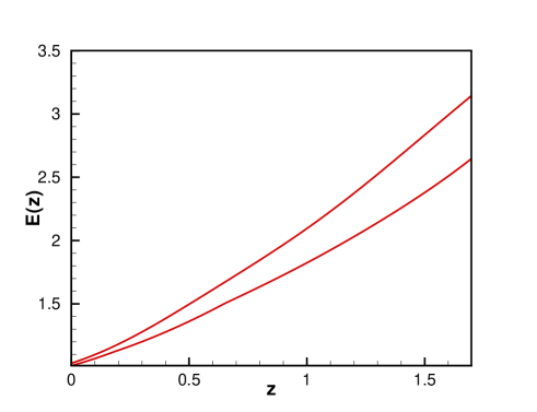
FIG. 3.: The uncertainty in $E(z)=\frac{H}{H_{0}}$ from the smoothing method, resulting from the Monte-Carlo simulation. We generate one hundred realization for the distance modulus and obtain the Hubble parameter which all these continues functions reside inside the boundaries in the figure.

In what follows we find the uncertainty in $H(z)$ from this method to use it for reconstructing the appropriate action in the Palatini formalism. For this purpose we do a Monte-Carlo simulation, generating 100 realization of SNIa data and using the same distribution of SNIa in terms of redshift reported by Kowalski et al.[16]. Also we use the same error bars of distance modulus in the observed data. In order to simulate the synthetic distance modulus of SNIa, we assume a dark energy model for the universe with a constant equation of state of $\omega=-0.75$. Choosing $\Lambda$CDM as the guess model for these data, we obtain the Hubble parameter $E(z)=H(z)/H_{0}$ for $100$ realization of supernova data. Figure (3) shows the boundaries for $E(z)$, resulted from 100 realization of Supernova data.

Now we can apply this uncertainty to $H(z)$, resulting from the smoothing procedure on the real Union sample [20]. We plot the Hubble parameter from the Union sample as shown in Figure (4) with a margin represents the uncertainty that is obtained form the Monte-Carlo simulation. Using the method described in section III, we extract the corresponding modified gravity in Palatini formalism. The parameter of $\xi={df(R)}/{dR}-1$ in terms of Ricci scaler shows a small deviation from the Einstein-Hilbert action as shown in Figure (5) with the uncertainty of this parameter. Here the deviation from the Einstein-Hilbert action is in the order of $\xi\sim 10^{-3}$. We ask the reliability of this result in terms of the number of SNIa data. In the next section we will discus about this issue.

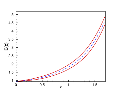
FIG. 4.: Dashed line is the reconstructed Hubble parameter from SNIa Union sample data. Bold lines are the confidence level of Hubble parameter.

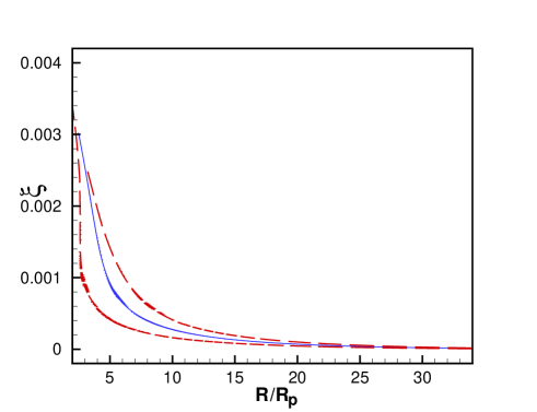
FIG. 5.: The bold line shows the reconstructed modified gravity $\xi\equiv F-1$ parameter versus Ricci scalar normalized to its present value. The dashed lines show the confidence level of the $\xi$ parameter corresponds to the uncertainty of the Hubble parameter resulting from the smoothing procedure.

V Viability of smoothing method and the number of SNIa data

In this section we examine the viability of smoothing of the Hubble parameter. The results will be applied to the modified gravity models in the next section.

According to the methodology of the smoothing procedure, the Hubble parameter depends on the quantity and quality of SNIa data. Similar to the simulation in the previous section we generate 100 realization of 307 SNIa data, using the redshift and the uncertainty of the distance modulus in the Union sample within the framework of $\Lambda$CDM model. We generate continues Hubble parameter with the margin of uncertainty which is shown in Figure (6). On the other hand we obtain the Hubble parameter in $\Lambda$CDM model though fitting the observed distance modulus of the data to the model as shown in Figure (6). The margin represents 1$\sigma$ level of confidence for the Hubble parameter. Comparing the uncertainties from these two methods show that the smoothing method is not reliable with 307 number of supernova data.

We increase the number of SNIa data with the quality of Union sample to have the same uncertainty in the Hubble parameter from the two methods. For $N>1500$ as shown in Figure (6) we can rely on the smoothing method. We can repeat this simulation with precise data than the Union sample to achieve this goal with a smaller number of Supernova data.

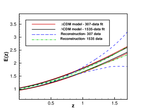
FIG. 6.: Dashed lines and dotted dashed line are the reconstructed Hubble parameters from 307 and 1535 SNIa data, respectively. Solid lines are 1-$\sigma$ confidence level of Hubble parameter from data fitting to 307 and 1535 data in $\Lambda$CDM model.

VI Distinguishing between the Modified Gravity models and $\Lambda$CDM

In this section we present two diagnosis in order to distinguish between $\Lambda$CDM from an alternative model. The first method is (a) Comparison of the Hubble parameters and the second method is (b) the $\Xi$-function. Both of diagnosis are applicable by using the inverse method.

A Comparison of the Hubble parameters

In the previous section we have seen the smoothing method to generate a continues Hubble parameter from the observed data. If the dynamics of universe follows rather than the $\Lambda$CDM model, can we distinguish the real model of the universe, knowing the Hubble parameter from the data ?

We can compare the reconstructed Hubble parameter directly from the observed data with that of obtained from fitting data to the $\Lambda$CDM model. We subtract the two Hubble parameters and compare it with $1\sigma$ deviation of the smoothed Hubble parameter. As we simulated in the previous section using $N>1500$ is sufficient to reliable on the uncertainty of the Hubble parameter.

We use $f(R)=R-\frac{\mu^{4}}{R}$ action in Palatini formalism and generate $1535$ supernova data with the quality of the Union sample. Using the smoothing method we obtain the Hubble parameter. On the other hand we fit the generated data with the $\Lambda$CDM model. Figure (7) compares the two Hubble parameters and shows that for the redshifts with $z>1$, the two models are distinguishable.

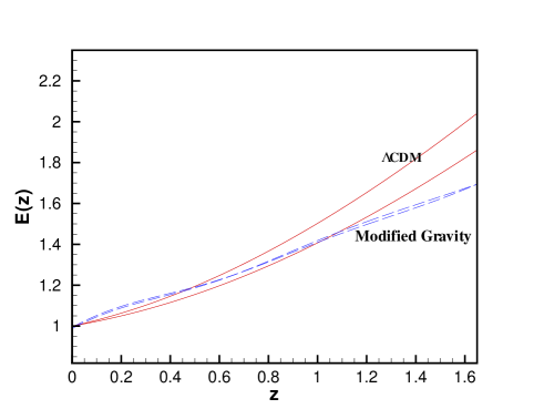
FIG. 7.: The solid-line is the Hubble parameter with 1-$\sigma$ error bar from fitting the simulated data to the $\Lambda$CDM model. The dashed-line is the confidence level of Hubble parameter extracted from the smoothing method of the Hubble parameter. The figure shows the deviation of the two curve for $z>1$.

B The method of $\Xi$-function

We define a new criterion to distinguish the $\Lambda$CDM from an alternative model as follows:

$$\Xi\equiv\frac{2E(z)E^{{}^{\prime}}(z)}{3(1+z)^{2}},$$ (29)

where prime is differential with respect to the redshift. For the case of $F=1$ in $\Lambda$CDM universe, from equation (23), $\Xi$ reduces to $\Xi=\Omega_{m}^{0}$. If we have the smoothed normalized Hubble parameter from the observed data, $E(z)$, then $\Xi$ can be obtained. Any deviation from a constant value for this function is a diagnosis for the $\Lambda$CDM universe. This method is applicable both for the dark energy and modified gravity models. Let us take $\omega(z)$ as the equation of state of dark energy, we can use FRW equations to obtain $\Xi$ as follows:

$$\Xi=\Omega_{m}^{0}+(1-\Omega_{m}^{0})\frac{1+\omega(z)}{(1+z)^{3}},$$ (30)

where for the constant value of the equation of state, $\omega(z)=-1$, this equation reduces to $\Xi=\Omega_{m}^{0}$.

In order to show the deviation from the Einstein-Hilbert action, we can calculate $\Xi-\Omega_{m}^{(0)}$ as a function of redshift. Here we know $\Omega_{m}^{(0)}$ from a direct cosmological observations such as gravitational weak lensing.

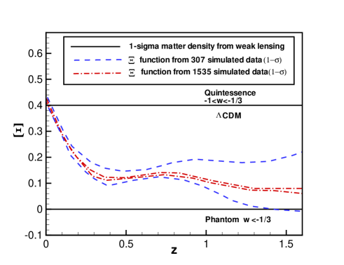
FIG. 8.: $\Xi$-function versus redshift is plotted for two series of SNIa data, with 1$\sigma$ level of confidence. The dash-lines and dashed-dotted lines indicate for 307 and 1535 data respectively. Solid lines indicate the matter density of universe derived from gravitational weak lensing.

To show how this method works we generate SNIa data from $f(R)=R-\mu^{4}/R$ action resemble to the Union sample and after smoothing the Hubble parameter, we plot $\Xi$ as a function of redshift. We generate $\Xi$ function for two cases with $307$ and $1535$ supernova data as represented in Figure (8). To compare this function with a direct measurement of $\Omega_{m}^{(0)}$, we use the weak lensing data which puts limit on the matter content of the universe in the range of $\Omega_{m}^{(0)}=0.2\pm^{0.2}_{0.2}$[21]. As shown in Figure (8), increasing of SNIa data will pin down the $\Xi$ function more precisely where today’s SNIa data is not sufficient. On the other hand direct observations of matter density of universe are not much precise to claim any model distinguishing results.

VII conclusion

One of the most puzzling questions in the cosmology is the physical mechanism for the acceleration of the universe. Is it driven by a cosmological constant or universe is filled with an exotic dark energy or the Einstein gravity should be modified? In this work we proposed an inverse method to extract the action of a modified gravity in the Palatini formalism from the expansion history of universe.

We used the smoothing method to obtain a continues Hubble parameter from the Supernova Type Ia Union sample data. We showed that more than 1500 supernova data with the quality of union sample is essential to have a reliable Hubble parameter. Finally we proposed two cosmological diagnosis in order to distinguish between $\Lambda$CDM and alternative models. The first one compares the smoothed Hubble parameter from the SNIa data with the standard $\Lambda$CDM model. In the second approach we define a new parameter where it is constant, equal to the $\Omega_{m}$ for the $\Lambda$CDM universe and vary with the redshift for any alternative model. A precise measurement of matter content of the universe from one hand an enough number of Supernova data from the other hand will enable us to identify either our universe follows $\Lambda$CDM universe or some modification is necessary.

REFERENCES

- [1] A.G. Riess et al., Astron. J. 116, 1009 (1998); S. Perlmutter et al., Astrophys. J. 517, 567 (1999); A.G. Riess et al., Astrophys. J. 607, 665 (2004); M. Hicken et al., Astrophys. J. 700, 1097 (2009).
- [2] J. Dunkley et al., Astrophys. J. Suppl. 180, 306 (2009).
- [3] S.M. Carroll et al. Annual Review of Astron. Astrophys. 30, 499 (2001); T. Padmanabhan Phys. Rept. 380, 235 (2003).
- [4] T.M. Davis et al., Astrophys. J. 666, 716, (2007).
- [5] S. Weinberg, Rev. Mod. Phys. 61, 1, (1989).
- [6] P.J.E. Peebles and B. Ratra, Rev. Mod. Phys. 75, 559 (2003); S. Rahvar and M.S. Movahed, Phys. Rev. D 75, 023512 (2006).
- [7] Copeland et al., Int. J. Mod. Phys. D 15 1753 (2006); S.M. Carroll et al., Phys. Rev D 70, 043528 (2004); T.P. Sotiriou and Valerio Faraoni, arXiv:0805.1726; S. Nojiri, S.D. Odintsov, Phys. Rev. D 68, 123512 (2003); S. Baghram, M. Farhang and S. Rahvar, Phys. Rev. D 75, 044024(2007).
- [8] B. Jain, P. Zhang, Phys. Rev. D 78, 063503 (2008); M. S. Movahed et al., Phys. Rev. D 76, 044008 (2007); S. Baghram et al., Phys. Rev. D 80, 064003 (2009).
- [9] V. Faraoni Phys. Rev. D 75, 029902 (2007).
- [10] T. Koivisto, Phys. Rev. D 76, 043527 (2007).
- [11] S. Fay et al, Phys. Rev. D 75, 063509 (2007); T. P. Sotiriou, Class. Quant. Grav. 23, 1253 (2006).
- [12] S. Rahvar and Y. Sobouti, Mod. Phys. Lett. A 23, 1929 (2008).
- [13] S. Capozziello et al., Phys. Rev. D 71, 043503 (2005)
- [14] A.A. Starobinsky, JETP Lett. 68, 757 (1998); D. Huterer and M.S. Turner, Phys. Rev. D 60 (1999); 081301; T.D. Saini et al., Phys. Rev. Lett. 85, 1162 (2000).
- [15] A. Shafieloo et al., Mon. Not. Roy. Astron. Soc. 366, 1081 (2006).
- [16] M. Kowalski et al., Astrophys. J. 686, 749 (2008).
- [17] T. Sotiriou, Phys. Rev. D 79, 044035 (2009); G.J. Olmo, and P. Singh, J. Cosmol. Astropart. Phys. 0901, 030 (2009); A. Ashtekar, Gen. Rel. Grav. 41, 707 (2009).
- [18] T. Koivisto, Classical Quantum Gravity 23, 4289 (2006).
- [19] G. Allemandi et al., Phys. Rev. D. 70, 043524 (2004); G. Allemandi et al., Phys. Rev. D. 70, 103503 (2004); M. Amarzguioui et al., Astron. Astrophys. 454 707 (2006); T.P. Sotiriou and S. Liberati, Ann. Phys. 322, 935 (2007).
- [20] M. Tegmark, Phys. Rev. D 66, 103507 (2002).
- [21] L.Van Waerbeke et al. Astron. Astrophys. 374, 757 (2001).