Discrete flat surfaces and linear Weingarten surfaces in hyperbolic 3-space

Abstract.

We define discrete flat surfaces in hyperbolic $3$-space $\mathbb{H}^{3}$ from the perspective of discrete integrable systems and prove properties that justify the definition. We show how these surfaces correspond to previously defined discrete constant mean curvature $1$ surfaces in $\mathbb{H}^{3}$, and we also describe discrete focal surfaces (discrete caustics) that can be used to define singularities on discrete flat surfaces. Along the way, we also examine discrete linear Weingarten surfaces of Bryant type in $\mathbb{H}^{3}$, and consider an example of a discrete flat surface related to the Airy equation that exhibits swallowtail singularities and a Stokes phenomenon.

1. Introduction

The classical Weierstrass representation for minimal surfaces in Euclidean $3$-space $\mathbb{R}^{3}$ gives a local conformal parametrization for any minimal surface. It involves choosing two holomorphic functions (or perhaps meromorphic functions when considering the surfaces more globally) on a Riemann surface. If one restricts to isothermic parametrizations, that is, conformal parametrizations that are also curvature line coordinate systems, then the representation reduces to the choice of just one holomorphic function. Since every minimal surface has local isothermic coordinates (away from umbilics), this reduction does not involve any loss of generality beyond avoiding umbilic points.

Once one restricts to isothermic parametrizations, it becomes possible to give a definition for discrete analogs of minimal surfaces [7]. These analogs are “discrete isothermic” meshes (a definition of this is given later in this paper). They are comprised of planar quadrilaterals, which in particular have concircular vertices.

By a transformation called the Lawson correspondence or $T$-transformation or Calapso transformation [15], one can produce all constant mean curvature (CMC) $1$ surfaces in hyperbolic $3$-space $\mathbb{H}^{3}$ from minimal surfaces in $\mathbb{R}^{3}$. There is a corresponding holomorphic representation for those surfaces as well, first given by Bryant [11]. Correspondingly, without loss of generality beyond avoiding umbilics, one can restrict to isothermic coordinates in this case also, and one has a discrete analog of CMC $1$ surfaces in $\mathbb{H}^{3}$, first found by Hertrich-Jeromin [14].

In the case of smooth surfaces there is also a holomorphic representation for flat (i.e. intrinsic curvature zero) surfaces in $\mathbb{H}^{3}$ [12] and this also ties in to the above-mentioned Bryant representation, as there are deformations from CMC $1$ surfaces in $\mathbb{H}^{3}$ to flat surfaces via a family of linear Weingarten surfaces in $\mathbb{H}^{3}$ [13]. These do not include all linear Weingarten surfaces, but rather a certain special subclass called linear Weingarten surfaces of Bryant type [13] [21], so named because they have Bryant-type representations.

Thus it is natural to wonder if flat surfaces also have a discrete analog, and we will see here that they do. Once this discrete analog is found, a new question about ”singularities on discrete flat surfaces” naturally presents itself, in this way: Unlike the smooth isothermic minimal surfaces in $\mathbb{R}^{3}$ and CMC $1$ surfaces in $\mathbb{H}^{3}$, smooth flat fronts have certain types of singularities, such as cuspidal edges and swallowtails (in fact, indirectly, this is what the naming ”fronts” – rather than ”surfaces” – indicate). The means for recognizing where the singularities are on smooth flat fronts are clear, and one can make classifications of those surfaces’ most generic types of singularities just from looking at the choices of holomorphic functions used in their representation [18]. However, in the case of discrete flat surfaces, it is not a priori clear where the singularities are, nor even what such a notion would mean. Since one does not have first and second fundamental forms at one’s disposal in the discrete case, one must find an alternate way of defining singularities. We aim towards this by defining and using a discrete analog of caustics, also called focal surfaces, for smooth flat fronts. For a smooth flat front, the caustic is the surface comprised of all the singular points on all parallel surfaces of that flat front. (The parallel surfaces are also flat.) Thus the singular set of the flat front can be retrieved by taking its intersection with its caustic. In the case of a smooth flat front, the caustic is again a flat surface, but this will not quite be the case for discrete flat surfaces.

We will also present a number of examples of these discrete flat surfaces. In addition to the rather simple examples of discrete cylinders and discrete surfaces of revolution, we will also discuss a discrete flat surface based on the Airy equation. This example exhibits swallowtail singularities and a Stokes phenomenon, similar to that of the analogous surface in the smooth case, as shown by two of the authors in [28]. This last example hints at existence of a robust collection of discrete flat surfaces with interesting geometric properties yet to be explored.

Thus, the purpose of this paper is to:

1. provide a definition for discrete flat surfaces and discrete linear Weingarten surfaces of Bryant type in hyperbolic $3$-space $\mathbb{H}^{3}$;

2. give properties of these surfaces that justify our choice of definitions (in particular, as smooth flat fronts have extrinsic curvature $1$, we identify notions of discrete extrinsic curvature of discrete flat surfaces which do indeed attain the value $1$);

3. show that these surfaces have concircular quadrilaterals;

4. study examples of these surfaces, and in particular look at swallowtail singularities and global properties of an example related to the Airy equation;

5. give a definition of discrete caustics for discrete flat surfaces;

6. show that the caustics also have concircular quadrilaterals and that they provide a means for identifying a notion of singularities on discrete flat surfaces.

In Section 2 we describe smooth and discrete minimal surfaces in Euclidean $3$-space $\mathbb{R}^{3}$, to help motivate later definitions, and we also give the definition of a discrete holomorphic function, which will be essential to everything that follows. In Section 3 we describe smooth CMC $1$ surfaces, and flat surfaces and linear Weingarten surfaces of Bryant type in $\mathbb{H}^{3}$, again as motivational material for the definitions of the corresponding discrete surfaces in Section 4. We prove in Section 4 that discrete flat surfaces and linear Weingarten surfaces of Bryant type have concircular quadrilaterals. Also, Section 4 provides a natural representation for discrete flat surfaces which gives the mapping of the surfaces as products of $2$ by $2$ matrices times their conjugate transposes, and we show that this representation applies to the case of discrete CMC $1$ surfaces as well. The definition for discrete CMC $1$ surfaces is already known [14], but the representation here for those surfaces is new. In Section 5 we look at a specific discrete example whose smooth analog is equivalent to solutions of the Airy equation, and we look at the asymptotic behavior of that surface, which exhibits swallowtail singularities and a Stokes phenomenon. In Section 6, we look at normal lines to discrete flat surfaces. With this we can do several things. For example, we look at parallel surfaces (which are also discrete flat) and show that the area of corresponding quadrilaterals of the normal map equals the area of the quadrilaterals of the surface itself, as should be expected, since in some sense the extrinsic curvature of the surface is identically equal to $1$ (note that the analogous statement is true for smooth surfaces with extrinsic curvature $1$, infinitesimally). Then, using distances from the surface’s vertices to the intersection points of the normal lines, we consider a discrete analog of the extrinsic curvature and see that it is $1$ in the discrete case as well. Furthermore, those intersections give us a means to define discrete caustics, and, as mentioned above, we use those caustics to study the nature of ”singularities” on discrete flat surfaces, in the final Section 7.

Acknowledgements.

The authors thank Udo Hertrich-Jeromin for fruitful discussions and valuable comments.

2. Smooth and discrete minimal surfaces in $\mathbb{R}^{3}$

A useful choice of coordinates for a surface is isothermic coordinates. Not all surfaces have such coordinates, but CMC surfaces in space forms such as $\mathbb{R}^{3}$ and $\mathbb{H}^{3}$ do have them, away from umbilic points. Isothermic coordinates will be of central importance in this paper.

Another useful tool in the study of surfaces in space forms is the Hopf differential, which is defined as $Q=\langle f_{zz},N\rangle dz^{2}$, where the surface $f$ is a map from points $z$ in a portion of the complex plane $\mathbb{C}$, $\langle\cdot,\cdot\rangle$ is the bilinear extension of the metric for the ambient space form to complex vectors, and $N$ is the unit normal to the surface. When the coordinate $z$ is conformal and the surface is CMC, then $Q$ will be holomorphic in $z$. Umbilic points of the surface occur precisely at the zeros of the Hopf differential.

2.1. The Weierstrass representation for smooth minimal surfaces

Locally, away from umbilics, we can always take a smooth minimal immersion $f=f(x,y)$ into $\mathbb{R}^{3}$ to have isothermic coordinates $(x,y)$ in a domain of $\mathbb{R}^{2}$. Let $N$ denote the unit normal vector to $f$. Then, setting $z=x+iy$, the Hopf differential becomes $Q=rdz^{2}$ for some real constant $r$, and rescaling the coordinate $z$, we may assume $r=1$.

Let $g$ be the stereographic projection of the Gauss map $N$ to the complex plane, and set $g^{\prime}=dg/dz$. As we are only concerned with the local behavior of the surface, and we are allowed to replace the surface with any rigid motion of it, we may ignore the possibility that $g$ has poles or other singularities, and so the map $g:\mathbb{C}\to\mathbb{C}$ is holomorphic. Because we avoid umbilic points of $f$, we also know that $g^{\prime}$ is never zero. Thus the Weierstrass representation is (with $\sqrt{-1}$ regarded as lying in the complex plane $\mathbb{C}$)

$$f=\mbox{Re}\int_{z_{0}}^{z}(2g,1-g^{2},\sqrt{-1}(1+g^{2}))\omega\;,\;\;\;\omega=\frac{Q}{dg}=\frac{dz}{g^{\prime}}\;.$$

Associating $(1,0,0)$, $(0,1,0)$ and $(0,0,1)$ with the quaternions $i$, $j$ and $k$, respectively, we have

(2.1) $$f_{x}=(i-gj)j\frac{1}{g_{x}}(i-gj)\;,\;\;\;f_{y}=(i-gj)j\frac{-1}{g_{y}}(i-gj)\;.$$

We have converted to a formulation using quaternions here, because this type of formulation has been used to define discrete minimal surfaces in $\mathbb{R}^{3}$ and discrete CMC $1$ surfaces in $\mathbb{H}^{3}$, and we wish to make comparisons to those formulations.

Note that by restricting to isothermic coordinates, we can then determine minimal surfaces by choosing just one holomorphic function $g$.

2.2. Discrete holomorphic functions

To define discrete minimal surfaces, we use discrete holomorphic functions $g=g_{m,n}:D\to\mathbb{C}$, where $D$ is the square integer lattice $\mathbb{Z}^{2}$, or a subdomain of it. Discrete holomorphic functions are defined as follows: defining the cross ratio of $g$ to be

$$\text{cr}_{m,n}=(g_{m+1,n}-g_{m,n})(g_{m+1,n+1}-g_{m+1,n})^{-1}(g_{m,n+1}-g_{m+1,n+1})(g_{m,n}-g_{m,n+1})^{-1}\;,$$

we say that $g$ is discrete holomorphic if there exists a discrete mapping $\alpha$ to $\mathbb{R}$ such that

(2.2) $$\text{cr}_{m,n}=\frac{\alpha_{(m,n)(m+1,n)}}{\alpha_{(m,n)(m,n+1)}}<0\;,$$

with $\alpha_{(m,n)(m+1,n)}=\alpha_{(m,n+1)(m+1,n+1)}$ and $\alpha_{(m,n)(m,n+1)}=\alpha_{(m+1,n)(m+1,n+1)}$ for all quadrilaterals (squares with edge length $1$ and vertices in $D$.) See [8]. We call the discrete map $\alpha$ a cross ratio factorizing function for $g$.

Note that $\alpha$ is defined on edges of $D$, not vertices. Note also that $\alpha$ is symmetric, that is, $\alpha_{(m,n,)(m+1,n)}=\alpha_{(m+1,n)(m,n)}$ and $\alpha_{(m,n,)(m,n+1)}=\alpha_{(m,n+1)(m,n)}$.

There is a freedom of a single real factor in the choice of these $\alpha_{(m,n)(m+1,n)}$ and $\alpha_{(m,n)(m,n+1)}$, since we could replace all of them with $\lambda\alpha_{(m,n)(m+1,n)}$ and $\lambda\alpha_{(m,n)(m,n+1)}$ for any nonzero real constant $\lambda$, and all relevant properties would still hold. Throughout this paper we use $\lambda$ to denote that free factor.

In the above definition of the cross ratio, we have a product of four terms. Since $g_{m,n}\in\mathbb{C}$, these terms all commute, and so we could have written this cross ratio simply as a product of two fractions. However, when we later consider the cross ratio for quaternionic-valued objects or matrix-valued objects, commutativity no longer holds and the order of the product in the cross ratio becomes vital. So, for later reference, we have chosen to write the cross ratio in the somewhat cumbersome way above.

The definition above for discrete holomorphic functions is in the ”broad” sense. The definition in the ”narrow” sense would be that $\text{cr}_{m,n}$ is identically $-1$ on $D$ (see [7], [8]). Furthermore, note that, unlike the case of smooth holomorphic functions, the discrete derivative or discrete integral of a discrete holomorphic function is generally not another discrete holomorphic function.

Let us exhibit some examples of discrete holomorphic functions:

1. Let $D=\mathbb{Z}^{2}=\{(m,n)\,|\,m,n\in\mathbb{Z}\}$, and set $g_{m,n}=c(m+in)$ for $c$ a complex constant.

2. Let $D=\mathbb{Z}^{2}$, and set $g_{m,n}=e^{c(m+in)}$ for $c$ a real or pure imaginary constant. One could also take the function $e^{c_{1}m+ic_{2}n}$ for choices of real constants $c_{1}$ and $c_{2}$ so that the cross ratio is identically $-1$, giving a discrete holomorphic function in the narrow sense.

3. In Section 5 we will describe a discrete flat surface based on a discrete version of the power function $g=z^{\gamma}$ ($\gamma\in\mathbb{R}$), which we define here. This function is discrete holomorphic in the narrow sense. It is defined by the recursion

   (2.3) $$\gamma\cdot g_{m,n}=2m\frac{(g_{m+1,n}-g_{m,n})(g_{m,n}-g_{m-1,n})}{g_{m+1,n}-g_{m-1,n}}+2n\frac{(g_{m,n+1}-g_{m,n})(g_{m,n}-g_{m,n-1})}{g_{m,n+1}-g_{m,n-1}}\;.$$

   We start with $D=\{(m,n)\,|\,m,n\geq 0\}$. For $\gamma\in(0,2)$, the initial conditions should be

   $$g_{0,0}=0\;,\;\;\;g_{1,0}=1\;,\;\;\;g_{0,1}=i^{\gamma}\;.$$

   We can then use (2.3) to propagate along the positive axes $\{g_{m,0}\}$ and $\{g_{0,n}\}$ with $m>1$ and $n>1$, respectively. We can then compute general $g_{m,n}$ (for both $m>0$ and $n>0$) by using that the cross ratio is always $-1$. The $g_{m,n}$ will then automatically satisfy the recursion relation (2.3). This definition of the discrete power function can be found in Bobenko [3]. (It is also found in a recently published textbook [10].) Agafonov [1] showed that these discrete power functions are embedded in wedges (see Figure 1), and are Schramm circle packings (see [31]). Note that, for $m\in\mathbb{Z}$ and $m\geq 1$,

   (2.4) $$g_{2m,0}=\dfrac{-m\left(\tfrac{\gamma}{2}\right)_{m}}{\left(-\tfrac{\gamma}{2}\right)_{m+1}}\;,\;\;\;g_{2m+1,0}=\dfrac{-\left(\tfrac{\gamma}{2}\right)_{m+1}}{\left(-\tfrac{\gamma}{2}\right)_{m+1}}\;,\;\;\;g_{0,n}=i^{\gamma}g_{n,0}\;,$$

   where $(a)_{m}=a(a+1)...(a+m-1)$ denotes the Pochhammer symbol, and a closed expression for general $g_{m,n}$ is still unknown. We explore this difference equation (2.3) in more detail in Appendix 8 at the end of this paper.

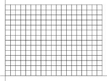
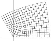
Figure 1. Domain (left) and image (right) for the discrete power function $z^{4/3}$.

2.3. Discrete minimal surfaces

The representation (2.1) for smooth minimal surfaces above suggests that the definition for discrete minimal surfaces is (see [14])

(2.5) $$f_{q}-f_{p}=(i-g_{p}j)j\frac{\alpha_{pq}}{g_{q}-g_{p}}(i-g_{q}j)\;,$$

where $g:D\to\mathbb{C}$ is a discrete holomorphic function with cross ratio factorizing function $\alpha$, and $p$ and $q$ are either $(m,n)$ and $(m+1,n)$, or $(m,n)$ and $(m,n+1)$. This defines the surface $f$ up to translations of $\mathbb{R}^{3}$. The freedom of scaling of $\alpha$ leads to homotheties of $f$.

As in the smooth case, where we avoided umbilics, and thus $g^{\prime}$ was never zero, we will make the following assumption throughout this paper:

$$\text{Assumption:}\;\;\;g_{q}-g_{p}\neq 0\;.$$

Example 2.1.

The discrete holomorphic function $c(m+in)$ for $c$ a complex constant will produce a minimal surface called a discrete Enneper surface, and graphics for this surface can be seen in [7].

Example 2.2.

The discrete holomorphic function $e^{c_{1}m+ic_{2}n}$ for choices of constants $c_{1}$ and $c_{2}$ so that the cross ratio is identically $-1$ will produce a minimal surface called a discrete catenoid, and graphics for this surface also can be seen in [7].

3. Smooth CMC $1$ surfaces, flat fronts, and linear Weingarten surfaces in $\mathbb{H}^{3}$

3.1. Smooth CMC $1$ surfaces

Similarly to the case of minimal surfaces, we can describe smooth and discrete CMC $1$ surfaces in $\mathbb{H}^{3}$. Hyperbolic $3$-space $\mathbb{H}^{3}$, considered in Minkowski $4$-space $\mathbb{R}^{3,1}=\{(x_{0},x_{1},x_{2},x_{3})\,|\,x_{j}\in\mathbb{R}\}$ (with Minkowski metric $-dx_{0}^{2}+dx_{1}^{2}+dx_{2}^{2}+dx_{3}^{2}$), is

$$\mathbb{H}^{3}=\{(x_{0},x_{1},x_{2},x_{3})\in\mathbb{R}^{3,1}\,|\,x_{0}>0,x_{0}^{2}-x_{1}^{2}-x_{2}^{2}-x_{3}^{2}=1\}\approx$$

$$\left\{\left.X=\begin{pmatrix}x_{0}+x_{3}&x_{1}+ix_{2}\\ x_{1}-ix_{2}&x_{0}-x_{3}\end{pmatrix}\right|\,\text{tr}(X)>0,\det X=1\right\}=\{F\cdot\bar{F}^{T}\,|\,F\in SL_{2}(\mathbb{C})\}\;,$$

where the superscript $T$ denotes transposition.

A smooth isothermically-parametrized CMC $1$ surface (away from umbilic points), has the Bryant equation [11]

(3.1) $$dF=F\begin{pmatrix}g&-g^{2}\\ 1&-g\end{pmatrix}\frac{dz}{g^{\prime}}\;,\;\;\;F\in SL_{2}(\mathbb{C})\;,$$

where $g$ is a holomorphic function with nonzero derivative, and the surface is then

$$f_{1}=F\cdot\bar{F}^{T}\in\mathbb{H}^{3}\;.$$

3.2. Smooth flat fronts

Starting with a smooth CMC $1$ surface $f_{1}$ with lift $F$ as above, define

(3.2) $$E=F\cdot\begin{pmatrix}1&g\\ 0&1\end{pmatrix}\;.$$

A flat front is then given by

$$f_{0}=E\cdot\bar{E}^{T}\in\mathbb{H}^{3}\;,$$

with unit normal vector field

(3.3) $$N=E\cdot\begin{pmatrix}1&0\\ 0&-1\end{pmatrix}\cdot\bar{E}^{T}\;.$$

We know this surface $f_{0}$ is flat, because (see [13])

(3.4) $$dE=E\begin{pmatrix}0&g^{\prime}\\ (g^{\prime})^{-1}&0\end{pmatrix}dz\;.$$

This surface with singularities is actually a front, because $|g^{\prime}|^{2}+|g^{\prime}|^{-2}>0$, which means that the associated Sasakian metric is positive definite. (See Theorem 2.9 in [22].) The notion of fronts is important in the study of smooth flat surfaces with singularities in $\mathbb{H}^{3}$. For example, it is a necessary notion for considering the caustic of a flat surface with singularities. However, it will not play such a direct role in our considerations on discrete surfaces here. Thus, from here on out, we will simply consider smooth flat surfaces with singularities, and sometimes will even just call them flat surfaces even though they might have singularities. When the front property is actually playing a role, we shall parenthetically refer to the word ”front”. For more information about flat fronts, see [18], [19] and [22].

Remark 3.1.

Because the off-diagonal terms $g^{\prime}$ and $(g^{\prime})^{-1}$ in (3.4) are inverse to each other, the conditions in [18] for having singular points, cuspidal edges and swallowtails on $f_{0}$ simplify to this:

1. singular points occur precisely at points where $|g^{\prime}|=1$;

2. a singular point is a cuspidal edge if and only if $\text{Im}(\tfrac{g^{\prime\prime}}{g^{\prime}})\neq 0$ (”Re” and ”Im” denote the real and imaginary parts, respectively);

3. a singular point is a swallowtail if and only if $g^{\prime\prime}\neq 0$ and $\text{Im}(\tfrac{g^{\prime\prime}}{g^{\prime}})=0$ and $\text{Re}((\tfrac{g^{\prime\prime}}{g^{\prime}})^{\prime})\neq 0$.

The condition that $\text{Im}(\tfrac{g^{\prime\prime}}{g^{\prime}})=0$ holds at some point along a singular curve $|g^{\prime}|=1$ is equivalent to the curve having a vertical tangent line at that point.

3.3. The hyperbolic Schwarz map and a special coordinate $w$

For later reference, we can take a new coordinate $w$ such that

$$dw=\frac{1}{g^{\prime}}dz\;,$$

which is locally well-defined, and still conformal, although not necessarily isothermic. This gives

(3.5) $$E^{-1}dE=\begin{pmatrix}0&q\\ 1&0\end{pmatrix}dw\;,$$

with

$$q|_{w(z)}=(g^{\prime})^{2}=\left.\frac{dg}{dw}\right|_{w(z)}\;.$$

The reason for changing variables from $z$ to $w$ is that Equation (3.5) now becomes

(3.6) $$\tfrac{d^{2}}{dw^{2}}u-q(w)\cdot u=0$$

with $f_{0}=E\bar{E}^{T}$ the hyperbolic Schwarz map (see [28]), where

(3.7) $$E=\begin{pmatrix}u_{1}&\tfrac{d}{dw}u_{1}\\ u_{2}&\tfrac{d}{dw}u_{2}\end{pmatrix}\;,$$

with functions $u_{1}$, $u_{2}$ that are linearly independent solutions of Equation (3.6) chosen so that the constant $u_{1}\tfrac{d}{dw}(u_{2})-u_{2}\tfrac{d}{dw}(u_{1})$ will be $1$. This equation (3.6) with $q(w)=w$ is the well-known Airy equation.

Remark 3.2.

Using $q$ and $w$, the conditions in Remark 3.1 become:

1. Singular points: $|q|=1$,

2. Cuspidal edge points: $\text{Im}(\tfrac{q_{w}}{q^{3/2}})\neq 0$,

3. Swallowtail points: $q_{w}\neq 0$, $\text{Im}(\tfrac{q_{w}}{q^{3/2}})=0$ and $\text{Re}(\tfrac{2q_{ww}q-3q_{w}^{2}}{q^{3}})\neq 0$.

3.4. Smooth linear Weingarten surfaces of Bryant type

We will now give a deformation through linear Weingarten surfaces between the surfaces $f_{1}$ and $f_{0}$ described in Sections 3.1 and 3.2. This deformation was first introduced in [13]. There are numerous ways to choose the deformation, and no one way is geometrically more canonical than any other. We will soon come back to this issue (Section 3.5). However, for now we will simply fix one choice for the deformation – the one that deforms the $f_{1}$ and $f_{0}$ as given in Sections 3.1 and 3.2 into each other, in accordance with the notations of previous papers ([18], [19], [20], [22]).

This particular choice will suffice when we switch to investigating discrete surfaces later. In fact, the resulting classes of discrete flat surfaces and discrete linear Weingarten surfaces of Bryant type, although defined in terms of the deformation, do not actually depend on the choice of deformation. (We say more about this in Section 4.4.) Hence the theorems we prove about these surfaces also are independent of the choice of deformation.

We shall refer to this choice of deformation as the ”first Weingarten family” (of either $f_{1}$ or $f_{0}$), and the procedure that we follow for constructing it is as follows. Following [13],

• we convert the $E$ in [13], actually notated as “$g$” there, to $(E^{T})^{-1}$,

• then changing the holomorphic function $h$ in [13] to $-g$ for the function $g$ given here,

• and allowing $-\omega$ in [13] to become $dz/g^{\prime}$ for the function $g$ here,

• and also changing $f$ and $N$ to $(f^{T})^{-1}$ and $(N^{T})^{-1}$, respectively,

a linear Weingarten surface of Bryant type in $\mathbb{H}^{3}$ satisfying (see also [21])

(3.8) $$2t(H-1)+(1-t)K=0\;,$$

where $H$ and $K$ are the mean and intrinsic curvatures, respectively, is

$$f_{t}=(EL)\overline{(EL)}^{T}\;.$$

Here $E$ satisfies (3.4) and

$$L=\begin{pmatrix}\beta&-tg\beta\\ 0&\beta^{-1}\end{pmatrix}\;,\;\;\;\beta=\sqrt{\frac{1+tg\bar{g}}{1+t^{2}g\bar{g}}}\in\mathbb{R}\;.$$

All linear Weingarten surfaces satisfying (3.8) (i.e. of Bryant type) can be constructed in this way (see [13]).

When $t=0$, we use the frame $E=E\cdot(L|_{t=0})=F\cdot\begin{pmatrix}1&g\\ 0&1\end{pmatrix}$, giving a flat surface $f_{0}$, as in Section 3.2. When $t=1$, we use the frame $F=E\cdot(L|_{t=1})=E\cdot\begin{pmatrix}1&-g\\ 0&1\end{pmatrix}$, giving a CMC $1$ surface $f_{1}$, as in Section 3.1. Thus we have a deformation through linear Weingarten surfaces in $\mathbb{H}^{3}$, from CMC $1$ surfaces in $\mathbb{H}^{3}$ to flat surfaces in $\mathbb{H}^{3}$. (See also [21].)

3.5. Geometric non-uniqueness of the deformation in [13]

We now explain in more detail why there is non-uniqueness for the choice of deformation through linear Weingarten surfaces of Bryant type. The deformation between smooth flat surfaces and smooth CMC $1$ surfaces through linear Weingarten surfaces, given in Section 3.4, is not uniquely determined in any geometric sense, because of ambiguities in the choice of Weierstrass data. We illustrate this with two lemmas, both of which are easily verified:

Lemma 3.3.

Given a smooth isothermically-parametrized CMC $1$ surface $f_{1}$ in $\mathbb{H}^{3}$ with lift $F$ and Weierstrass data $g$, the transformation

$$F\to F\cdot B\;,\;\;\;B=\begin{pmatrix}p&q\\ -\bar{q}&\bar{p}\end{pmatrix}\in\text{SU}_{2}$$

will not change the resulting surface $f_{1}=F\cdot\bar{F}^{T}=FB\cdot\overline{FB}^{T}$, and will change the Weierstrass data by

$$g\to\hat{g}=\frac{\bar{p}g-q}{\bar{q}g+p}\;.$$

Remark 3.4.

By Lemma 3.3, different choices for $B$ do not affect $f_{1}$. However, when $B$ is not diagonal, the transformation in the above lemma generally will result in a different deformation $f_{t}$ through linear Weingarten surfaces for $t<1$, and also in a different flat surface $f_{0}$.

Lemma 3.5.

Given a flat surface $f_{0}$ with Weierstrass data $g^{\prime}$ and lift $E$ as in Equation (3.4), then the transformation

$$g\to g+a\;,$$

followed by the transformation

$$E\to E\cdot B\;,$$

where $B\in\text{SU}_{2}$ is either diagonal or off-diagonal and $a$ is any complex constant, will not change the resulting surface $f_{0}=E\cdot\bar{E}^{T}=EB\cdot\overline{EB}^{T}$.

Remark 3.6.

Under the transformations of $E$ and $g$ in Lemma 3.5, $f_{0}$ is not affected. However, when $B$ is off-diagonal or $a$ is not zero, these transformations generally will result in a different deformation $f_{t}$ through linear Weingarten surfaces for $t>0$. In particular, the CMC $1$ surface $f_{1}$ generally will change.

The two lemmas and two remarks above show that the ”first Weingarten family” deformation will change when different Weierstrass data is used, even when the original surface under consideration does not change.

To demonstrate that other choices actually do give different deformations, we will also consider a deformation we call the ”second Weingarten family”, given by starting with a flat surface $f_{0}$ with given lift $E$, and then using the lift $EB$ for an off-diagonal $B\in\text{SU}_{2}$ instead to make the deformation through linear Weingarten surfaces of Bryant type. (Any choice of off-diagonal $B\in\text{SU}_{2}$ will result in the same deformation.) Regardless of whether $E$ or $EB$ is used, we have the same surface $f_{0}$, but $E$ and $EB$ give opposite orientations for the normal vector to $f_{0}$, and we are interested in this particular choice for a second deformation precisely because of this orientation-reversing property. The frames $E$ and $EB$ give different families of linear Weingarten surfaces when $t>0$. Such different deformations of surfaces can be seen in Figures 2 (first Weingarten family) and 3 (second Weingarten family), and also in Figures 5 (first Weingarten family) and 6 (second Weingarten family).

3.6. The deformations with respect to the coordinate $w$

The first Weingarten family is

$$f_{t}^{(1)}=(EL)(\overline{EL})^{T}\;,$$

where $L$ is as in Section 3.4 and $E$ solves Equation (3.4). In terms of the new coordinate $w$ given in Section 3.3, since $g=\int qdw$, $L$ takes the form

$$L=\begin{pmatrix}\beta&-t\beta\cdot\int qdw\\ 0&\beta^{-1}\end{pmatrix}\;,\;\;\;\beta=\beta(w)=\sqrt{\frac{1+t|\int qdw|^{2}}{1+t^{2}|\int qdw|^{2}}}\;.$$

A second Weingarten family $f_{t}^{(2)}$ can be given by taking

$$B=\begin{pmatrix}0&1\\ -1&0\end{pmatrix}\;,$$

and then

$$f_{t}^{(2)}=EB\hat{L}(\overline{EB\hat{L}})^{T}\;,$$

where

$$\hat{L}=\begin{pmatrix}\hat{\beta}&-th\hat{\beta}\\ 0&\hat{\beta}^{-1}\end{pmatrix}\;,\;\;\;\hat{\beta}=\sqrt{\frac{1+th\bar{h}}{1+t^{2}h\bar{h}}}\;,\;\;\;h=\int\frac{-1}{g^{\prime}}dz\;,$$

and $E$ again solves (3.4). Note that there is freedom of choice of additive constant in the definition of $h$, and different constants will give different deformations.

In terms of the new coordinate $w$ satisfying $dw=\frac{1}{g^{\prime}}dz$ (and $q=(g^{\prime})^{2}$) given in Section 3.3, a second Weingarten family $f^{(2)}_{t}$ has a particularly nice expression for its singular set:

Lemma 3.7.

The second Weingarten family $f^{(2)}_{t}$ taken by choosing $h=-w$ is singular along the curve

$$|q|^{2}(1+t|w|^{2})^{4}-(1-t)^{2}=0\;.$$

Note that, in particular, $f^{(2)}_{1}$ could be singular only at points where $q=0$.

Proof.

Note that

$$(EB)^{-1}d(EB)=-\begin{pmatrix}0&1\\ q&0\end{pmatrix}dw$$

and

$$f_{t}^{(2)}=\begin{pmatrix}x_{0}+x_{3}&x_{1}+ix_{2}\\ x_{1}-ix_{2}&x_{0}-x_{3}\end{pmatrix}=EB\begin{pmatrix}\tfrac{1+t^{2}|w|^{2}}{1+t|w|^{2}}&-t\bar{w}\\ -tw&1+t|w|^{2}\end{pmatrix}\bar{B}^{T}\bar{E}^{T}\;,$$

where the $x_{j}$ are now considered as real-valued functions of $w$ and $\bar{w}$ (and also of $t$). Substituting $dx_{k}=\tfrac{\partial x_{k}}{\partial w}dw+\tfrac{\partial x_{k}}{\partial\bar{w}}d\bar{w}$ into the Minkowski norm $dx_{1}^{2}+dx_{2}^{2}+dx_{3}^{2}-dx_{0}^{2}$, we find that

$${\mathfrak{A}}dw^{2}+\bar{\mathfrak{A}}d\bar{w}^{2}+2{\mathfrak{B}}dwd\bar{w}=dx_{1}^{2}+dx_{2}^{2}+dx_{3}^{2}-dx_{0}^{2}$$

has discriminant

$${\mathfrak{B}}^{2}-{\mathfrak{A}}\bar{\mathfrak{A}}=|u_{1}\tfrac{d}{dw}(u_{2})-u_{2}\tfrac{d}{dw}(u_{1})|^{4}\left(|q|^{2}(1+t|w|^{2})^{4}-(1-t)^{2}\right)^{2}(1+t|w|^{2})^{-4}\geq 0\;,$$

where $u_{1}$ and $u_{2}$ are as in Section 3.3. Since $u_{1}\tfrac{d}{dw}(u_{2})-u_{2}\tfrac{d}{dw}(u_{1})=1$, the proof is completed. ∎

3.7. Examples

We now give some examples.

Example 3.8.

Take any constant $q\in\mathbb{C}\setminus\{0\}$ in Equation (3.5). Then we can take $g=\sqrt{q}z=qw$, and so both the coordinates $z$ and $w$ will be isothermic if $q\in\mathbb{R}$, and we now assume $q$ is a positive real. Let us use the coordinate $w$, and then $E$ as in Section 3.3 can be taken as

$$E=q^{-1/4}\cdot\begin{pmatrix}\cosh(\sqrt{q}w)&\sqrt{q}\sinh(\sqrt{q}w)\\ \sinh(\sqrt{q}w)&\sqrt{q}\cosh(\sqrt{q}w)\end{pmatrix}$$

and we can take $F$ as

$$F=q^{-1/4}\cdot\begin{pmatrix}\cosh(\sqrt{q}w)&\sqrt{q}\sinh(\sqrt{q}w)-qw\cosh(\sqrt{q}w)\\ \sinh(\sqrt{q}w)&\sqrt{q}\cosh(\sqrt{q}w)-qw\sinh(\sqrt{q}w)\end{pmatrix}\;.$$

Then $f_{0}=E\bar{E}^{T}$ is a (geodesic) line when $|q|=1$, and is a (hyperbolic) cylinder when $|q|\neq 1$. Also, $f_{1}=F\bar{F}^{T}$ gives CMC $1$ Enneper cousins in $\mathbb{H}^{3}$ [11] [27] (see Figure 2). These $f_{1}$ and $f_{0}$ deform to each other via the first Weingarten family.

Now, consider half-lines in the domain (the complex plane $\mathbb{C}$) of the Enneper cousins $f_{1}$ emanating from the point $w=0$. In all but two directions for these rays, the corresponding curve on the surface will converge to a single point in the sphere at infinity $\partial\mathbb{H}^{3}$. This limit point can be different for different directions, and in particular the limit will be one certain point (resp. one other certain point) for any ray that makes an angle of less than (resp. more than) $\pi/2$ with the positive real axis in the $w$-plane. However, in the two special directions for these rays where $w$ is pure imaginary, the corresponding two curves on the surface converge to infinite wrappings of circles in $\partial\mathbb{H}^{3}$. These properties are easily checked, because we have an explicit form for $F$, as above. Furthermore, the behavior is the same for any $f_{t}^{(1)}$ whenever $t>0$, which is also easily checked. This behavior is similar to the Stokes phenomenon we will see in Example 3.10.

See Figure 2 for the first Weingarten family of $f_{0}$, and Figure 3 for a second Weingarten family of $f_{0}$.

Example 3.9.

To make CMC $1$ surfaces of revolution $f_{1}$, the so-called catenoid cousins [11] [32], one can use $g=e^{\mu z}$ in (3.1), for $\mu$ either real or purely imaginary. For the corresponding flat surfaces $f_{0}$, one can obtain the surfaces called hourglasses (resp. snowmen) by choosing real (resp. imaginary) values for $\mu$ [12] [22]. Discrete versions of these flat surfaces can be seen in Figure 7, and graphics of the smooth surfaces look much the same, but are smooth.

Example 3.10.

We will now consider the holomorphic function $g=z^{\gamma}=z^{4/3}$, which gives the hyperbolic Schwarz map $f_{0}$ for the Airy equation $\tfrac{d^{2}}{dw^{2}}u-wu=0$ as in Equation (3.6).

The value $\gamma=\tfrac{4}{3}$ corresponds to the choice $q=w$, and so is of particular interest. We can see this correspondence as follows: We take $q$ to be $w$. This means we have $w=(g^{\prime})^{2}$, and so $dw=2g^{\prime}g^{\prime\prime}dz$. Then, because $dw=(1/(dg/dz))dz$, we have $(1/(dg/dz))dz=2g^{\prime}g^{\prime\prime}dz$, and so the original holomorphic function $g$, as a function of $z$, would satisfy

$$\frac{1}{2}=g^{\prime\prime}(g^{\prime})^{2}$$

and so

$$g=\sqrt[3]{\tfrac{81}{128}}z^{4/3}\;,$$

and the scalar factor $\sqrt[3]{\tfrac{81}{128}}$ can be removed by replacing $z$ with an appropriate constant real multiple of $z$.

This surface $f_{0}$ has an umbilic point at $w=0$ (so the corresponding caustic will blow out to infinity at $w=0$, see [18], [19], [26]), and it has a ”triangle” of singular points with three cuspidal edge arcs connected by three swallowtail singularities, and it has $120$ degree dihedral symmetry. Similar to the case of the CMC $1$ Enneper cousins, starting at the center point of the surface ($w=0$ in the domain of the mapping) and going in any direction but three (i.e. following a ray out from $w=0$ in the domain), the corresponding curve on the surface will converge to a single point (one of three possible points) in the sphere at infinity $\partial\mathbb{H}^{3}$ (as in Example 3.8, this limit point can be different for different directions). However, in three special directions for these rays, the corresponding curves on the surface converge to infinite wrappings of circles in $\partial\mathbb{H}^{3}$. These special directions are exactly opposite to the directions of the swallowtail singularities. This is called Stokes phenomenon, and was explored carefully for this example in [28], [30]. Portions of this $f_{0}$ can be seen in Figure 4.

The surfaces $f_{t}^{(2)}$ ($0\leq t<1$) in a second Weingarten family of $f_{0}$ have the same property that the singular set is a triangle of three cuspidal edge arcs connected by three swallowtails. Then, as $t$ tends to $1$, the three swallowtails converge to the origin $w=0$, and when $t=1$ the CMC $1$ surface $f_{1}$ has a branch point of order $2$ at $w=0$. The deformation near the origin can be simulated by the map $Y_{s}:(u,v)\mapsto(y_{1},y_{2},y_{3})$ given by

$$y_{1}=-s(u^{2}+v^{2})+2uv^{2}-\tfrac{2}{3}u^{3}\;,\;\;\;y_{2}=2su+u^{2}-v^{2}\;,\;\;\;y_{3}=-sv+uv\;,$$

as $s=1-t$ tends to zero.

The first and second Weingarten families for $f_{0}$ can be seen in Figures 5 and 6.

More generally, using $q=w^{n}$ in (3.1) will give the flat surfaces $f_{0}$ investigated in [28]. When $n$ is neither $-1$ nor $-2$, we have $g=c_{n}z^{\frac{2n+2}{n+2}}$ for some $c_{n}>0$. When $q=w^{-1}$, then $g=2\log z$. When $q=w^{-2}$, we have $g=ce^{-z}$, and $c$ can take on any value.

Remark 3.11.

It is interesting to note that, in Example 3.10, while the two choices $q=w$ and $\hat{q}=\hat{w}^{-1/2}$ give different equations $\tfrac{d^{2}}{dw^{2}}u=wu$ and $\tfrac{d^{2}}{d\hat{w}^{2}}\hat{u}=\hat{w}^{-1/2}\hat{u}$, the solutions $\hat{u}$ to the second equation are essentially just $w$-derivatives of the solutions $u$ to the first equation. A computation then shows $q$ and $\hat{q}$ can produce two flat surfaces that are parallel surfaces of each other. In terms of the coordinate $z$, the corresponding statement is that $g=z^{4/3}$ and $\hat{g}=\hat{z}^{2/3}$ can produce two flat surfaces that are parallel to each other, and in fact this also follows from Lemma 3.5 (taking $B$ to be off-diagonal with off-diagonal entries both $i$).

$t=0$	$t=1/4$	$t=1/2$
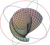
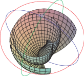
$t=3/4$	$t=1$

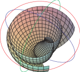
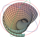
Figure 2. The first Weingarten family associated with a hyperbolic cylinder, in the Poincare ball model for $\mathbb{H}^{3}$. Here we take $q>0$ constant, so that $g^{\prime}=\sqrt{q}$ and $g=qw$. Half of each of the surfaces is cut away. Note that the surface is a CMC $1$ Enneper cousin when $t=1$. See Example 3.8. (Here we have included grid lines on these smooth surfaces simply to make the graphics more visible.)

$t=0$	$t=1/4$	$t=1/2$
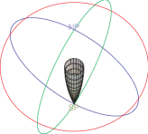
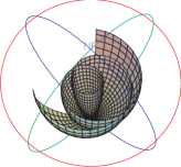
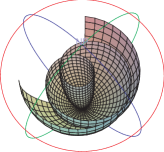
$t=3/4$	$t=1$

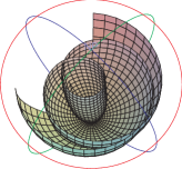
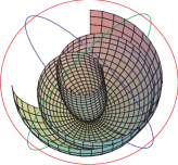
Figure 3. A second Weingarten family associated with a hyperbolic cylinder, in the Poincare ball model. See Example 3.8.

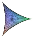
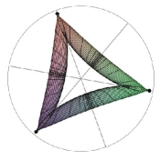
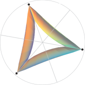
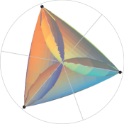
Figure 4. Images of the smooth flat surface related to the Airy equation $\frac{d^{2}}{dw^{2}}u-wu=0$, in the Poincare ball model. The left figure is the image of the unit disc $\{|w|\leq 1\}$, shown with grid lines for better visibility. The boundary of this left figure is the cuspidal edge curve with three swallowtail corners. The middle two figures are the image of the ring $\{1.17\leq w\leq 2.34\}$, shown twice, once with grid lines and once without. The right figure is the image of $\{3.27\leq w\leq 4.09\}$, this time shown without grid lines because in this case visibility is better without them. See Example 3.10.

$t=0$ (flat)	$t=1/2$
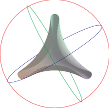
$t=1$ (CMC 1)	$t=1$ (CMC 1)

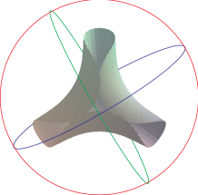
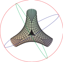
Figure 5. The first Weingarten family associated with the Airy equation, in the Poincare ball model. See Example 3.10. The bottom two figures are the same CMC $1$ surface, shown once with grid lines and once without.

$t=0$ (flat)	$t=1/10$
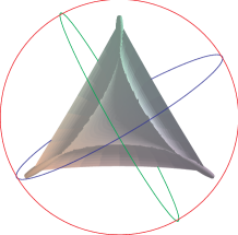
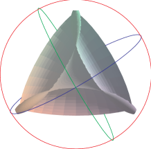
$t=1/2$	$t=1$ (CMC 1)	$t=1$ (CMC 1)

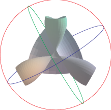
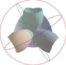
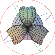
Figure 6. A second Weingarten family associated with the Airy equation, in the Poincare ball model. See Example 3.10. The two lower-right figures are the same CMC $1$ surface, shown once with grid lines and once without. (The upper-left surface here is the same as the upper-left surface in Figure 5.)

4. Discrete CMC $1$, flat and linear Weingarten surfaces in $\mathbb{H}^{3}$

4.1. Known definition for discrete CMC $1$ surfaces

We now describe how discrete CMC $1$ surfaces in $\mathbb{H}^{3}$ were defined in [14]. For this, we first give a light cone model for $\mathbb{H}^{3}$ in Minkowski $5$-space $\mathbb{R}^{4,1}$ that is commonly used in Moebius geometry, and that was used in [14] in conjunction with quaternions. Let $\mathcal{H}$ denote the $4$-dimensional vector space of quaternions with the usual basis $1$, $i$, $j$ and $k$, and with the usual notion of quaternionic multiplication. Points $(x_{1},x_{2},x_{3},x_{4},x_{0})\in\mathbb{R}^{4,1}$ can then be given by

(4.1) $$X=x_{1}\begin{pmatrix}i&0\\ 0&-i\end{pmatrix}+x_{2}\begin{pmatrix}j&0\\ 0&-j\end{pmatrix}+x_{3}\begin{pmatrix}k&0\\ 0&-k\end{pmatrix}+x_{4}\begin{pmatrix}0&1\\ -1&0\end{pmatrix}+x_{0}\begin{pmatrix}0&1\\ 1&0\end{pmatrix}\;,$$

and the $\mathbb{R}^{4,1}$ metric $\langle X,X\rangle$ is then given by ($I$ is the identity matrix)

$$\langle X,X\rangle\cdot I=-X^{2}\;.$$

Now let us view the collection of such trace-free $2\times 2$ matrices with imaginary quaternions on the diagonal and reals on the off-diagonal as the set of points in $\mathbb{R}^{4,1}$. We can then define $\mathbb{H}^{3}$ as a $3$-dimensional submanifold of the light cone in this way:

(4.2) $$\mathbb{H}^{3}=\left\{X\in\mathbb{R}^{4,1}\,\left|\,X^{2}=0,X\cdot\begin{pmatrix}-i&0\\ 0&i\end{pmatrix}+\begin{pmatrix}-i&0\\ 0&i\end{pmatrix}\cdot X=2I\right.\right\}\;.$$

This $\mathbb{H}^{3}$ will have constant sectional curvature $-1$ when given the induced metric from $\mathbb{R}^{4,1}$. Furthermore, for each point $X$ in the light cone, there is at most one value for $r\in\mathbb{R}$ so that $rX$ lies in $\mathbb{H}^{3}$, so we can alternately view $\mathbb{H}^{3}$ as the projectivized light cone.

In [14], in order to define discrete CMC $1$ surfaces in $\mathbb{H}^{3}$, the discrete version of the Bryant equation

(4.3) $$F_{q}-F_{p}=F_{p}\begin{pmatrix}g_{p}&-g_{p}g_{q}\\ 1&-g_{q}\end{pmatrix}\frac{\lambda\alpha_{pq}}{g_{q}-g_{p}}\;,\;\;\;\det F\in\mathbb{R}\;,$$

was used, where $g$ is a discrete holomorphic function with cross ratio factorizing function $\alpha_{pq}$, and $p$ and $q$ are adjacent vertices in the domain $D\subset\mathbb{Z}^{2}$ of $g$. Note that we have assumed $g_{q}-g_{p}\neq 0$ (see Section 2.3). The nonzero real parameter $\lambda$ can be chosen freely. The formula for the discrete CMC $1$ surface $f$ in $\mathbb{H}^{3}$ was then obtained, analogous to the formula (2.5) for the case of discrete minimal surfaces, by setting (here $\mathbb{L}^{4}$ is the $4$-dimensional light cone in $\mathbb{R}^{4,1}$)

(4.4) $$f_{1,p}=r\cdot\begin{pmatrix}-b\bar{a}&a\bar{a}\\ b\bar{b}&-a\bar{b}\end{pmatrix}\in\mathbb{H}^{3}\subset\mathbb{L}^{4}\subset\mathbb{R}^{4,1}\;,\;\;\;\text{where}\;\;\begin{pmatrix}a\\ b\end{pmatrix}=\begin{pmatrix}0&1\\ j&0\end{pmatrix}F_{p}\begin{pmatrix}i\\ j\end{pmatrix}\;,$$

where $r$ is the appropriate choice of real scalar to place $f_{1,p}$ in $\mathbb{H}^{3}$ as defined in (4.2). In fact,

$$r=2(b\bar{a}i+ib\bar{a})^{-1}=-2(a\bar{b}i+ia\bar{b})^{-1}\in\mathbb{R}\;.$$

Because the entries of $F$ are complex, not quaternionic, it follows that $b\bar{a}$ is purely imaginary quaternionic, so the above matrix $f_{1,p}$ does lie in $\mathbb{R}^{4,1}$, and thus in $\mathbb{L}^{4}$ and then also in $\mathbb{H}^{3}$ with appropriate choice of $r$. Also, we actually have a $1$-parameter family of surfaces, due to the freedom of choice of $\lambda$.

The solution $F$ is defined only up to scalar factors. This is essentially because Equation (4.3) is not symmetric in $p$ and $q$, and can be explained as follows: Consider a quadrilateral in $D$ with vertices $p$, $q$, $r$ and $s$ given counterclockwise about the quadrilateral, and with $p$ as the lower left vertex. Then $F_{q}=F_{p}\cdot\mathfrak{A}$ with $\mathfrak{A}$ determined by Equation (4.3). Then $F_{r}=F_{q}\cdot\mathfrak{B}$, again by (4.3). Similarly, $F_{s}=F_{p}\cdot\mathfrak{C}$ and $F_{r}=F_{s}\cdot\mathfrak{D}$. Thus we expect $\mathfrak{A}\mathfrak{B}=\mathfrak{C}\mathfrak{D}$, and a computation shows that this is indeed the case. However, we also have $F_{p}$ equal to $F_{q}\cdot\hat{\mathfrak{A}}$, by (4.3) with the roles of $p$ and $q$ reversed, and it turns out that $\mathfrak{A}\hat{\mathfrak{A}}=(1-\lambda\alpha_{pq})I\neq I$. Thus, the solution $F$ to (4.3) is only defined projectively, that is, it is only defined up to scalar factors.

Nevertheless, because we are scaling by a real factor $r$ in Equation (4.4) anyways, the resulting discrete CMC $1$ surface is still well-defined. Thus we have seen the following lemma.

Lemma 4.1.

Although the solution $F$ of Equation (4.3) is multi-valued and only defined up to scalar factors, the discrete CMC $1$ surface $f_{1}$ given in (4.4) is well-defined.

In fact, the upcoming Theorem 4.2 also implies that the discrete CMC $1$ surface $f_{1}$ is well-defined.

4.2. New formulation for discrete CMC $1$ surfaces

Equivalently to the definition given in [14], there is another way to define $f_{p}$, which is given in the next theorem. This new form for $f_{p}$ is convenient, because it is clearly analogous to the form used in the Bryant representation for smooth CMC $1$ surfaces in $\mathbb{H}^{3}$, and it removes the need for the Moebius-geometric $\mathbb{R}^{4,1}$ light cone model for $\mathbb{H}^{3}$.

Theorem 4.2.

The above description (4.4) for the discrete CMC $1$ surface given by $F$ is equal to the surface given by $\frac{1}{\det F}F\bar{F}^{T}$, up to a rigid motion of $\mathbb{H}^{3}$.

Proof.

The matrices $f_{p}$ in $\mathbb{H}^{3}$, as described in (4.4), will be of the form

$$r\begin{pmatrix}-(\bar{A}C+\bar{B}D)j+i(AD-BC)&C\bar{C}+D\bar{D}\\ A\bar{A}+B\bar{B}&j(A\bar{C}+B\bar{D})-i(AD-BC)\end{pmatrix}\;,$$

where $r$ is a nonzero real scalar and

$$F=\begin{pmatrix}A&B\\ C&D\end{pmatrix}\;.$$

To have $f_{1,p}\in\mathbb{H}^{3}$, we should take

$$r=\frac{1}{AD-BC}\;.$$

This means that the coefficient of the $i$ term in the diagonal entries will be simply $\pm 1$. So we can view the surface as lying in the $4$-dimensional space $\mathbb{R}^{3,1}$, by simply removing the matrix term with scalar $x_{1}$ from Equation (4.1).

Now, the projection into the Poincare ball model is

$$(x_{2},x_{3},x_{4},x_{0})\to\frac{(x_{2},x_{3},x_{4})}{1+x_{0}}=$$

(4.5) $$\frac{(\text{Re}(-\bar{A}C-\bar{B}D),\text{Im}(-\bar{A}C-\bar{B}D),\tfrac{1}{2}(-A\bar{A}-B\bar{B}+C\bar{C}+D\bar{D}))}{AD-BC+\tfrac{1}{2}(A\bar{A}+B\bar{B}+C\bar{C}+D\bar{D})}\;.$$

On the other hand, if we look at

$$\frac{1}{AD-BC}F\bar{F}^{T}=\frac{1}{AD-BC}\begin{pmatrix}A\bar{A}+B\bar{B}&A\bar{C}+B\bar{D}\\ C\bar{A}+D\bar{B}&C\bar{C}+D\bar{D}\end{pmatrix}=\begin{pmatrix}y_{0}+y_{3}&y_{1}+iy_{2}\\ y_{1}-iy_{2}&y_{0}-y_{3}\end{pmatrix}\;,$$

and then project to the Poincare ball, we have

$$\frac{(y_{1},y_{2},y_{3})}{1+y_{0}}=$$

(4.6) $$\frac{(\text{Re}(A\bar{C}+B\bar{D}),\text{Im}(A\bar{C}+B\bar{D}),\tfrac{1}{2}(A\bar{A}+B\bar{B}-C\bar{C}-D\bar{D}))}{AD-BC+\tfrac{1}{2}(A\bar{A}+B\bar{B}+C\bar{C}+D\bar{D})}\;.$$

The quantities (4.5) and (4.6) are the same, up to a rigid motion of $\mathbb{H}^{3}$, proving the theorem. ∎

4.3. Discrete flat surfaces

To make discrete flat surfaces in $\mathbb{H}^{3}$, we can now take

(4.7) $$E_{p}=F_{p}\cdot\begin{pmatrix}1&g_{p}\\ 0&1\end{pmatrix}\;,\;\;\;\det E=\det F\in\mathbb{R}\;,$$

like in (3.2) for the smooth case. We then use the same formula (4.4) as for discrete CMC $1$ surfaces to define the discrete flat surface, but with $F_{p}$ replaced by $E_{p}$. In light of Theorem 4.2, the following definition is natural:

Definition 4.3.

For $E$ given as in (4.7), where $F$ is a solution of Equation (4.3),

(4.8) $$f_{0}=\frac{1}{\det E}E\bar{E}^{T}$$

is a discrete flat surface.

Furthermore, in light of the behavior of the normal for smooth flat surfaces in Equation (3.3), it is natural to define the normal at vertices of a discrete flat surface by

(4.9) $$N_{p}:=\frac{1}{\det E_{p}}E_{p}\cdot\begin{pmatrix}1&0\\ 0&-1\end{pmatrix}\cdot\bar{E}_{p}^{T}\;.$$

A discrete version of Equation (3.4) can then be computed, and becomes

(4.10) $$E_{q}-E_{p}=E_{p}\begin{pmatrix}0&g_{q}-g_{p}\\ \frac{\lambda\alpha_{pq}}{g_{q}-g_{p}}&0\end{pmatrix}\;,$$

where $\lambda$ is an arbitrary parameter in $\mathbb{R}\setminus\{0\}$.

Remark 4.4.

Like in Lemma 4.1 for $F$, this $E$ is only defined up to scalar factors. However, the discrete flat surface $f_{0}$ is still well-defined.

Remark 4.5.

Changing $g_{p}$ to $d\cdot g_{p}$ for $d\in\mathbb{R}^{+}$ gives parallel discrete flat surfaces, and this is seen as follows: $g_{p}\to d\cdot g_{p}$ implies

(4.11) $$E_{p}\to E_{p}^{d}:=E_{p}\cdot\begin{pmatrix}1/\sqrt{d}&0\\ 0&\sqrt{d}\end{pmatrix}\;,$$

which implies the original surface $f_{0,p}=\tfrac{1}{\det E_{p}}E_{p}\bar{E}_{p}^{T}$ changes to

(4.12) $$f_{0,p}^{d}=\cosh(\log d)\,\cdot f_{0,p}-\sinh(\log d)\,\cdot N_{p}\;.$$

This surface $f_{0}^{d}$ is a parallel surface of $f_{0}$, and $f_{0}^{1}$ is the same as the original surface $f_{0}$. It also follows from (4.11) and (4.12) that the geodesic at $f_{0,p}$ in the direction $N_{p}$ and the geodesic at $f_{0,p}^{d}$ in the direction $N_{p}^{d}=\tfrac{1}{\det E_{p}^{d}}E_{p}^{d}\begin{pmatrix}1&0\\ 0&-1\end{pmatrix}\overline{E_{p}^{d}}^{T}$ are the same.

We now give one of our main results:

Theorem 4.6.

Discrete flat surfaces in $\mathbb{H}^{3}$ have concircular quadrilaterals.

Remark 4.7.

Although they have concircular quadrilaterals, discrete flat surfaces are generally not discrete isothermic. This is expected, since smooth flat surfaces given as in Section 3.2 are generally not isothermically parametrized as well.

Proof.

Let $f_{0}=\frac{1}{\det(E)}E\bar{E}^{T}$ be a discrete flat surface defined on a domain $D\subseteq\mathbb{Z}^{2}$, formed from a discrete holomorphic function $g$ on $D$. Let $p=(m,n)$, $q=(m+1,n)$, $r=(m+1,n+1)$ and $s=(m,n+1)$ be the vertices of one quadrilateral in $D$, and let $E_{p}$, $E_{q}$, $E_{r}$ and $E_{s}$ be the respective values of $E$ at those vertices. We choose a cross ratio factorizing function for $g$, and we denote that function’s value on the edge from $p$ to $q$, respectively $p$ to $s$, as $\alpha_{pq}$, respectively $\alpha_{ps}$. Then

$$\begin{array}[]{rcl}E_{q}=E_{p}U\;,\;\;\;\;\;U&=&\left(\begin{array}[]{cc}1&g_{q}-g_{p}\\ \frac{\lambda\alpha_{pq}}{g_{q}-g_{p}}&1\end{array}\right)\;,\\ E_{s}=E_{p}V\;,\;\;\;\;\;V&=&\left(\begin{array}[]{cc}1&g_{s}-g_{p}\\ \frac{\lambda\alpha_{ps}}{g_{s}-g_{p}}&1\end{array}\right)\;,\\ E_{r}=E_{p}UV_{1}=E_{p}VU_{1}\;,\;\;\;\;\;U_{1}&=&\left(\begin{array}[]{cc}1&g_{r}-g_{s}\\ \frac{\lambda\alpha_{pq}}{g_{r}-g_{s}}&1\end{array}\right)\;,\\ V_{1}&=&\left(\begin{array}[]{cc}1&g_{r}-g_{q}\\ \frac{\lambda\alpha_{ps}}{g_{r}-g_{q}}&1\end{array}\right)\end{array}$$

(note that we have $UV_{1}=VU_{1}$, by the cross ratio identity in Equation (2.2)).

Now the cross ratio for the quadrilateral given by the four surface vertices $f_{0,p}$, $f_{0,q}$, $f_{0,r}$ and $f_{0,s}$ is

$$C=(f_{0,p}-f_{0,q})(f_{0,q}-f_{0,r})^{-1}(f_{0,r}-f_{0,s})(f_{0,s}-f_{0,p})^{-1}\;,$$

or equivalently

$$(f_{0,p}-f_{0,q})(f_{0,q}-f_{0,r})^{-1}=C(f_{0,p}-f_{0,s})(f_{0,s}-f_{0,r})^{-1}\;.$$

(Note that commutativity does not hold for the product of four terms in this $C$, so it is vital that the order of the product be given correctly.) To prove the theorem, it suffices to show that $C$ is a real scalar factor times the identity matrix.

Note that

$$f_{0,p}-f_{0,q}=\frac{1}{\det(E_{p})}E_{p}(I-\frac{1}{\det(U)}U\bar{U}^{T})\bar{E}_{p}^{T}$$

and

$$f_{0,q}-f_{0,r}=\frac{1}{\det(E_{p})}\frac{1}{\det(U)}E_{p}U(I-\frac{1}{\det(V_{1})}V_{1}\bar{V}_{1}^{T})\bar{U}^{T}\bar{E}_{p}^{T}\;,$$

so we have

$$(f_{0,p}-f_{0,q})(f_{0,q}-f_{0,r})^{-1}=\det(U)E_{p}(I-\frac{1}{\det(U)}U\bar{U}^{T})(\bar{U}^{T})^{-1}(I-\frac{1}{\det(V_{1})}V_{1}\bar{V}_{1}^{T})^{-1}U^{-1}E_{p}^{-1}\;,$$

and likewise

$$(f_{0,p}-f_{0,s})(f_{0,s}-f_{0,r})^{-1}=\det(V)E_{p}(I-\frac{1}{\det(V)}V\bar{V}^{T})(\bar{V}^{T})^{-1}(I-\frac{1}{\det(U_{1})}U_{1}\bar{U}_{1}^{T})^{-1}V^{-1}E_{p}^{-1}\;.$$

So one finds that

$$\det(U_{1})E_{p}(\det(U)(\bar{U}^{T})^{-1}-U)(\det(V_{1})V_{1}^{-1}-\bar{V}_{1}^{T})^{-1}V_{1}^{-1}U^{-1}=$$

$$=\det(V_{1})CE_{p}(\det(V)(\bar{V}^{T})^{-1}-V)(\det(U_{1})U_{1}^{-1}-\bar{U}_{1}^{T})^{-1}U_{1}^{-1}V^{-1}\;.$$

Because $UV_{1}=VU_{1}$, we have

$$\frac{\det(U_{1})}{\det(V_{1})}E_{p}(\det(U)(\bar{U}^{T})^{-1}-U)(\det(V_{1})V_{1}^{-1}-\bar{V}_{1}^{T})^{-1}=$$

$$CE_{p}(\det(V)(\bar{V}^{T})^{-1}-V)(\det(U_{1})U_{1}^{-1}-\bar{U}_{1}^{T})^{-1}\;.$$

The determinants of $U$ and $V$ are real, so for example $\det(U)(\bar{U}^{T})^{-1}=\left(\begin{array}[]{cc}1&\frac{\lambda\alpha_{pq}}{\bar{g}_{p}-\bar{g}_{q}}\\ \bar{g}_{p}-\bar{g}_{q}&1\end{array}\right)$ and we get

$$\det(U)(\bar{U}^{T})^{-1}-U=(|g_{q}-g_{p}|^{2}+\lambda\alpha_{pq})\begin{pmatrix}0&\frac{1}{\bar{g}_{p}-\bar{g}_{q}}\\ \frac{1}{g_{p}-g_{q}}&0\end{pmatrix}\;.$$

With similar expressions for the other differences we see that

$$\frac{\det(U_{1})}{\det(V_{1})}\frac{|g_{q}-g_{p}|^{2}+\lambda\alpha_{pq}}{|g_{r}-g_{q}|^{2}+\lambda\alpha_{ps}}E_{p}\begin{pmatrix}0&\frac{1}{\bar{g}_{p}-\bar{g}_{q}}\\ \frac{1}{g_{p}-g_{q}}&0\end{pmatrix}\begin{pmatrix}0&g_{q}-g_{r}\\ \bar{g}_{q}-\bar{g}_{r}&0\end{pmatrix}=$$

$$=\frac{|g_{s}-g_{p}|^{2}+\lambda\alpha_{ps}}{|g_{r}-g_{s}|^{2}+\lambda\alpha_{pq}}CE_{p}\begin{pmatrix}0&\frac{1}{\bar{g}_{p}-\bar{g}_{s}}\\ \frac{1}{g_{p}-g_{s}}&0\end{pmatrix}\begin{pmatrix}0&g_{s}-g_{r}\\ \bar{g}_{s}-\bar{g}_{r}&0\end{pmatrix}\;.$$

So the expression for $C$ is

$$C=\mu E_{p}\begin{pmatrix}\frac{\bar{g}_{q}-\bar{g}_{r}}{\bar{g}_{p}-\bar{g}_{q}}\frac{\bar{g}_{s}-\bar{g}_{p}}{\bar{g}_{r}-\bar{g}_{s}}&0\\ 0&\frac{g_{q}-g_{r}}{g_{p}-g_{q}}\frac{g_{s}-g_{p}}{g_{r}-g_{s}}\end{pmatrix}E_{p}^{-1}=\mu\cdot\frac{\alpha_{ps}}{\alpha_{pq}}\cdot\left(\begin{array}[]{cc}1&0\\ 0&1\end{array}\right)$$

for some real factor $\mu$. This concludes the proof. ∎

4.4. Discrete linear Weingarten surfaces of Bryant type

We can now look at discrete linear Weingarten surfaces in $\mathbb{H}^{3}$, similarly to the approach taken in Subsection 3.4 for the smooth case. In the discrete case, one takes $E_{p}(t)=E_{p}\cdot L_{p}$, for

$$L_{p}=\begin{pmatrix}\sqrt{\frac{1+tg_{p}\bar{g}_{p}}{1+t^{2}g_{p}\bar{g}_{p}}}&-tg\sqrt{\frac{1+tg_{p}\bar{g}_{p}}{1+t^{2}g_{p}\bar{g}_{p}}}\\ 0&\sqrt{\frac{1+t^{2}g_{p}\bar{g}_{p}}{1+tg_{p}\bar{g}_{p}}}\end{pmatrix}\;.$$

We can then define the discrete linear Weingarten surface of Bryant type to be

$$f_{t,p}=\frac{1}{\det E_{p}(t)}E_{p}(t)\overline{E_{p}(t)}^{T}\;.$$

Note that even though $f_{t}$ has been defined using one particular choice for the deformation through linear Weingarten surfaces (and as seen before, this choice is not canonical), the resulting collection of all discrete linear Weingarten surfaces does not depend on the choice of deformation. This follows from properties analogous to those for the smooth case in Section 3.5:

• If $g_{m,n}$ is a discrete holomorphic function defined on a domain $D$, then $g_{m,n}+a$ is also discrete holomorphic with the same cross ratios, for any choice of complex constant $a$.

• If a cross ratio factorizing function for $g_{m,n}$ is $\alpha$, then $\hat{g}_{m,n}$ defined by

  (4.13) $$\hat{g}_{q}-\hat{g}_{p}=\frac{-\alpha_{pq}}{g_{q}-g_{p}}$$

  (where $pq$ represents both horizontal and vertical edges) is also a discrete holomorphic function that is well defined on $D$ (i.e. $\hat{g}_{m,n}$ is not multi-valued once an initial condition is fixed in the above difference equation (4.13)), again with the same cross ratios as $g_{m,n}$.

• If Equation (4.10) holds, then we also have

  $$(E_{q}-E_{p})\cdot\begin{pmatrix}0&\tfrac{1}{\sqrt{\lambda}}\\ -\sqrt{\lambda}&0\end{pmatrix}=E_{p}\cdot\begin{pmatrix}0&\tfrac{1}{\sqrt{\lambda}}\\ -\sqrt{\lambda}&0\end{pmatrix}\cdot\begin{pmatrix}0&\hat{g}_{q}-\hat{g}_{p}\\ \tfrac{\lambda\alpha_{pq}}{\hat{g}_{q}-\hat{g}_{p}}&0\end{pmatrix}\;,$$

  and so both $E$ and

  $$E\cdot\begin{pmatrix}0&\tfrac{1}{\sqrt{\lambda}}\\ -\sqrt{\lambda}&0\end{pmatrix}$$

  will produce discrete flat surfaces in $\mathbb{H}^{3}$, and these two surfaces are parallel surfaces of each other (see Remark 4.5). The two resulting linear Weingarten families will be different.

• For any constant matrix

  $$\begin{pmatrix}a&b\\ -\bar{b}&\bar{a}\end{pmatrix}\in\text{SU}_{2}\;,$$

  The function

  $$\tilde{g}_{m,n}=\frac{ag_{m,n}+b}{-\bar{b}g_{m,n}+\bar{a}}$$

  is also discrete holomorphic, with the same cross ratios as $g$.

• If Equation (4.3) holds, then we also have

  $$(F_{q}-F_{p})\cdot\begin{pmatrix}\bar{a}&-b\\ \bar{b}&a\end{pmatrix}=F_{p}\cdot\begin{pmatrix}\bar{a}&-b\\ \bar{b}&a\end{pmatrix}\cdot\begin{pmatrix}\tilde{g}_{p}&-\tilde{g}_{p}\tilde{g}_{q}\\ 1&-\tilde{g}_{q}\end{pmatrix}\frac{\lambda\alpha_{pq}}{\tilde{g}_{q}-\tilde{g}_{p}}\;,$$

  and so both $F$ and

  $$F\cdot\begin{pmatrix}\bar{a}&-b\\ \bar{b}&a\end{pmatrix}$$

  will produce the same discrete CMC $1$ surface in $\mathbb{H}^{3}$, but will give different linear Weingarten families.

Remark 4.8.

When taking $g$ (resp. $\hat{g}$) to be the discrete power function $z^{\gamma}$ (resp. $-z^{\hat{\gamma}}$) as in (2.3) and (2.4), Equation (4.13) will hold with $\alpha_{pq}=1$ on horizontal edges and $\alpha_{pq}=-1$ on vertical edges if

$$\gamma+\hat{\gamma}=2$$

(see Lemma 8.1 in Appendix 8). Thus by the third item above, $g$ and $\hat{g}$ will produce two discrete flat surfaces that are parallel to each other. We saw this same behavior in the smooth case as well, see Remark 3.11.

We have the following result, which can be proven similarly to the way Theorem 4.6 was proven.

Theorem 4.9.

For any $t$, the resulting linear Weingarten surface $f_{t}$ has concircular quadrilaterals.

Remark 4.10.

Note again that, like in Remark 4.7, when $t$ is not $1$, the surface will not be discrete isothermic in general.

4.5. Examples

We now give three discrete examples, in parallel with the previous smooth examples 3.8, 3.9 and 3.10. The third example is in the next section 5.

Example 4.11.

Here we discretize Example 3.8. We define, for any nonzero constant $q>0$,

$$g_{m,n}=q\cdot(m+in)\;,$$

and then

$$(g_{m+1,n}-g_{m,n})(g_{m+1,n+1}-g_{m+1,n})^{-1}(g_{m,n+1}-g_{m+1,n+1})(g_{m,n}-g_{m,n+1})^{-1}=-1\;,$$

so we can define the cross ratio factorizing function as (where $n_{p}$ denotes the $n$ coordinate of $p\in D$)

$$\alpha_{pq}=(-1)^{n_{p}+n_{q}}\;.$$

We take a solution $F$ of Equation (4.3). We have

$$F_{m+1,n}=F_{m,n}U_{m,n}\;,\;\;\;F_{m,n+1}=F_{m,n}V_{m,n}\;,$$

where

$$U_{m,n}=\begin{pmatrix}1+\lambda(m+in)&-\lambda q(m+in)(1+m+in)\\ \lambda q^{-1}&1-\lambda(1+m+in)\end{pmatrix}\;,$$

$$V_{m,n}=\begin{pmatrix}1+\lambda(im-n)&-i\lambda q(m+in)(i+m+in)\\ i\lambda q^{-1}&1-\lambda(im-n-1)\end{pmatrix}\;.$$

We have the necessary compatibility condition

$$V_{m,n}U_{m,n+1}=U_{m,n}V_{m+1,n}\;.$$

Then, using this $F_{m,n}$, we can construct the Weingarten family for this holomorphic function $g_{m,n}$. There are special isolated values of the scaling $\lambda$ that give atypical results, just like in the smooth case in Example 3.8, where $|q|=1$ gave the atypical result of a geodesic line for the resulting flat ”surface”. However, usually the resulting flat surface will be a discrete cylinder.

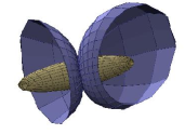
Figure 7. Discrete flat surfaces of revolution and their caustics, shown in the Klein model for $\mathbb{H}^{3}$. The left surface is called a ”snowman”, and the one on the right is called an ”hourglass”.

Example 4.12.

Like in the smooth case (Example 3.9), we can use discrete holomorphic exponential functions $g_{m,n}=e^{c(m+in)}$ for any nonzero constant $c\in\mathbb{R}\cup(i\mathbb{R})$ to construct discrete flat surfaces of revolution. See Figure 7.

Remark 4.13.

In Figure 7, we use the Klein model for $\mathbb{H}^{3}$. We sometimes find the Klein ball model to be more convenient than the Poincare ball model, because geodesics in the Klein model are the same as Euclidean straight lines. Since we are dealing with discrete surfaces with geodesic edges, this can be convenient. This is particularly useful when looking at the intersection set of two discrete surfaces.

5. An example related to the Airy equation, and Stokes phenomenon

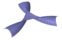
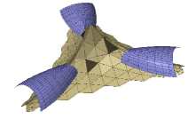
Figure 8. A discrete flat surface in the Klein model constructed from the discrete holomorphic function $z^{4/3}$, and thus related to the Airy equation. The surface is on the left, and the surface together with its discrete caustic is on the right. Because the discrete version of $z^{\gamma}$ is constructed from circle packings, every fourth vertex has two adjacent horizontal (resp. vertical) edges for which $|dg=g_{q}-g_{p}|$ is the same. Since $|dg|$ determines the distance to focal points, we always have three normal geodesics off vertices of the surface meeting at a single focal point. It follows that $C_{f}$ consists of triangles in this case.

The following Example 5.1 is of interest because it has similar properties to the corresponding surface in the smooth case: the surface in the smooth case has trifold symmetry and has three swallowtail singularities connected by three cuspidal edges, and also has a Stokes phenomenon in its asymptotic behavior [28] (see Example 3.10).

5.1. The discrete flat surface made with the discrete power function $z^{4/3}$

We now give an example related to the Airy equation.

Example 5.1.

For this discrete example (see Figure 8), we need the discrete version of $g=z^{4/3}$, as defined in Section 2.2. Because we have a discrete holomorphic function $z^{4/3}$, we are in a position to be able to consider the resulting discrete flat surface via Equations (4.3), (4.7) and (4.8), and also a discrete Airy equation, analogous to Equation (3.5).

Numerical evidence (see Figure 8) suggests similar corresponding swallowtail singularities for this discrete flat surface, analogous to those for the smooth case in Example 3.10.

In Figure 9, portions of the hyperbolic Schwarz image (i.e. this discrete flat surface) related to the Airy equation are shown. The image of the discrete half-line $z>0$ ($z\in\mathbb{Z}$) is drawn in red, which has a single limit point in the boundary sphere. The image of the discrete half-line $iz<0$ ($z\in i\mathbb{Z}$) is drawn in blue, which has no single limit point in the boundary sphere and instead wraps around infinitely many times. This behavior is typical for the continuous Airy case along the Stokes direction, and the corresponding curves on the smooth flat surface associated with the Airy equation behave in the same way (see Example 3.10). This provides a numerical confirmation of a Stokes phenomenon for the discrete Airy function.

We also note that the numerics suggest a behavior similar to that of the smooth case regarding singularities, as the image looks from a distance as though it has three cuspidal edge arcs connecting at three swallowtail singularities. Furthermore the discrete caustic of this flat surface has a similar behavior to that of the corresponding smooth caustic, in that it points sharply outward at its center of symmetry. (Caustics will be introduced in the next section.)

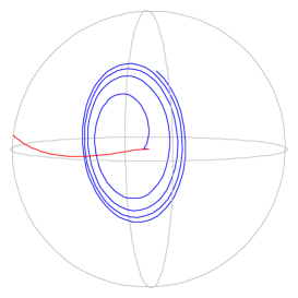
Figure 9. Asymptotic limit of two curves in the discrete flat surface associated with the Airy equation.

$t=0$ (flat)	$t=1/10$
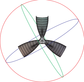
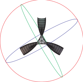
$t=1/2$	$t=1$ (CMC1)

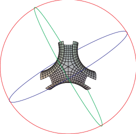
Figure 10. The linear Weingarten family of discrete surfaces for a discrete flat surface associated with the Airy equation, in the Poincare ball model. (The upper-left surface here is the same as the left-hand surface in Figure 8.)

6. Caustics of discrete flat surfaces

In this and the next section (and in Appendix 9), since we will consider flat surfaces and their caustics exclusively, we will abbreviate the notation ”$f_{0}$” to ”$f$”.

6.1. Definition of discrete caustics

Let $C_{f}$ be the collection of focal points, i.e. the focal surface, also called the caustic, of a smooth flat surface $f$ in $\mathbb{H}^{3}$ (note that we should assume $f$ is a flat front, so that the caustic will exist). If $E_{f}$ is the lift of $f=E_{f}\bar{E}_{f}^{T}$ (determined from $g$), then (see [18])

(6.1) $$E_{C_{f}}=E_{f}\cdot\begin{pmatrix}\sqrt{g^{\prime}}&0\\ 0&\frac{1}{\sqrt{g^{\prime}}}\end{pmatrix}\cdot P\;,\;\;\;\;\;P=\frac{1}{\sqrt{2}}\begin{pmatrix}1&\sqrt{-1}\\ \sqrt{-1}&1\end{pmatrix}\;,$$

is a lift of $C_{f}=E_{C_{f}}\bar{E}_{C_{f}}^{T}$. Although we have just described the caustic in terms of Weierstrass data, it is independent of the choice of that data. We know that $C_{f}$ is a flat surface (see [18], [19]), because its lift $E_{C_{f}}$ satisfies the following equation:

(6.2) $$(E_{C_{f}})^{-1}dE_{C_{f}}=\begin{pmatrix}0&1+\frac{\sqrt{-1}}{2}\frac{g^{\prime\prime}}{g^{\prime}}\\ 1-\frac{\sqrt{-1}}{2}\frac{g^{\prime\prime}}{g^{\prime}}&0\end{pmatrix}dz\;.$$

For the case of a discrete flat surface $f$ in $\mathbb{H}^{3}$ with discrete lift $E$, we must first consider how to define the caustic $C_{f}$. We can define the normal $N_{p}$ as in (4.9) at each vertex $f_{p}$ of $f$, so we have normal geodesics emanating from each vertex, and we can consider when normal geodesics of adjacent vertices will intersect. Once we have those intersection points, we will see that we can consider them as vertices of $C_{f}$, giving us a definition for $C_{f}$.

Lemma 6.1.

Let $f$ be a discrete flat surface in $\mathbb{H}^{3}$ with lift $E$, as in (4.10), constructed using the discrete holomorphic function $g$. Let $\alpha_{pq}$ be a cross ratio factorizing function for $g$. Then the normal geodesics in $\mathbb{H}^{3}$ emanating from two adjacent vertices $f_{p}$ and $f_{q}$ will intersect if and only if $\lambda\alpha_{pq}<0$, in which case the intersection point is unique and is equidistant from $f_{p}$ and $f_{q}$. Furthermore, even when the two normal geodesics do not intersect, they still lie in a single common geodesic plane.

Proof.

Consider one edge $pq$. Applying an isometry of $\mathbb{H}^{3}$ if necessary, we may assume without loss of generality that

$$E_{p}=I\;,\;\;f_{p}=\frac{1}{\det E_{p}}E_{p}\bar{E}_{p}^{T}=I\;,\;\;N_{p}=\begin{pmatrix}1&0\\ 0&-1\end{pmatrix}\;.$$

Then, with $dg_{pq}=g_{q}-g_{p}$,

$$E_{q}=\begin{pmatrix}1&dg_{pq}\\ \frac{\lambda\alpha_{pq}}{dg_{pq}}&1\end{pmatrix}\;,\;\;\det E_{q}=1-\lambda\alpha_{pq}\;.$$

Thus

$$f_{q}=\frac{1}{1-\lambda\alpha_{pq}}E_{q}\bar{E}_{q}^{T}\;\;\text{and}\;\;N_{q}=\frac{1}{1-\lambda\alpha_{pq}}E_{q}\begin{pmatrix}1&0\\ 0&-1\end{pmatrix}\bar{E}_{q}^{T}\;.$$

The condition for the two normal geodesics to intersect is that there exist reals $t_{1}$ and $t_{2}$ so that

$$\cosh t_{1}\cdot\begin{pmatrix}1&0\\ 0&1\end{pmatrix}+\sinh t_{1}\cdot\begin{pmatrix}1&0\\ 0&-1\end{pmatrix}=\frac{\cosh t_{2}}{1-\lambda\alpha_{pq}}E_{q}\bar{E}_{q}^{T}+\frac{\sinh t_{2}}{1-\lambda\alpha_{pq}}E_{q}\begin{pmatrix}1&0\\ 0&-1\end{pmatrix}\bar{E}_{q}^{T}\;.$$

In other words (we now abbreviate $dg_{pq}$ to $dg$, and $\alpha_{pq}$ to $\alpha$),

$$(1-\lambda\alpha)\begin{pmatrix}\cosh t_{1}+\sinh t_{1}&0\\ 0&\cosh t_{1}-\sinh t_{1}\end{pmatrix}=\cosh t_{2}\cdot E_{q}\bar{E}_{q}^{T}+\sinh t_{2}\cdot E_{q}\begin{pmatrix}1&0\\ 0&-1\end{pmatrix}\bar{E}_{q}^{T}$$

$$=\cosh t_{2}\cdot\begin{pmatrix}1+|dg|^{2}&\frac{\lambda\alpha}{\overline{dg}}+dg\\ \frac{\lambda\alpha}{dg}+\overline{dg}&1+\frac{\lambda^{2}\alpha^{2}}{|dg|^{2}}\end{pmatrix}+\sinh t_{2}\cdot\begin{pmatrix}1-|dg|^{2}&\frac{\lambda\alpha}{\overline{dg}}-dg\\ \frac{\lambda\alpha}{dg}-\overline{dg}&\frac{\lambda^{2}\alpha^{2}}{|dg|^{2}}-1\end{pmatrix}\;.$$

There exists a $t_{2}$ so that this last sum on the right-hand side is a diagonal matrix if and only if

$$\left|\frac{\lambda\alpha-|dg|^{2}}{\lambda\alpha+|dg|^{2}}\right|>1\;.$$

So the normal lines intersect in $\mathbb{H}^{3}$ if and only if

$$|\lambda\alpha-|dg|^{2}|>|\lambda\alpha+|dg|^{2}|\;.$$

This is equivalent to

$$\lambda\alpha<0\;,$$

and then $t_{2}$ satisfies

$$\sinh(t_{2})=\frac{|dg|^{2}+\lambda\alpha}{\sqrt{-4\lambda\alpha}|dg|}\;,\;\;\;\cosh(t_{2})=\frac{|dg|^{2}-\lambda\alpha}{\sqrt{-4\lambda\alpha}|dg|}\;.$$

Now, to get the diagonal terms in the above matrix equation to match, we want $t_{1}$ such that

$$\cosh(t_{1})=\frac{1}{2(1-\lambda\alpha)}\left[\left(2+|dg|^{2}+\frac{\lambda^{2}\alpha^{2}}{|dg|^{2}}\right)\cosh t_{2}+\left(\frac{\lambda^{2}\alpha^{2}}{|dg|^{2}}-|dg|^{2}\right)\sinh t_{2}\right]\;,$$

$$\sinh(t_{1})=\frac{1}{2(1-\lambda\alpha)}\left[\left(2-|dg|^{2}-\frac{\lambda^{2}\alpha^{2}}{|dg|^{2}}\right)\sinh t_{2}+\left(|dg|^{2}-\frac{\lambda^{2}\alpha^{2}}{|dg|^{2}}\right)\cosh t_{2}\right]\;.$$

Such a $t_{1}$ does exist, and in fact a computation shows that this $t_{1}$ is equal to $t_{2}$.

Now the sign of $t_{2}=t_{1}$ determines which side of the quadrilateral the intersection lies on, and $t_{2}=t_{1}>0$ if and only if $|dg|^{2}+\lambda\alpha>0$.

Note that because $t_{1}=t_{2}$, the distance from the intersection point of the normal lines to either of $f_{p}$ and $f_{q}$ is the same.

By a further isometry of $\mathbb{H}^{3}$ that preserves $f_{p}$ and $N_{p}$, we may change $g$ to $e^{i\theta}g$ for some constant $\theta\in\mathbb{R}$. Thus without loss of generality we may assume $dg_{pq}\in\mathbb{R}$. It is then clear from the above equations that the two geodesics emanating in the normal directions from $f_{p}$ and $f_{q}$ both lie in the geodesic plane $\{x_{2}=0\}\cap\mathbb{H}^{3}$ of $\mathbb{H}^{3}$, with $\mathbb{H}^{3}$ represented as in Section 3.1. This proves the last claim of the lemma. ∎

Remark 6.2.

By an argument similar to that of the proof of Lemma 6.1, but simpler, we also have the following statements: Let $f$ be a discrete flat surface in $\mathbb{H}^{3}$ with lift $E$, as in (4.10), constructed using the discrete holomorphic function $g$. Let $\alpha_{pq}$ be a cross ratio factorizing function for $g$. Let $N_{p}$ denote the normal as in (4.9) at $f_{p}$. Then the lines in $\mathbb{R}^{3,1}$ (not $\mathbb{H}^{3}$) emanating from two adjacent vertices $f_{p}$ and $f_{q}$ in the directions of $N_{p}$ and $N_{q}$ (respectively) will either be parallel or will intersect at a unique point that is equidistant from $f_{p}$ and $f_{q}$. The distance from either $f_{p}$ or $f_{q}$ to that intersection point is

$$\left|\frac{|g_{q}-g_{p}|^{2}+\lambda\alpha_{pq}}{|g_{q}-g_{p}|^{2}-\lambda\alpha_{pq}}\right|\;.$$

This is true on each edge $pq$, regardless of the sign of $\lambda\alpha_{pq}$. Furthermore, these two lines stemming from $f_{p}$ and $f_{q}$ will not be parallel if

$$\lambda\neq\pm\frac{|g_{q}-g_{p}|^{2}}{\alpha_{pq}}\;.$$

Now, for all that follows, we introduce the following assumption.

Assumption: For $g$ the discrete holomorphic map used to construct a discrete flat surface, assume that all quadrilaterals in the image of $g$ in the complex plane are properly embedded.

This implies the following properties:

1. $dg_{pq}$ is never zero for any edge $\overline{pq}$ between adjacent vertices $p$ and $q$ in the domain $D$. Note that this was already assumed in Section 2.3.

2. $dg_{pq}$ and $dg_{ps}$ are never parallel for any square of edge-length $1$ with vertices $p,q,r,s$ in $D$. (If $dg_{pq}$ and $dg_{ps}$ are parallel, then $g_{p},g_{q},g_{r},g_{s}$ all lie in one line, which implies that the interior of the quadrilateral in the complex plane is a half-plane, which is not properly embedded.)

Because the cross ratio for $g$ is always negative, the term $\lambda\alpha_{pq}$ is negative on exactly all of the horizontal edges in the domain $D\subset\mathbb{Z}^{2}$ of $f$, or exactly all of the vertical edges. Applying a $90$ degree rotation to the domain if necessary, we can, and now do, assume without loss of generality that $\lambda\alpha_{pq}$ is negative if and only if the edge $pq$ is vertical in $D$.

Thus every vertical edge $pq$ provides a unique intersection point of the normal geodesics, which we denote by $(C_{f})_{pq}$. The domain $D_{C}$ of this new mesh is now the collection of all vertical edges of $D$. If we let the vertical edges be represented by their midpoints, then we can consider $C_{f}$ to also be defined on a square grid, but now a shifted one, i.e. $D_{C}\subset\mathbb{Z}\times(\mathbb{Z}+\tfrac{1}{2})$.

Definition 6.3.

We call the discrete surface

$$C_{f}=\{(C_{f})_{pq}\,|\,pq\;\text{is a vertical edge}\}$$

the caustic, or focal surface, of $f$.

This new discrete surface $C_{f}$ is generally not a discrete flat surface, as the vertices in the quadrilaterals of the caustic will generally not be concircular. However, it has a number of interesting properties closely related to discrete flat surfaces, which we will describe. The first property is stated in this lemma:

Lemma 6.4.

The quadrilaterals of $(C_{f})_{pq}$ lie in geodesic planes of $\mathbb{H}^{3}$.

Proof.

This is clear from the geometry of the construction, and from the fact that adjacent normal geodesics always lie in a common geodesic plane of $\mathbb{H}^{3}$, by Lemma 6.1. ∎

6.2. Discrete extrinsic curvature: first approach

Now that we have seen the proof of Lemma 6.1, we are able to give one geometric justification for why we can say the discrete surfaces in Section 4.3 are ”flat”. We will give an argument here showing the ”discrete extrinsic curvature” is identically $1$.

For a smooth flat surface given by a frame $E$ solving (3.4), we find that the two functions

$$k_{1}=\frac{-1+|g_{x}|^{2}}{1+|g_{x}|^{2}}\;,\;\;\;k_{2}=\frac{1+|g_{y}|^{2}}{-1+|g_{y}|^{2}}\;$$

give the principal curvatures of the surface, and also give the inverses of the distances to the focal points in $\mathbb{R}^{3,1}$ of the curves in the surface along which either $y$ or $x$ is constant. Here we are considering the focal points found in $\mathbb{R}^{3,1}$ (not $\mathbb{H}^{3}$), but we are finding those focal points with respect to the normal directions to the surface in $\mathbb{H}^{3}$ given by the normal vectors (3.3), which are actually tangent vectors to $\mathbb{H}^{3}$ itself. Since the extrinsic curvature $k_{1}k_{2}$ is exactly $1$, if $k_{1}\neq k_{2}$, we have $|k_{1}|<1$ and $|k_{2}|>1$, and we have that

(6.3) $$\text{arctanh}\left(k_{1}\right)-\text{arctanh}\left(k_{2}^{-1}\right)=\text{arctanh}\left(\frac{-1+|g_{x}|^{2}}{1+|g_{x}|^{2}}\right)-\text{arctanh}\left(\frac{-1+|g_{y}|^{2}}{1+|g_{y}|^{2}}\right)=0\;.$$

This last right-hand equality, of course, is clear from the fact that $|g_{x}|=|g_{y}|$. However, the right-hand equality encodes that the extrinsic curvature is exactly $1$ in a way that can be applied to the discrete case, as follows: the corresponding equation in the discrete case is given by the corresponding summation about the four edges (assume $\lambda\alpha_{pq}=\lambda\alpha_{rs}>0$ and $\lambda\alpha_{qr}=\lambda\alpha_{sp}<0$ – the other case can be handled similarly)

(6.4) $$\text{arctanh}\left(\frac{-\lambda\alpha_{pq}+|g_{q}-g_{p}|^{2}}{\lambda\alpha_{pq}+|g_{q}-g_{p}|^{2}}\right)-\text{arctanh}\left(\frac{\lambda\alpha_{qr}+|g_{r}-g_{q}|^{2}}{-\lambda\alpha_{qr}+|g_{r}-g_{q}|^{2}}\right)+$$

$$\text{arctanh}\left(\frac{-\lambda\alpha_{rs}+|g_{s}-g_{r}|^{2}}{\lambda\alpha_{rs}+|g_{s}-g_{r}|^{2}}\right)-\text{arctanh}\left(\frac{\lambda\alpha_{sp}+|g_{p}-g_{s}|^{2}}{-\lambda\alpha_{sp}+|g_{p}-g_{s}|^{2}}\right)=0$$

of each quadrilateral with vertices associated to $p,q,r,s$ (given in counterclockwise order about the quadrilateral in $D$) in the discrete surface. The analogous geometric meaning of

$$\frac{-\lambda\alpha_{pq}+|g_{q}-g_{p}|^{2}}{\lambda\alpha_{pq}+|g_{q}-g_{p}|^{2}}$$

is preserved in the discrete case, as it is the inverse of the (oriented) distance from either $f_{p}$ or $f_{q}$ to the intersection point of the geodesics in $\mathbb{R}^{3,1}$ stemming off of $f_{p}$ and $f_{q}$ in the directions of $N_{p}$ and $N_{q}$, respectively (see Remark 6.2). Furthermore, Equation (6.4) follows immediately from the definition of the cross ratio factorizing function $\alpha$. In this sense, we can say that the “discrete extrinsic curvature” is identically $1$.

6.3. Discrete extrinsic curvature: second approach

We now consider a second approach to discrete extrinsic curvature. For a smooth surface of constant extrinsic curvature $1$, the infinitesimal ratio of the area of the Gauss map to the area of the surface is exactly $1$. So another way to give a notion that the ”discrete extrinsic curvature” be identically $1$ for a discrete flat surface is to show the analogous property in the discrete case. That is the purpose of the following lemma.

Lemma 6.5.

Let $f$ be a discrete flat surface in $\mathbb{H}^{3}$ with normal map $N$. Consider the vertices $f_{p},f_{q},f_{r},f_{s}$ of one quadrilateral (in $\mathbb{H}^{3}$) of the surface associated with the quadrilateral with vertices $p$, $q$, $r$, $s$ (given in counterclockwise order) in $D$. These four vertices $f_{p},f_{q},f_{r},f_{s}$ also determine another quadrilateral $\mathcal{F}_{f}$, now in $\mathbb{R}^{3,1}$, again with vertices $f_{p},f_{q},f_{r},f_{s}$, but now with geodesic edges $\overline{f_{p}f_{q}}$, $\overline{f_{q}f_{r}}$, $\overline{f_{r}f_{s}}$, $\overline{f_{s}f_{p}}$ in $\mathbb{R}^{3,1}$, and which is planar in $\mathbb{R}^{3,1}$. Likewise, the normals $N_{p},N_{q},N_{r},N_{s}$ determine a planar quadrilateral $\mathcal{F}_{N}$ in $\mathbb{R}^{3,1}$ with vertices $N_{p},N_{q},N_{r},N_{s}$ and with geodesic edges $\overline{N_{p}N_{q}}$, $\overline{N_{q}N_{r}}$, $\overline{N_{r}N_{s}}$, $\overline{N_{s}N_{p}}$ in $\mathbb{R}^{3,1}$.

These two quadrilaterals $\mathcal{F}_{f}$ and $\mathcal{F}_{N}$ lie in parallel spacelike planes of $\mathbb{R}^{3,1}$ and have the same area.

Proof.

Because $f_{p},f_{q},f_{r},f_{s}$ lie in a circle $\mathcal{C}$ in $\mathbb{H}^{3}$, there exists a planar quadrilateral $\mathcal{F}_{f}$ in $\mathbb{R}^{3,1}$ with edges that are geodesics in $\mathbb{R}^{3,1}$, and with vertices $f_{p},f_{q},f_{r},f_{s}$.

Since $N_{p}$ and $N_{q}$ have reflective symmetry with respect to the edge of $\mathcal{F}_{f}$ from $f_{p}$ and $f_{q}$ (see Remark 6.2), and since similar symmetry holds on the other three edges of $\mathcal{F}_{f}$, we know that $f_{p}+N_{p},f_{q}+N_{q},f_{r}+N_{r},f_{s}+N_{s}$ are the vertices of a planar quadrilateral $\mathcal{F}_{f+N}$ with geodesic edges in $\mathbb{R}^{3,1}$. It follows that $N_{p},N_{q},N_{r},N_{s}$ are then the vertices of a planar quadrilateral $\mathcal{F}_{N}$ with geodesic edges in $\mathbb{R}^{3,1}$. In fact, $\mathcal{F}_{f}$, $\mathcal{F}_{f+N}$ and $\mathcal{F}_{N}$ all lie in parallel spacelike planes.

The goal is to show that $\mathcal{F}_{f}$ and $\mathcal{F}_{N}$ have the same area. Since $\mathcal{F}_{f}$ and $\mathcal{F}_{N}$ are parallel, it is allowable to replace the metric of $\mathbb{R}^{3,1}$ with the standard positive-definite Euclidean metric for $\mathbb{R}^{4}$ and simply prove that $\mathcal{F}_{f}$ and $\mathcal{F}_{N}$ have the same area with respect to that metric. The advantage of this is that it allows us to use known computational methods involving mixed areas. See [10], for example, for an explanation of mixed areas.

Noting that $f\pm N$ lies in the $3$-dimensional light cone of $\mathbb{R}^{3,1}$, i.e. $\langle f+N,f+N\rangle=\langle f-N,f-N\rangle=0$, we define the lightlike vectors

$$G_{1}=\tfrac{1}{2}(f+N)\;,\;\;\;G_{2}=\tfrac{1}{2}(f-N)\;.$$

(In fact, the normal geodesic at each vertex of $f$ in $\mathbb{H}^{3}$ is asymptotic to the lines in the light cone determined by $G_{1}$ and $G_{2}$.) The two concircular sets $\{(G_{1})_{p},(G_{1})_{q},(G_{1})_{r},(G_{1})_{s}\}$ and $\{(G_{2})_{p},(G_{2})_{q},(G_{2})_{r},(G_{2})_{s}\}$ have the same real cross ratio, so the two quadrilaterals in $\mathbb{R}^{3,1}$ that they determine are either congruent or dual to each other. In fact, they are dual to each other, seen by examining the four distances to intersection points amongst the normal lines in $\mathbb{R}^{3,1}$ extending from $f_{p}$, $f_{q}$, $f_{r}$ and $f_{s}$ (two of which to one side of $\mathcal{F}_{f}$ are less than $1$, and the other two of which to the opposite side are greater than $1$, see the proof of Lemma 6.1 and also Remark 6.2). It follows that the mixed area of $G_{1}$ and $G_{2}$ is zero [10]. We then have, with “$A$” denoting area and “$MA$” denoting mixed area,

$$A(f)=A(G_{1}+G_{2})=A(G_{1})+A(G_{2})+2MA(G_{1},G_{2})=A(G_{1})+A(G_{2})\;,$$

$$A(N)=A(G_{1}-G_{2})=A(G_{1})+A(G_{2})-2MA(G_{1},G_{2})=A(G_{1})+A(G_{2})\;.$$

Hence $A(f)=A(N)$. ∎

Remark 6.6.

The proof of Lemma 6.1 shows that for a vertical edge $\overline{pq}$ (of length $1$) of $D$, the geodesic edge $\overline{f_{p}f_{q}}$, the geodesic through $f_{p}$ in the direction of $N_{p}$ and the geodesic through $f_{q}$ in the direction of $N_{q}$ form the boundary of a planar equilateral triangle in $\mathbb{H}^{3}$. In particular, it follows that $f_{p}$, $f_{q}$, $f_{q}^{d}$ and $f_{p}^{d}$ are concircular, for any value of $d$. One can also show that $f_{p}$, $f_{q}$, $f_{q}^{d}$ and $f_{p}^{d}$ are concircular even when $\overline{pq}$ is a horizontal edge in $D$. This shows that the quadrilaterals formed by the two points of an edge and the two points of the corresponding edge of a parallel flat surface are always concircular. This in turn implies that a quadrilateral of the surface and the corresponding quadrilateral on a parallel surface have a total of eight vertices all lying on a common sphere - forming a cubical object with concircular sides. This gives (see [5]) a discrete version of a triply orthogonal system, that is, a map from $\mathbb{Z}^{3}$ or a subdomain of $\mathbb{Z}^{3}$ to $\mathbb{R}^{3}$ where all quadrilaterals are concircular.

6.4. A formula for the caustic

In Lemma 6.4 we gave one property of caustics that is closely related to discrete flat surfaces. Here we give a second such type of property, as seen in Theorem 6.7 below.

The equation for the lift $E$ of $f$ is

$$E_{p}^{-1}E_{q}=\begin{pmatrix}1&dg_{pq}\\ \frac{\lambda\alpha_{pq}}{dg_{pq}}&1\end{pmatrix}\;.$$

However, since the formula (4.8) for the surface has a mitigating scalar factor $1/\det E$, we can change the equation above so that the potential matrix has determinant one, without changing the resulting surface, so let us instead use:

$$\tilde{E}_{p}=\frac{1}{\sqrt{\det E_{p}}}E_{p}\;,\;\;\;f_{p}=\tilde{E}_{p}\overline{\tilde{E}_{p}}^{T}\;,$$

$$\tilde{E}_{p}^{-1}\tilde{E}_{q}=\frac{1}{\sqrt{1-\lambda\alpha_{pq}}}\begin{pmatrix}1&dg_{pq}\\ \frac{\lambda\alpha_{pq}}{dg_{pq}}&1\end{pmatrix}\;.$$

We also now assume that $\lambda$ is sufficiently close to zero so that

$$|\lambda\alpha_{pq}|<1$$

for all edges $pq$.

We now define, for each vertical edge $pq$,

(6.5) $$E_{(C_{f})_{pq}}=(a\tilde{E}_{p}+b\tilde{E}_{q})\cdot\begin{pmatrix}\frac{\sqrt{dg_{pq}}}{\sqrt[4]{\lambda\alpha_{pq}}}&0\\ 0&\frac{\sqrt[4]{\lambda\alpha_{pq}}}{\sqrt{dg_{pq}}}\end{pmatrix}\cdot P\;,$$

where $a$ and $b$ are any choice of nonnegative reals such that $a+b=1$ (recall the definition of $P$ in (6.1)). This is a natural discretization of the $E_{C_{f}}$ for the case of smooth surfaces (see (6.1)), where we now must take a weighted average of $E_{p}$ and $E_{q}$, and we allow any choice of weighting $(a,b)$. For the smooth case in Equation (3.4), the fourth root of the upper right term of $E^{-1}dE$ divided by the lower left term gives the $\sqrt{g^{\prime}}$ appearing in Equation (6.1). For the discrete case in Equation (4.10), the fourth root of the upper right term of $E_{p}^{-1}(E_{q}-E_{p})$ divided by the lower left term gives the $\sqrt{dg_{pq}}/\sqrt[4]{\lambda\alpha_{pq}}$ appearing in Equation (6.5) here. This explains why we insert the $\sqrt[4]{\lambda\alpha_{pq}}$ factors here. Note that $\sqrt[4]{\lambda\alpha_{pq}}$ is not real, because $\lambda\alpha_{pq}<0$.

Theorem 6.7.

The formula

(6.6) $$C_{f}=\frac{1}{\det(E_{C_{f}})}E_{C_{f}}\cdot\overline{E_{C_{f}}}^{T}$$

for the discrete caustic holds for all vertical edges $pq$, and this formula does not depend on the choice of $a$ and $b=1-a$.

Proof.

A computation gives

$$(E_{C_{f}})_{pq}\overline{(E_{C_{f}})_{pq}}^{T}=S\cdot\tilde{E}_{p}\begin{pmatrix}\frac{|dg_{pq}|}{\sqrt{-\lambda\alpha_{pq}}}&0\\ 0&\frac{\sqrt{-\lambda\alpha_{pq}}}{|dg_{pq}|}\end{pmatrix}\bar{\tilde{E}}_{p}^{T}=\frac{S}{\det E_{p}}\cdot E_{p}\begin{pmatrix}\frac{|dg_{pq}|}{\sqrt{-\lambda\alpha_{pq}}}&0\\ 0&\frac{\sqrt{-\lambda\alpha_{pq}}}{|dg_{pq}|}\end{pmatrix}\bar{E}_{p}^{T}\;,$$

$$S=1+2ab\frac{1-\sqrt{1-\lambda\alpha_{pq}}}{\sqrt{1-\lambda\alpha_{pq}}}\;.$$

The scalar factor $S$ is the only part of $(E_{C_{f}})_{pq}\overline{(E_{C_{f}})_{pq}}^{T}$ that depends on $a$ and $b$, but this scalar factor is irrelevant in the formula (6.6), so we see independence from the choice of $a$ and $b$. The result now follows from the proof of Lemma 6.1. ∎

Remark 6.8.

However, the choice of normal direction at the vertices of $C_{f}$ does depend on the choice of $a$ and $b$, as the following equation shows:

(6.7) $$N_{pq}=(\tilde{E}_{C_{f}})_{pq}\begin{pmatrix}1&0\\ 0&-1\end{pmatrix}\overline{(\tilde{E}_{C_{f}})_{pq}}^{T}=\tilde{E}_{p}\Omega\bar{\tilde{E}}_{p}^{T}\;,$$

where $\Omega$ is

$$\begin{pmatrix}\frac{2b}{\sqrt{1-\lambda\alpha_{pq}}}(a+\frac{b}{\sqrt{1-\lambda\alpha_{pq}}})|dg_{pq}|&\left(\left(a+\frac{b}{\sqrt{1-\lambda\alpha_{pq}}}\right)^{2}+\frac{b^{2}}{1-\lambda\alpha_{pq}}\lambda\alpha_{pq}\right)\frac{\sqrt{dg_{pq}}}{\overline{\sqrt{dg_{pq}}}}\\ \left(\left(a+\frac{b}{\sqrt{1-\lambda\alpha_{pq}}}\right)^{2}+\frac{b^{2}}{1-\lambda\alpha_{pq}}\lambda\alpha_{pq}\right)\frac{\overline{\sqrt{dg_{pq}}}}{\sqrt{dg_{pq}}}&\frac{2b}{\sqrt{1-\lambda\alpha_{pq}}}(a+\frac{b}{\sqrt{1-\lambda\alpha_{pq}}})\frac{\lambda\alpha_{pq}}{|dg_{pq}|}\end{pmatrix}\;.$$

Equation (6.7) implies that, for both horizontal and vertical edges, the adjacent normal geodesics of the caustic typically do not intersect, for any generic choice of $a$ and $b$.

7. Singularities of discrete flat surfaces

The purpose of the next results is to show that the discrete caustics in Section 6 have properties similar to the caustics in the smooth case.

In what follows, we will regard both the discrete flat surface $f$ and its caustic $C_{f}$ as discrete surfaces that have edges and faces in $\mathbb{H}^{3}$ (not just vertices). Since there is a unique geodesic line segment between any two points in $\mathbb{H}^{3}$, the edge between any two adjacent vertices of $f$ is uniquely determined. The same is true of $C_{f}$. Then, since the image of the four vertices of any given fundamental quadrilateral in $D$ (resp. in $D_{C}$) under $f$ (resp. $C_{f}$) has image lying in a single geodesic plane (see Theorem 4.6 and Lemma 6.4), the image of the fundamental quadrilateral in $D$ (resp. $D_{C}$) can be regarded as a quadrilateral in a geodesic plane of $\mathbb{H}^{3}$ bounded by four edges of $f$ (resp. $C_{f}$). This is the setting for the results given in this section.

In the case of a smooth flat surface (front) $f$ in $\mathbb{H}^{3}$ and its smooth flat caustic $C_{f}$, every point in $C_{f}$ is a point in the singular set of one of the parallel flat surfaces of $f$. In Lemma 7.1, we are stating that every point in the discrete caustic $C_{f}$ of a discrete flat surface $f$ is a point in the edge set of some parallel flat surface of $f$. This, in conjuction with Theorem 7.3, suggests a natural candidate for the definition of the singular set of a discrete flat surface. The proof of Lemma 7.1 is immediate from the definitions of parallel surfaces and caustics.

Lemma 7.1.

Let $f$ be a discrete flat surface defined on a domain $D\subseteq\mathbb{Z}^{2}$ determined by a discrete holomorphic function $g:D\to\mathbb{C}$ with properly embedded quadrilaterals, and let $C_{f}$ be its caustic. Let $P\in\mathbb{H}^{3}$ be any point in $C_{f}$, so $P$ lies in the quadrilateral $\mathcal{F}$ of $C_{f}$ that is determined by two adjacent vertices $f_{p}$, $f_{q}$ of $f$ and the normal geodesics (which contain two opposite edges of $\mathcal{F}$) in the directions $N_{p}$, $N_{q}$ at $f_{p}$, $f_{q}$, respectively. (Thus $\overline{pq}$ will be a horizontal edge of $D$.) $P$ can lie in either the interior of $\mathcal{F}$, or an edge of $\mathcal{F}$, or could be a vertex of $\mathcal{F}$.

Then $P$ lies in the edge $\overline{f_{p}^{d}f_{q}^{d}}$ of some parallel surface $f^{d}$ of $f$.

The next proposition will be used in the proof of Theorem 7.3.

Proposition 7.2.

Let $f$ be a discrete flat surface with normal $N$ produced from a discrete holomorphic function $g$ with properly embedded quadrilaterals. Then for all vertices $p$, $N_{p}$ is not tangent to any quadrilateral of $f$ having vertex $f_{p}$.

Proof.

Take a quadrilateral with vertices $f_{p}$, $f_{q}$, $f_{r}$ and $f_{s}$ of $f$ so that $\overline{pq}$ is a horizontal edge of $D$. We may make all of the assumptions in the proof of Lemma 6.1, including the assumption that $dg_{pq}$ is real. Of course, the normal $N_{p}=\text{diag}(1,-1)$ lies in the hyperplane $\{x_{2}=0\}$ of $\mathbb{R}^{3,1}$ (here we regard points of $\mathbb{R}^{3,1}$ as Hermitean matrices as in Section 3.1), and so does the point $f_{q}$, since $dg_{pq}\in\mathbb{R}$. Furthermore, $\overline{pq}$ is a horizontal edge of $D$, so $\lambda\alpha_{pq}>0$, which implies that $f_{q}$ does not lie in the geodesic in $\mathbb{H}^{3}$ containing $f_{p}$ and tangent to $N_{p}$. However, $g$ has properly embedded quadrilaterals, so both $dg_{ps}$ and $\tfrac{\lambda\alpha_{ps}}{dg_{ps}}+\overline{dg_{ps}}$ will not lie in $\mathbb{R}$, and thus $f_{s}$ will not lie in the hyperplane $\{x_{2}=0\}$. It follows that $N_{p}$ will not be parallel to the geodesic plane in $\mathbb{H}^{3}$ containing the two geodesics from $f_{p}$ to $f_{q}$ and from $f_{p}$ to $f_{s}$. ∎

For a smooth flat surface (front) $f$ and its caustic $C_{f}$, a parallel flat surface to $f$, including $f$ itself, will meet $C_{f}$ along its singular set, and that singular set is generally a graph in the combinatorial sense (whose edges consist of immersable curves). Furthermore, all vertices of that combinatorial graph have valence at least two. For example, cuspidal edges form the edges of this graph, and swallowtails give vertices of this graph with valence two. In particular, no cuspidal edge can simply stop at some point without continuing on to at least one other cuspidal edge (as this would give a vertex of valence one). The following theorem shows that an analogous property holds in the discrete case. Note that when we are speaking of the vertices of this combinatorial graph in the theorem below, these vertices are not the same as the vertices of the discrete flat surface, nor its discrete caustic, in general.

Theorem 7.3.

Let $f$ be a discrete flat surface defined on a domain $D\subseteq\mathbb{Z}^{2}$ determined by a discrete holomorphic function $g:D\to\mathbb{C}$ with properly embedded quadrilaterals, and let $C_{f}$ be its caustic. Let $f^{d}$ be a parallel surface, and let $S_{d}$ be the set of all $P\in\mathbb{H}^{3}$ as in Lemma 7.1, for that value of $d$, and for any adjacent endpoints $p$ and $q$ of a horizontal edge of $D$. Assume that no two adjacent vertices of $f^{d}$ are ever equal, and that the faces of $C_{f}$ are embedded.

Then $S_{d}$ is a graph (in the combinatorial sense) with edges composed of geodesic segments lying in the image in $\mathbb{H}^{3}$ of the horizontal edges of $D$ under $f^{d}$, and with all vertices of $S_{d}$ having valence at least two.

Remark 7.4.

The snowman shown on the right-hand side of Figure 7 (see Example 4.12) provides an example to which Theorem 7.3 applies. The Airy example in Section 5 also satisfies the conclusion of this theorem (see Figure 8), although it does not actually satisfy the condition in the theorem that the faces of the caustic be embedded.

Remark 7.5.

At least one of the assumptions in Theorem 7.3 that the quadrilaterals of $C_{f}$ are embedded and that no two adjacent vertices of $f^{d}$ coincide is necessary. Without them, the discrete hourglass, as seen in Figure 7 (see Example 4.12), would provide a counterexample to the result. However, it is still an open question whether both of those conditions are really needed. There are reasons why it is not obvious that we can remove one of those two conditions. We explore those reasons in Appendix 9.

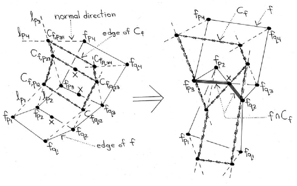
Figure 11. A graphical representation of the argument in the proof of Theorem 7.3.

Proof.

We must show that all vertices of $S_{d}$ have valence at least two. There are essentially only two situations for which we need to show this, one obvious and one not obvious. The obvious case is when an entire edge $\overline{f_{p}^{d}f_{q}^{d}}$ lies in $S_{d}$, and then the result is clear. The non-obvious case that we now describe, where only a part of $\overline{f_{p}^{d}f_{q}^{d}}$ lies in $S_{d}$, is essentially only one situtation, since any other non-obvious situation can be reformulated in terms of the notation given below. Without loss of generality, replacing $f^{d}$ by $f$ if necessary, we may assume that $d=1$.

Let $D$ be a domain in $\mathbb{Z}^{2}$ containing $p_{1}=(0,1)$, $p_{2}=(0,2)$, $p_{3}=(0,3)$, $p_{4}=(0,4)$, $q_{1}=(1,1)$, $q_{2}=(1,2)$, $q_{3}=(1,3)$, $q_{4}=(1,4)$, and let $g$ be a discrete holomorphic function defined on $D$. Let $f=f^{1}$ be the resulting discrete flat surface. We have a normal direction defined at each vertex of $f$, which determines normal geodesics $\ell_{p_{i}}$, $\ell_{q_{i}}$ at the vertices $f_{p_{i}}$, $f_{q_{i}}$, respectively. Note that $\ell_{p_{i}}$ and $\ell_{q_{i}}$ never intersect (and thus $f_{p_{i}}$ and $f_{q_{i}}$ are never equal), although they do lie in the same geodesic plane, and that $\ell_{p_{i}}$ and $\ell_{p_{i+1}}$ (resp. $\ell_{q_{i}}$ and $\ell_{q_{i+1}}$) intersect at a single point that we call $C_{f,p_{i,i+1}}$ (resp. $C_{f,q_{i,i+1}}$), by Lemma 6.1. The point $C_{f,p_{i,i+1}}$ (resp. $C_{f,q_{i,i+1}}$) is equidistant from the two vertices $f_{p_{i}}$ and $f_{p_{i+1}}$ (resp. $f_{q_{i}}$ and $f_{q_{i+1}}$), as in Lemma 6.1.

Now the caustic $C_{f}$ has two quadrilaterals, described here by listing their vertices in order about each quadrilateral:

$$\mathcal{F}_{1}=(C_{f,p_{12}},C_{f,q_{12}},C_{f,q_{23}},C_{f,p_{23}})\;\;\;\text{and}\;\;\;\mathcal{F}_{2}=(C_{f,p_{23}},C_{f,q_{23}},C_{f,q_{34}},C_{f,p_{34}})\;.$$

Let $x$ be a point in the geodesic edge $\overline{f_{p_{2}}f_{q_{2}}}$ so that $x$ also lies in the edge $\overline{C_{f,p_{23}}C_{f,q_{23}}}$. Since no two adjacent vertices of $f$ are ever equal, it follows that $x$ lies strictly in the interior of $\overline{f_{p_{2}}f_{q_{2}}}$. (See the left-hand side of Figure 11.) Thus, since the face $\mathcal{F}_{1}$ of the caustic is embedded, there exists a half-open interval $\mathcal{I}=(y,x]$ or $\mathcal{I}=[x,y)$ contained entirely in the interior of $\overline{f_{p_{2}}f_{q_{2}}}$ so that $\mathcal{I}$ lies in $\mathcal{F}_{1}$.

Thus $x$ can become a vertex of the graph $S_{d=1}$. We wish to show that the valence at $x$ is at least two. This would mean that the visual representation is more like in the right-hand side of Figure 11, where the quadrilateral of $f$ with vertices $f_{p_{2}},f_{q_{2}},f_{q_{3}},f_{p_{3}}$ is nonembedded. It suffices to show that there exists a half-open interval $\tilde{\mathcal{I}}=(\tilde{y},\tilde{x}]$ or $\tilde{\mathcal{I}}=[\tilde{x},\tilde{y})$ contained entirely in the interior of the geodesic edge $\overline{f_{p_{3}}f_{q_{3}}}$ so that:

1. $\tilde{\mathcal{I}}$ lies in the face $\mathcal{F}_{2}$ of the caustic, and

2. $\tilde{x}=x$.

Because $x$ lies in both the geodesic plane determined by $f_{p_{2}},f_{q_{2}},f_{q_{3}},f_{p_{3}}$ and the geodesic plane determined by $f_{p_{3}},f_{q_{3}},C_{f,{q_{23}}},C_{f,{p_{23}}}$, and because Proposition 7.2 implies these two geodesic planes are not equal, $x$ must also lie in the line determined by $\overline{f_{p_{3}},f_{q_{3}}}$. Then, because $x$ lies in the embedded face $\mathcal{F}_{1}$, and because both $\overline{C_{f,p_{23}}C_{f,q_{23}}}$ and $\overline{f_{p_{3}}f_{q_{3}}}$ lie in the geodesic planar region between $\ell_{p_{3}}$ and $\ell_{q_{3}}$, $x$ must lie in the edge $\overline{f_{p_{3}},f_{q_{3}}}$ itself. (Note that we have now proven that the quadrilateral with vertices $f_{p_{2}}$, $f_{q_{2}}$, $f_{q_{3}}$ and $f_{p_{3}}$ is not embedded, so in fact the visual representation must be more like in the right-hand side of Figure 11.)

Keeping in mind that $x$ also lies in the edge $\overline{C_{f,p_{23}},C_{f,q_{23}}}$, then since both edges $\overline{f_{p_{3}},f_{q_{3}}}$ and $\overline{C_{f,p_{23}},C_{f,q_{23}}}$ lie in the plane determined by $\mathcal{F}_{2}$, and since $\mathcal{F}_{2}$ is embedded, we conclude existence of such an interval $\tilde{\mathcal{I}}$ with the required properties. ∎

The above Lemma 7.1 and Theorem 7.3 suggest that $S_{d}$ has many of the right properties to make it a natural candidate for the singular set of any discrete surface $f^{d}$ in the parallel family of $f$.

Remark 7.6.

We have chosen to consider the set $S_{d}$ in the image $f(D)$ of a discrete flat surface, rather than in the domain $D$ itself (as is usually done for the singular set in the smooth case), because $S_{d}$ becomes a collection of connected curves in the image, while in the domain $D$ it would jump discontinuously between points in the lower and upper horizontal edges of quadrilaterals of $D$ (as we have seen in the above proof). However, one could remedy this by inserting vertical lines between those lower and upper edge points in quadrilaterals of $D$, and then consider the set in the domain.

8. Appendix: the discrete power function

In Figure 10, we have drawn some of the discrete surfaces in the linear Weingarten family associated with the discretization of the Airy equation. For constructing these graphics, we used the discrete holomorphic power function. We explain here how to solve the difference equation for determining the discrete power function, as follows:

$$\text{cr}_{m,n}=\frac{(g_{m,n}-g_{m+1,n})(g_{m+1,n+1}-g_{m,n+1})}{(g_{m+1,n}-g_{m+1,n+1})(g_{m,n+1}-g_{m,n})}=-1\;,$$

$$\gamma g_{m,n}=2m\frac{(g_{m+1,n}-g_{m,n})(g_{m,n}-g_{m-1,n})}{g_{m+1,n}-g_{m-1,n}}+2n\frac{(g_{m,n+1}-g_{m,n})(g_{m,n}-g_{m,n-1})}{g_{m,n+1}-g_{m,n-1}}\;,$$

with the initial conditions

$$g_{0,0}=0,\quad g_{1,0}=1,\quad g_{0,1}=i^{\gamma}\;.$$

Once we know $g_{m,0}$ and $g_{0,n}$, the full solution is given by solving the first equation for the cross ratio.

We fix $n$ and set

$$g_{m}=g_{m,n}\quad\hbox{\rm and}\quad G_{m}=g_{m,n+1}\;.$$

Then, it is seen from the cross ratio condition that

$$G_{m+1}-g_{m+1}={(g_{m+1}-g_{m})(G_{m}-g_{m})-(g_{m+1}-g_{m})^{2}\over(g_{m+1}-g_{m})+(G_{m}-g_{m})}\;.$$

If we set

$$a_{m}=G_{m}-g_{m}\quad\hbox{\rm and}\quad p_{m}=g_{m+1}-g_{m}\;,$$

then $\{a_{m}\}$ satisfies

$$a_{m+1}={p_{m}a_{m}-p_{m}^{2}\over a_{m}+p_{m}}\;.$$

We define the recurrence relations:

$$b_{m+1} = p_{m}b_{m}-p_{m}^{2}c_{m},$$

$$c_{m+1} = b_{m}+p_{m}c_{m}$$

so that

$$a_{m}={b_{m}\over c_{m}}\;.$$

The initial conditions are

$$c_{0}=1\quad\hbox{\rm and}\quad b_{0}=g_{0,n+1}-g_{0,n}\;.$$

The relation is written in the form

$$\left(\begin{array}[]{c}b_{m+1}\\ c_{m+1}\end{array}\right)=\left(\begin{array}[]{cc}p_{m}&-p_{m}^{2}\\ 1&p_{m}\end{array}\right)\left(\begin{array}[]{c}b_{m}\\ c_{m}\end{array}\right)$$

and the eigenvalues of the $2\times 2$ matrix just above are $(1\pm i)p_{m}$.

The difference equation satisfied by $c_{m}$ is

$$c_{m+2}-(p_{m}+p_{m+1})c_{m+1}+2p_{m}^{2}c_{m}=0\qquad(c\geq 0)$$

where $c_{0}=1$ and $c_{1}=g_{0,n+1}+g_{1,n}-2g_{0,n}$. Once we have determined $\{c_{m}\}$, then

$$b_{m}=c_{m+1}-p_{m}c_{m}\;\;\;\text{and}\;\;\;a_{m}={b_{m}\over c_{m}}$$

determine

$$G_{m}=g_{m,n}+a_{m}\;.$$

Then, using Equation (2.4), we can determine $g_{m,n}$ for all nonegative $m$ and $n$.

We have the following fact, which was also stated in [3]:

Lemma 8.1.

Suppose that $g_{m,n}$ is the discrete holomorphic function solving (2.3) and (2.4) for one choice of $\gamma$, and suppose $\hat{g}_{m,n}$ is the same, but with $\gamma$ replaced by $\hat{\gamma}=2-\gamma$. Then $g_{m,n}$ and $-\hat{g}_{m,n}$ satisfy Equation (4.13) with $\alpha_{pq}=1$ (resp. $\alpha_{pq}=-1$) on horizontal (resp. vertical) edges.

Proof.

That (4.13) holds on the edges $(m,0)(m+1,0)$ and $(0,n)(0,n+1)$ can be easily confirmed from Equation (2.4). Then an induction argument proves the result on all other edges as well. ∎

Recently, [2] solved this system explicitly in terms of hypergeometric functions.

9. Appendix: On a maximum principle for discrete holomorphic functions

If $g(z)$ is a smooth nonconstant holomorphic function with respect to the usual complex coordinate $z$ for $\mathbb{C}$, then $\log|g|$ is a harmonic function, and the maximum principle for harmonic functions tells us that $\log|g|$ cannot have a local finite minimum at an interior point of the domain. Thus, if $|g|$ has a local minimum at an interior point $z_{0}$, it must be that $g(z_{0})=0$.

There are various ways to discretize the notions of holomorphicity and harmonicity. See [4], [6], [9], [10], [23], [24], [25], [33], to name just a few of the possible references – however, the history of this topic goes back much further than just the references mentioned here. These ways do provide for discrete versions of the maximum principle. The definition we have chosen here for discrete holomorphic functions based on cross ratios, however, does not satisfy a particular simple-minded discrete version of the maximum principle, as we can see by the first explicit example below. A more sophisticated consideration is needed to produce a proper discrete version of the maximum principle, but we do not discuss that here, as the simplest questions are what are relevant to Theorem 7.3.

Example 9.1.

Set $D=\{(m,n)\,|\,-1\leq m\leq 1,-1\leq n\leq 2\}$. Then, with $i=\sqrt{-1}$, set

$$g_{0,-1}=\tfrac{1}{3}-6i\;,\;\;\;g_{0,0}=\tfrac{1}{3}\;,\;\;\;g_{0,1}=\tfrac{1}{3}+i\;,\;\;\;g_{0,2}=\tfrac{10}{3}+10i\;,$$

$$g_{-1,0}=\tfrac{1}{3}-\tfrac{1}{2}\sqrt{35}+\tfrac{1}{2}i+3\cos(-\tfrac{2}{5}\pi)+3i\sin(-\tfrac{2}{5}\pi)\;,$$

$$g_{1,0}=\tfrac{1}{3}+\tfrac{1}{2}\sqrt{15}+\tfrac{1}{2}i+2\cos(-\tfrac{2}{5}\pi)+2i\sin(-\tfrac{2}{5}\pi)\;,$$

and extend $g$ to all of $D$ so that all cross ratios of $g$ on $D$ are $-1$. That is, take $g$ so that all $\alpha_{(m,n)(m+1,n)}=-1$ and all $\alpha_{(m,n)(m,n+1)}=1$. Then we have the following two properties:

1. Amongst all vertices of $D$, $|g|$ has a strict minimum of $1/3$ at the interior vertex $(0,0)$.

2. Amongst all edges of $D$ between adjacent vertices $p$ and $q$ (both horizontal and vertical), $|g_{q}-g_{p}|$ has a strict minimum of $1$ at the interior edge from $(0,0)$ to $(0,1)$.

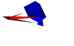
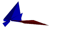
Figure 12. Caustics $C_{f}$ which meet $f^{d}$ for some $d$ at a single point, with $g$ taken as in Examples 9.1 and 9.2. The caustics are shown in red, and the $f^{d}$ are shown in blue.

Taking $g$ as in the previous example, and taking $\lambda=1/100$, we can produce the flat surfaces $f^{d}$ and the caustic $C_{f}$. It turns out that the surface $f^{d}$ and the caustic $C_{f}$ intersect at just one point if $d\approx 1/10$ is chosen correctly. See the left-hand side of Figure 12. In this case, two adjacent vertices (coming from $(0,0)$ and $(0,1)$) of $f^{d}$ do coincide. However, the quadrilaterals of the caustic $C_{f}$ are not embedded in this case, so this example does not suffice to show that both assumptions at the end of the first paragraph of Theorem 7.3 are truly needed.

In light of the equations in the proof of Lemma 6.1, a natural next step toward understanding the role of coincidence of vertices of $f^{d}$ in Theorem 7.3 (and thus toward understanding which assumptions the theorem really needs) is to consider a discrete holomorphic function with the properties as in the next explicit example.

Example 9.2.

Taking the same domain $D$ as in the previous example, we now set

$$g_{0,-1}=1-\tfrac{3}{5}i\;,\;\;\;g_{0,0}=0\;,\;\;\;g_{0,1}=i\;,\;\;\;g_{0,2}=1+\tfrac{8}{5}i\;,$$

$$g_{-1,0}=-\sqrt{90}+\tfrac{1}{2}i+\tfrac{19}{2}\cos(-\tfrac{1}{10}\pi)+\tfrac{19}{2}i\sin(-\tfrac{1}{10}\pi)\;,$$

$$g_{1,0}=-\sqrt{6}+\tfrac{1}{2}i+\tfrac{5}{2}\cos(-\tfrac{3}{5}\pi)+\tfrac{5}{2}i\sin(-\tfrac{3}{5}\pi)\;,$$

and, like in the previous example, we extend $g$ to all of $D$ so that all $\alpha_{(m,n)(m+1,n)}=-1$ and all $\alpha_{(m,n)(m,n+1)}=1$. Then we have the following two properties:

1. Amongst all vertical edges of $D$ between adjacent vertices $p$ and $q$, $|g_{q}-g_{p}|$ has a strict minimum of $1$ at the interior edge from $(0,0)$ to $(0,1)$.

2. Amongst any three vertical edges $pq=(-1,n)(-1,n+1)$ and $pq=(0,n)(0,n+1)$ and $pq=(1,n)(1,n+1)$ at the same height in $D$, $|g_{q}-g_{p}|$ is (strictly) minimized at the central edge $(0,n)(0,n+1)$.

Using the function $g$ in Example 9.2, one might hope that the resulting surface $f^{d}$ would show the necessity of the assumption in Theorem 7.3 that the adjacent vertices of $f^{d}$ do not coincide. However, it turns out that the quadrilaterals of $C_{f}$ are not embedded in this case as well. See the right-hand side of Figure 12, where again $\lambda=1/100$ and $d$ ($\approx 1/10$) is taken so that the two vertices of $f^{d}$ coming from $(0,0)$ and $(0,1)$ coincide.

Because of these subtleties, we leave open the question of whether just one of the two conditions in Theorem 7.3 that

1. the adjacent vertices of $f^{d}$ never coincide, and

2. the caustic has embedded faces

would suffice.

References

- [1] S. I. Agafonov, Discrete Riccati equation, hypergeometric functions and circle patterns of Schramm type, Glasgow Math. J. 47A (2005), 1-16.
- [2] H. Ando, M. Hay, K. Kajiwara and T. Masuda, An explicit formula for the discrete power function associated with circle patterns of Schramm type, preprint 2010.
- [3] A. I. Bobenko, Discrete conformal maps and surfaces, Symmetry and integrability of difference equations, Cambridge Univ. Press, London Math. Soc. Lect. Note Series 255 (1999), 97-108.
- [4] A. I. Bobenko, T. Hoffmann and B. A. Springborn, Minimal surfaces from circle patterns: geometry from combinatorics, Ann. of Math. 164 (2006), 231-264.
- [5] A. I. Bobenko, D. Matthes and Y. B. Suris, Discrete and smooth orthogonal systems: -approximation, Internat. Math. Research Notices 45 (2003), 2415-2459.
- [6] A. I. Bobenko, C. Mercat and Y. B. Suris, Linear and nonlinear theories of discrete analytic functions. Integrable structure and isomonodromic Green’s function, J. Reine und Angew. Math. 583 (2005), 117-161.
- [7] A. I. Bobenko and U. Pinkall, Discrete isothermic surfaces, J. reine angew Math. 475 (1996), 187-208.
- [8] A. I. Bobenko and U. Pinkall, Discretization of surfaces and integrable systems, Oxford Lecture Ser. Math. Appl. 16, Oxford Univ. Press (1999), 3-58.
- [9] A. I. Bobenko and B. A. Springborn, A discrete Laplace-Beltrami operator for simplicial surfaces, Discrete and Computational Geometry 38 (2007), 740-756.
- [10] A. I. Bobenko and Y. B. Suris, Discrete differential geometry – integrable structure, Grad. Studies in Math. 98, Amer. Math. Society (2008).
- [11] R. Bryant, Surfaces of mean curvature one in hyperbolic space, Asterisque 154-155 (1987), 321-347.
- [12] J. A. Galvez, A. Martinez and F. Milan, Flat surfaces in hyperbolic -space, Math. Ann. 316 (2000), 419-435.
- [13] J. A. Galvez, A. Martinez and F. Milan, Complete linear Weingarten surfaces of Bryant type, a Plateau problem at infinity, Trans. A.M.S. 356 (2004), 3405-3428.
- [14] U. Hertrich-Jeromin, Transformations of discrete isothermic nets and discrete cmc- surfaces in hyperbolic space, Manusc. Math. 102 (2000), 465-486.
- [15] U. Hertrich-Jeromin, Introduction to Moebius differential geometry, Cambridge Univ. Press, London Math. Soc. Lect. Note Series 300, 2003.
- [16] T. Hoffmann, Software for drawing discrete flat surfaces, www.math.tu-berlin.de/∼hoffmann/interactive/flatFronts/FlatFront.jnlp .
- [17] T. Koike, T. Sasaki and M. Yoshida, Asymptotic behavior of the hyperbolic Schwarz map at irregular singular points, Funkcial. Ekvak. 53 (2010), 99-132.
- [18] M. Kokubu, W. Rossman, K. Saji, M. Umehara and K. Yamada, Singularities of flat fronts in hyperbolic -space, Pacific J. Math. 221 (2005), 303-351.
- [19] M. Kokubu, W. Rossman, M. Umehara and K. Yamada, Flat fronts in hyperbolic -space and their caustics, J. Math. Soc. Japan 59 (2007), 265-299.
- [20] M. Kokubu, W. Rossman, M. Umehara and K. Yamada, Asymptotic behavior of flat surfaces in hyperbolic -space, J. Math Soc. Japan 61 (2009), 799-852.
- [21] M. Kokubu and M. Umehara, Global properties of linear Weingarten surfaces of Bryant type in hyperbolic -space, preprint.
- [22] M. Kokubu, M. Umehara and K. Yamada, Flat fronts in hyperbolic -space, Pacific J. Math. 216 (2004), 149-175.
- [23] S. Markvorsen, Minimal webs in Riemannian manifolds, Geom Dedicata 133 (2008), 7-34.
- [24] C. Mercat, Discrete Riemann surfaces, Handbook of Teichmuller Theory, Vol 1, IRMA Lectures in Mathematics and Theoretical Physics 11, Europian Mathematical Society (2007), 541-575.
- [25] U. Pinkall and K. Polthier, Computing discrete minimal surfaces and their conjugates, Exp. Math. 2 (1993), 15-36.
- [26] P. Roitman, Flat surfaces in hyperbolic -space as normal surfaces to a congruence of geodesics, Tohoku Math. J. 59 (2007), 21-37.
- [27] W. Rossman, M. Umehara and K. Yamada, Irreducible constant mean curvature surfaces in hyperbolic space with positive genus, Tohoku J. Math. 49 (1997), 449-484.
- [28] T. Sasaki and M. Yoshida, Hyperbolic Schwarz maps of the Airy and the confluent hypergeometric differential equations and their asymptotic behaviors, J. Math. Sci. Univ. Tokyo 15 (2008), 195-218.
- [29] T. Sasaki and M. Yoshida, Singularities of flat fronts and their caustics, and an example arising from the hyperbolic Schwarz map of a hypergeometric equation, Results in Math. 56 (2009), 369-385.
- [30] T. Sasaki, K. Yamada and M. Yoshida, Derived Schwarz maps of the hypergeometric differential equation and a parallel family of flat fronts, Int. J. Math. 19 (2008), 847-863.
- [31] O. Schramm, Circle packings with the combinatorics of the square grid, Duke Math. J. 86(2) (1997), 347-389.
- [32] M. Umehara and K. Yamada, Complete surfaces of constant mean curvature -1 in the hyperbolic 3-space, Ann. of Math. 137 (1993), 611-638.
- [33] H. Urakawa, A discrete analogue of the harmonic morphisn and Green kernel comparison theorems, Glasgow Math. J. 42 (2000), 319-334.