Probabilities of Positive Returns and Values of Call Options

Abstract

The true probability of a European call option to achieve positive return is investigated under the Black-Scholes model. It is found that the probability is determined by those market factors appearing in the BS formula, besides the growth rate of stock price. Our numerical investigations indicate that the biases of BS formula is correlated with the growth rate of stock price. An alternative method to price European call option is proposed, which adopts an equilibrium argument to determine option price through the probability of positive return. It is found that the BS values are on average larger than the values of proposed method for out-of-the-money options, and smaller than the values of proposed method for in-the-money options. A typical smile shape of implied volatility is also observed in our numerical investigation. These theoretical observations are similar to the empirical anomalies of BS values, which indicates that the proposed valuation method may have some merit.

1 Introduction

The departure of market prices from their theoretical Black-Scholes (BS) values has been discussed for a long time, and many market factors have been used to explain those anomalies, such as volatility, interest rate, moneyness, time to expiration, transaction costs, market liquidation, trading volume, bid-ask spread, option open interest, and short sale constraints, etc. Examples of these studies include [1, 2, 3, 4, 5, 6, 7], and the references therein. Although the growth rate is an important factor to describe the dynamics of stock prices, it is rarely discussed in the literature for the biases of BS formula, except the work of [5]. The purposes of this paper are to identify whether the growth rate of stock price can be used to explain the biases of BS formula, and to determine the price of European call option through an equilibrium argument under the BS model.

Risk neural valuation approach was first introduced by [8], and has been extended by [9, 10, 11, 12], and others. The risk neural price of an option is the discounted expectation of its payoff under a risk neural pricing measure, which satisfies the martingale constraint that the discounted process of stock price is a martingale under this measure. The existence of risk neural martingale measure is equivalent to the absence of arbitrage opportunity. [4] investigated the existence of martingale restriction using S&P 100 option prices, and found that the data strongly reject the martingale restriction. Those observed anomalies of BS formula indicate that options should be valued by equilibrium methods rather than no-arbitrage models [4].

It is the physical measure of the market that determines the dynamics of stock price, rather than the artificial equivalent martingale measure, therefore the true probability of an option to bring a positive return to the holder is calculated under the physical measure. The probability is determined by all of the market factors appearing in the BS formula, besides the growth rate of stock price.

Our numerical investigations show that when the growth rates are negative, there is almost no option with probability of positive return larger than $50\%$ with respect to their BS prices. When the growth rates are positive, the probabilities are on average larger than $50\%$ for in-the-money options, and less than $50\%$ for out-of-the-money options. Therefore the equilibrium prices should be adjusted from their BS values, such that the market prices are on average larger than the BS values for in-the-money options, and less than the BS values for out-of-the-money options. These theoretical predictions are similar to the empirical results reported by [2], where the market prices are on average lager than the BS values for in-the-money options, and less than the BS values for out-of-money options.

A equilibrium argument is applied to determine the option price through the probabilities of positive returns. The market clearing price is the price at which both parties in the transaction come to an agreement on the probability of positive return. The individual requirements for probabilities of positive returns can be different among the investors according to their attitudes to risk, and the option price can be calculated for each specified probability of positive return.

The performance of the proposed method and the BS formula are compared numerically under the BS model. It is found that the values of proposed method are on average larger than the BS values for in-the-money options, and less than the BS values for out-of-the-money options. And a typical smile shape of implied volatilities is also observed for different growth rates of stock prices. These theoretical phenomenon are similar to the empirical anomalies of BS values reported by [2, 6, 7], which indicate that the proposed valuation method may have some merit.

The rest of this article is organized as follows. Section 2 derives the probabilities of positive returns for European call options under the BS model, and investigates the influence of market factors on the probabilities numerically. Section 3 determines the option price using probability of positive return. Section 4 compares BS formula with the proposed method from their values and the implied volatilities respectively. Section 5 summarizes this paper and discusses the results.

2 Probabilities of Positive Returns

2.1 The Black-Scholes Model

In the Black-Scholes framework, the market is frictionless, and the dynamics of stock price is described by a geometric Brownian motion,

$$\frac{\mathrm{d}S_{t}}{S_{t}}=\mu\mathrm{d}t+\sigma\mathrm{d}W_{t},$$ (1)

where $S_{t}$ is the stock price at time $t$, $\mu$ is the expected growth rate of stock price, $\sigma$ is the volatility, $W_{t}$ is a standard Brownian motion. The solution of equation (1) is

$$S_{t}=S_{0}\exp\left(\sigma W_{t}+\left(\mu-\frac{1}{2}\sigma^{2}\right)t\right),\forall t\in[0,T],$$ (2)

where $S_{0}$ is the stock price at time zero, $T$ is the time to expiration of the option.

The Black-Scholes price for a European call option is

$$C=S_{0}N(d_{1})-Ke^{-rT}N(d_{2}),$$ (3)

where $K$ is the strike price of the option, $N(\cdot)$ is the cumulated distribution function of standard normal distribution, $r$ is the compounded riskless interest rate, and

$$d_{1}=\frac{\log\left(\frac{S_{0}}{K}\right)+\left(r+\frac{1}{2}\sigma^{2}\right)T}{\sigma\sqrt{T}},\quad d_{2}=\frac{\log\left(\frac{S_{0}}{K}\right)+\left(r-\frac{1}{2}\sigma^{2}\right)T}{\sigma\sqrt{T}}=d_{1}-\sigma\sqrt{T}.$$ (4)

The risk neural price of option is determined by those market factors, except the growth rate of stock price. Therefore most of the empirical studies do not use growth rate of stock price to explain the biases of BS formula.

2.2 Probabilities of Positive Returns

It is the physical measure of the stock market which determines the dynamics of the stock price, therefore the true probability of positive return should be calculated under the physical measure, instead of the artificial martingale measure. Let $C$ denote the price of a European call option at time zero, and $Pr$ denote the physical measure, then the probability of positive return is

$$p(C)=Pr\left\{\left(S_{T}-K\right)^{+}-Ce^{rT}\geq 0\right\},$$ (5)

where $\left(S_{T}-K\right)^{+}=\max\left\{0,S_{T}-K\right\}$. We have the following result.

Proposition 1.

In the Black-Scholes model, when a European call option matures, the probability for a holder to achieve positive return is

$$p(C) = N(e_{1})\cdot N(e_{2}),$$ (6)

where

$$e_{1}=\frac{\log\left(\frac{S_{0}}{K}\right)+\left(\mu-\frac{1}{2}\sigma^{2}\right)T}{\sigma\sqrt{T}},\quad e_{2}=\frac{\log\left(\frac{S_{0}}{K+Ce^{rT}}\right)+\left(\mu-\frac{1}{2}\sigma^{2}\right)T}{\sigma\sqrt{T}},$$ (7)

$N(\cdot)$ is the cumulated distribution function of standard normal distribution, $C$ is the price of the call option, $S_{0}$ is the stock price at time zero, $K$ is the strike price, $\mu$ is the growth rate of stock price, $\sigma$ is the volatility, $r$ is the riskless interest rate, and $T$ is the time to expiration.

Proof.

See Appendix A. ∎

Proposition 2.

The probability of positive return is a decreasing function of $C$, $K$, $\sigma$ and $r$ respectively, and is an increasing function of $\mu$ and $S_{0}$ respectively, when the other factors are held constant.

Proof.

The proof is directly from the monotonicity of distribution function. ∎

The probabilities of positive returns for different options will be observed by the investors from the historical data, and the holders will try to buy the options with probabilities beyond their individual requirements, and wouldn’t buy the options with lower probabilities. The option price will be adjusted according to their probabilities of positive returns to clear the market. The equilibrium price of an option is a balance of probabilities for both parties in the transaction.

2.3 Probabilities and Biases of BS Formula

As the probability of positive return is determined by the market factors, we try to explain the observed biases of BS formula from the compositions of market factors. The probabilities of positive returns are calculated with respect to the BS values, and the compositions of market factors whose probabilities of positive returns are beyond $50\%$ are plotted in Figure 1.

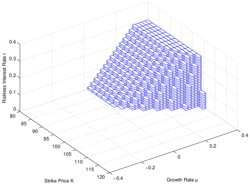
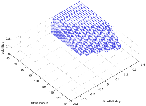
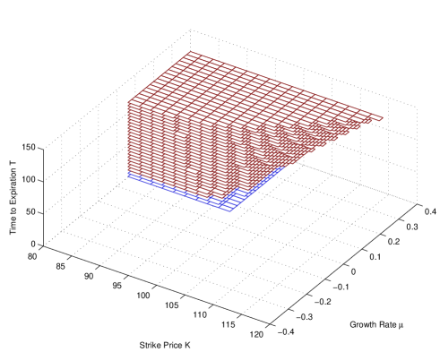
Figure 1: Compositions of $\mu$, $K$ $r$, $\sigma$, $T$ with probabilities larger than $50\%$.

Set the market factors as $S_{0}=100$, $K/S_{0}\in[0.8,1.2]$, $\mu\in[-0.4,0.4]$ per year. The compositions of $\left(K,\mu,r\right)$ are computed with $\sigma=0.1$ per year, $T=60$ days, $r\in[0.001,0.3]$ per year. The compositions of $\left(K,\mu,\sigma\right)$ are calculated with $r=0.05$ per year, $T=60$ days, $\sigma\in[0.001,0.2]$ per year. And the compositions of $\left(K,\mu,T\right)$ are calculated with $r=0.05$ per year, $\sigma=0.1$ per year, $T\in[1,120]$ days.

From figure (1), we can see that the probabilities of positive returns must be less than $50\%$, when the growth rates of stock prices are negative. The probabilities are on average beyond $50\%$ for in-the-money options, and below $50\%$ for out-of-the-money options, when the growth rates of stock prices are positive. The option holders will try to buy the options with probabilities beyond $50\%$, and not to buy the options with probabilities below $50\%$, which makes the market prices are on average larger than the BS values for in-the-money options, and less than the BS values for out-of-the-money options.

It is interesting to find that these theoretical predictions are consistent with the empirical observations of [2], where the market prices are on average lager than the BS values for in-the-money options, and less than the BS values for out-of-the-money options. Therefore the observed anomalies of BS values may be correlated with the growth rates of stock prices, and the probabilities of positive returns should be taken into account in derivative valuation.

3 Probability of Positive Return and Option Price

When there are transaction costs or other frictions, [13, 14, 15] show that the no-arbitrage conditions only place bounds on option prices, therefore the prices of options should be determined through equilibrium methods, rather than no-arbitrage models [4]. The financial market without friction has been discussed in the previous section, and the numerical investigations indicate that the BS values should be adjusted according to their probabilities of positive returns, therefore BS values are not the equilibrium prices of options.

An equilibrium argument can be applied to determine the fair price of option through the probability of positive return. If the probability of positive return is larger than the equilibrium level, the investors would try to buy this option until the option price increases to eliminate the extra possibility of positive return. And the investors would not buy the options with probabilities below the equilibrium level, until the option price decrease enough to compensate the risk of negative return. On the other hand, the requirements of probabilities to achieve positive returns may be different among the investors according to their attitudes to risk.

The option price can be deduced from (6), if the equilibrium probability $p$ is determined previously, and we have the following proposition.

Proposition 3.

In the Black-Scholes market, if the equilibrium probability of positive return is $p$, and $p<N(e_{1})$, the equilibrium price of a European call option is

$$C(p)=S_{0}e^{-\sigma\sqrt{T}N^{-1}(\frac{p}{N(e_{1})})+(\mu-r-\frac{1}{2}\sigma^{2})T}-e^{-rT}K.$$ (8)

Otherwise, the required probability of positive return is beyond the the probability of the option to be exercised, therefore $C(p)$ does not exist (NaN). Where $N^{-1}(\cdot)$ is the inverse function of the standard normal distribution function.

Remark 1.

From equation (8), we can find that the individual attitude to risk is important to option valuation. The true probability of an option to be exercised is $N(e_{1})$, and those investors, whose individual requirements for the probabilities of positive returns are beyond $N(e_{1})$, would not buy this option. As market prices should lie in the no-arbitrage bounds, the option price $C(p)$ will be modified as $\min\left\{0,S_{0}-e^{-rT}K\right\}\leq\tilde{C}(p)\leq S_{0}$.

Proposition 4.

In the Black-Scholes model, the equilibrium option price $C(p)$ is a decreasing function with respect to $p$.

Proof.

It is directly from equation (8). ∎

This proposition says that the investors, whose requirements for probabilities of positive returns are larger than $p$, would not buy the options with prices beyond $C(p)$. On the other hand, these investors will buy the options with prices below $C(p)$.

$K$	$80.00$	$82.00$	$84.00$	$86.00$	$88.00$	$90.00$	$92.00$	$94.00$	96.00	98.00	100.00	102.00	104.00	106.00	108.00	110.00	112.00
$BS$	$21.85$	$19.90$	$17.95$	$15.99$	$14.04$	$12.09$	$10.15$	$8.25$	6.43	4.74	3.29	2.11	1.25	0.68	0.34	0.15	0.06
$-0.25$	$21.85$	$19.90$	$17.95$	$15.99$	$14.04$	$12.08$	$10.13$	$8.18$	6.22	4.27	$NaN$	$NaN$	$NaN$	$NaN$	$NaN$	$NaN$	$NaN$
$-0.23$	$21.85$	$19.90$	$17.95$	$15.99$	$14.04$	$12.08$	$10.13$	$8.18$	6.22	4.27	$NaN$	$NaN$	$NaN$	$NaN$	$NaN$	$NaN$	$NaN$
$-0.21$	$21.85$	$19.90$	$17.95$	$15.99$	$14.04$	$12.08$	$10.13$	$8.18$	6.22	4.27	$NaN$	$NaN$	$NaN$	$NaN$	$NaN$	$NaN$	$NaN$
$-0.19$	$21.85$	$19.90$	$17.95$	$15.99$	$14.04$	$12.08$	$10.13$	$8.18$	6.22	4.27	$NaN$	$NaN$	$NaN$	$NaN$	$NaN$	$NaN$	$NaN$
$-0.17$	$21.85$	$19.90$	$17.95$	$15.99$	$14.04$	$12.08$	$10.13$	$8.18$	6.22	4.27	$NaN$	$NaN$	$NaN$	$NaN$	$NaN$	$NaN$	$NaN$
$-0.15$	$21.85$	$19.90$	$17.95$	$15.99$	$14.04$	$12.08$	$10.13$	$8.18$	6.22	4.27	2.32	$NaN$	$NaN$	$NaN$	$NaN$	$NaN$	$NaN$
$-0.13$	$21.85$	$19.90$	$17.95$	$15.99$	$14.04$	$12.08$	$10.13$	$8.18$	6.22	4.27	2.32	$NaN$	$NaN$	$NaN$	$NaN$	$NaN$	$NaN$
$-0.11$	$21.85$	$19.90$	$17.95$	$15.99$	$14.04$	$12.08$	$10.13$	$8.18$	6.22	4.27	2.32	$NaN$	$NaN$	$NaN$	$NaN$	$NaN$	$NaN$
$-0.09$	$21.85$	$19.90$	$17.95$	$15.99$	$14.04$	$12.08$	$10.13$	$8.18$	6.22	4.27	2.32	$NaN$	$NaN$	$NaN$	$NaN$	$NaN$	$NaN$
$-0.07$	$21.85$	$19.90$	$17.95$	$15.99$	$14.04$	$12.08$	$10.13$	$8.18$	6.22	4.27	2.32	0.36	$NaN$	$NaN$	$NaN$	$NaN$	$NaN$
$-0.05$	$22.30$	$20.34$	$18.39$	$16.43$	$14.45$	$12.43$	$10.31$	$8.18$	6.22	4.27	2.32	0.36	$NaN$	$NaN$	$NaN$	$NaN$	$NaN$
$-0.03$	$22.77$	$20.81$	$18.86$	$16.90$	$14.93$	$12.92$	$10.83$	$8.58$	6.22	4.27	2.32	0.36	$NaN$	$NaN$	$NaN$	$NaN$	$NaN$
$-0.01$	$23.24$	$21.29$	$19.33$	$17.38$	$15.41$	$13.41$	$11.34$	$9.13$	6.70	4.27	2.32	0.36	$NaN$	$NaN$	$NaN$	$NaN$	$NaN$
$0.01$	$23.72$	$21.76$	$19.81$	$17.85$	$15.89$	$13.90$	$11.85$	$9.68$	7.30	4.61	2.32	0.36	0.00	$NaN$	$NaN$	$NaN$	$NaN$
$0.03$	$24.20$	$22.24$	$20.29$	$18.33$	$16.37$	$14.39$	$12.36$	$10.22$	7.90	5.29	2.32	0.36	0.00	$NaN$	$NaN$	$NaN$	$NaN$
$0.05$	$24.68$	$22.72$	$20.77$	$18.82$	$16.86$	$14.88$	$12.86$	$10.75$	8.48	5.94	3.01	0.36	0.00	$NaN$	$NaN$	$NaN$	$NaN$
$0.07$	$25.16$	$23.21$	$21.25$	$19.30$	$17.34$	$15.37$	$13.36$	$11.28$	9.05	6.58	3.76	0.37	0.00	$NaN$	$NaN$	$NaN$	$NaN$
$0.09$	$25.65$	$23.69$	$21.74$	$19.78$	$17.83$	$15.86$	$13.86$	$11.80$	9.61	7.21	4.48	1.25	0.00	0.00	$NaN$	$NaN$	$NaN$
$0.11$	$26.13$	$24.18$	$22.23$	$20.27$	$18.32$	$16.35$	$14.37$	$12.32$	10.17	7.82	5.18	2.09	0.00	0.00	$NaN$	$NaN$	$NaN$
$0.13$	$26.62$	$24.67$	$22.72$	$20.76$	$18.81$	$16.85$	$14.87$	$12.84$	10.71	8.42	5.86	2.90	0.00	0.00	$NaN$	$NaN$	$NaN$
$0.15$	$27.12$	$25.16$	$23.21$	$21.25$	$19.30$	$17.34$	$15.37$	$13.35$	11.25	9.01	6.52	3.67	0.24	0.00	$NaN$	$NaN$	$NaN$
$0.17$	$27.61$	$25.66$	$23.70$	$21.75$	$19.80$	$17.84$	$15.87$	$13.87$	11.79	9.58	7.16	4.41	1.15	0.00	0.00	$NaN$	$NaN$
$0.19$	$28.11$	$26.15$	$24.20$	$22.25$	$20.29$	$18.34$	$16.37$	$14.38$	12.32	10.15	7.79	5.13	2.01	0.00	0.00	$NaN$	$NaN$
$0.21$	$28.61$	$26.65$	$24.70$	$22.75$	$20.79$	$18.84$	$16.87$	$14.89$	12.85	10.71	8.40	5.82	2.84	0.00	0.00	$NaN$	$NaN$
$0.23$	$29.11$	$27.15$	$25.20$	$23.25$	$21.29$	$19.34$	$17.38$	$15.40$	13.38	11.27	9.01	6.50	3.63	0.18	0.00	$NaN$	$NaN$
$0.25$	$29.61$	$27.66$	$25.71$	$23.75$	$21.80$	$19.84$	$17.88$	$15.91$	13.90	11.82	9.60	7.16	4.39	1.11	0.00	0.00	$NaN$

Table 1: BS values and $C(20\%)$ values for different growth rates. The strike prices are listed in the first row, and the second row are the BS values corresponding to those strike prices. The growth rates of stock price are listed in the first column, varying from $-0.25$ to $0.25$ per year. And the $C(20\%)$ values are reported according to the growth rates and strike prices respectively. NaN means that there is no possibility to achieve positive returns with probabilities larger than $20\%$ under the specified market.

$K$	$80.00$	$82.00$	$84.00$	$86.00$	$88.00$	$90.00$	$92.00$	$94.00$	96.00	98.00	100.00	102.00	104.00	106.00	108.00	110.00
$BS$	$21.85$	$19.90$	$17.95$	$15.99$	$14.04$	$12.09$	$10.15$	$8.25$	6.43	4.74	3.29	2.11	1.25	0.68	0.34	0.15
$-0.25$	$21.85$	$19.90$	$17.95$	$15.99$	$14.04$	$12.08$	$10.13$	$8.18$	$NaN$	$NaN$	$NaN$	$NaN$	$NaN$	$NaN$	$NaN$	$NaN$
$-0.23$	$21.85$	$19.90$	$17.95$	$15.99$	$14.04$	$12.08$	$10.13$	$8.18$	$NaN$	$NaN$	$NaN$	$NaN$	$NaN$	$NaN$	$NaN$	$NaN$
$-0.21$	$21.85$	$19.90$	$17.95$	$15.99$	$14.04$	$12.08$	$10.13$	$8.18$	$NaN$	$NaN$	$NaN$	$NaN$	$NaN$	$NaN$	$NaN$	$NaN$
$-0.19$	$21.85$	$19.90$	$17.95$	$15.99$	$14.04$	$12.08$	$10.13$	$8.18$	$NaN$	$NaN$	$NaN$	$NaN$	$NaN$	$NaN$	$NaN$	$NaN$
$-0.17$	$21.85$	$19.90$	$17.95$	$15.99$	$14.04$	$12.08$	$10.13$	$8.18$	$NaN$	$NaN$	$NaN$	$NaN$	$NaN$	$NaN$	$NaN$	$NaN$
$-0.15$	$21.85$	$19.90$	$17.95$	$15.99$	$14.04$	$12.08$	$10.13$	$8.18$	6.22	$NaN$	$NaN$	$NaN$	$NaN$	$NaN$	$NaN$	$NaN$
$-0.13$	$21.85$	$19.90$	$17.95$	$15.99$	$14.04$	$12.08$	$10.13$	$8.18$	6.22	$NaN$	$NaN$	$NaN$	$NaN$	$NaN$	$NaN$	$NaN$
$-0.11$	$21.85$	$19.90$	$17.95$	$15.99$	$14.04$	$12.08$	$10.13$	$8.18$	6.22	$NaN$	$NaN$	$NaN$	$NaN$	$NaN$	$NaN$	$NaN$
$-0.09$	$21.85$	$19.90$	$17.95$	$15.99$	$14.04$	$12.08$	$10.13$	$8.18$	6.22	$NaN$	$NaN$	$NaN$	$NaN$	$NaN$	$NaN$	$NaN$
$-0.07$	$21.85$	$19.90$	$17.95$	$15.99$	$14.04$	$12.08$	$10.13$	$8.18$	6.22	4.27	$NaN$	$NaN$	$NaN$	$NaN$	$NaN$	$NaN$
$-0.05$	$21.85$	$19.90$	$17.95$	$15.99$	$14.04$	$12.08$	$10.13$	$8.18$	6.22	4.27	$NaN$	$NaN$	$NaN$	$NaN$	$NaN$	$NaN$
$-0.03$	$21.85$	$19.90$	$17.95$	$15.99$	$14.04$	$12.08$	$10.13$	$8.18$	6.22	4.27	$NaN$	$NaN$	$NaN$	$NaN$	$NaN$	$NaN$
$-0.01$	$21.85$	$19.90$	$17.95$	$15.99$	$14.04$	$12.08$	$10.13$	$8.18$	6.22	4.27	$NaN$	$NaN$	$NaN$	$NaN$	$NaN$	$NaN$
$0.01$	$21.85$	$19.90$	$17.95$	$15.99$	$14.04$	$12.08$	$10.13$	$8.18$	6.22	4.27	2.32	$NaN$	$NaN$	$NaN$	$NaN$	$NaN$
$0.03$	$21.85$	$19.90$	$17.95$	$15.99$	$14.04$	$12.08$	$10.13$	$8.18$	6.22	4.27	2.32	$NaN$	$NaN$	$NaN$	$NaN$	$NaN$
$0.05$	$21.85$	$19.90$	$17.95$	$15.99$	$14.04$	$12.08$	$10.13$	$8.18$	6.22	4.27	2.32	$NaN$	$NaN$	$NaN$	$NaN$	$NaN$
$0.07$	$21.85$	$19.90$	$17.95$	$15.99$	$14.04$	$12.08$	$10.13$	$8.18$	6.22	4.27	2.32	$NaN$	$NaN$	$NaN$	$NaN$	$NaN$
$0.09$	$21.85$	$19.90$	$17.95$	$15.99$	$14.04$	$12.08$	$10.13$	$8.18$	6.22	4.27	2.32	0.36	$NaN$	$NaN$	$NaN$	$NaN$
$0.11$	$21.97$	$20.02$	$18.06$	$16.11$	$14.15$	$12.18$	$10.17$	$8.18$	6.22	4.27	2.32	0.36	$NaN$	$NaN$	$NaN$	$NaN$
$0.13$	$22.44$	$20.49$	$18.53$	$16.58$	$14.62$	$12.66$	$10.66$	$8.58$	6.33	4.27	2.32	0.36	$NaN$	$NaN$	$NaN$	$NaN$
$0.15$	$22.91$	$20.96$	$19.01$	$17.05$	$15.10$	$13.13$	$11.14$	$9.09$	6.89	4.40	2.32	0.36	$NaN$	$NaN$	$NaN$	$NaN$
$0.17$	$23.39$	$21.43$	$19.48$	$17.53$	$15.57$	$13.61$	$11.63$	$9.59$	7.43	5.03	2.32	0.36	$NaN$	$NaN$	$NaN$	$NaN$
$0.19$	$23.87$	$21.91$	$19.96$	$18.00$	$16.05$	$14.09$	$12.12$	$10.10$	7.97	5.64	2.91	0.36	0.00	$NaN$	$NaN$	$NaN$
$0.21$	$24.34$	$22.39$	$20.44$	$18.48$	$16.53$	$14.57$	$12.60$	$10.60$	8.50	6.23	3.61	0.36	0.00	$NaN$	$NaN$	$NaN$
$0.23$	$24.83$	$22.87$	$20.92$	$18.97$	$17.01$	$15.05$	$13.09$	$11.09$	9.03	6.80	4.29	1.23	0.00	$NaN$	$NaN$	$NaN$
$0.25$	$25.31$	$23.36$	$21.40$	$19.45$	$17.50$	$15.54$	$13.58$	$11.59$	9.54	7.37	4.93	2.04	0.00	$NaN$	$NaN$	$NaN$

Table 2: BS values and $C(50\%)$ values for different growth rates. The strike prices are listed in the first row, and the second row are the BS values corresponding to those strike prices. The growth rates of stock price are listed in the first column, varying from $-0.25$ to $0.25$ per year. And the $C(50\%)$ values are reported according to the growth rates and strike prices respectively. NaN means that there is no possibility to achieve positive returns with probabilities larger than $50\%$ under the specified market.

4 Comparisons of the Two Option Prices

4.1 Growth Rates and Biases of BS Values

In order to investigate the performance of the proposed method, set the market factors as $S_{0}=100$, $r=0.05$ per year, $\sigma=0.1$ per year, $T=60$ days, and calculate the call option prices for $K/S\in[0.8,1.15]$, $\mu\in[-0.25,0.25]$ per year, using both BS formula and the proposed method. The results are reported in table (1) and table (2) with respect to $p=20\%$ and $p=50\%$.

From table (1), we can find that the BS values are systematically larger than or equal to those $C(20\%)$ values for all of the strike prices, when the growth rates are between $-0.25$ to $-0.07$. For those deep in-the-money options, the BS values are gradually less than the $C(20\%)$ values, when the growth rates are larger than $-0.05$. For those slightly in-the-money options, the BS values are most likely larger than those $C(20\%)$ values, when the growth rates are between $-0.05$ to $-0.01$. When the growth rates are larger than $0.01$, the BS values of in-the-money options are all less than the $C(20\%)$ values. For those deep out-of-the-money options, the BS values are systematically larger than those $C(20\%)$ values. For those slightly out-of-the-money options, the BS values are less than the $C(20\%)$ values, when the growth rates are larger than $0.13$.

A similar phenomena is observed in table (2) with $p=50\%$. We can conclude that the values of proposed method are on average larger than the BS values for in-the-money options, and less than the BS values for out-of-the-money options in our numerical investigations. It is interesting to find that those theoretical observations are consistent with the empirical results of [2], where the market prices of options are on average larger than the BS values for in-the-money options, and less than the BS values for out-of-the-money options.

4.2 Implied Volatility

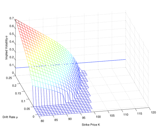
Figure 2: The surface of implied volatilities and the reference line.

As the influence of growth rate has been taken into account in the values of $C(p)$, it is possible to investigate the implied volatilities for different growth rates with respect to BS formula. Set the market factors as $S_{0}=100$, $T=60$ days, $\sigma=0.1$ per year, $r=0.05$ per year, $p=0.5$, $K/S\in[0.8,1.2]$, $\mu\in[-0.1,0.25]$ per year. The surface of implied volatilities for different $\mu$ is plotted in figure (2).

From figure (2), we can see that there is significant inconsistency of implied volatilities using the $C(50\%)$ values as market prices. The shape of the implied volatilities is similar to the empirical results of many authors, such as [6]. Therefore the growth rate of stock price should be used to explain the biases of BS formula, and the probabilities of positive returns should be taken into account in derivative valuation.

5 Conclusions and Discussions

The biases of Black-Scholes formula have been discussed widely for a long time, and many market factors have been used to explain the observed anomalies of BS values, such as strike price, volatility, time to expiration, bid-ask spread, trading volume, option open interest, transaction cost, etc. Although the growth rate is an important factor to describe the dynamics of stock prices, it is rarely discussed in the literature for the biases of BS formula. Most of the reason is that the physical growth rate of stock price is eliminated on the procedure of risk neural valuation, and the resulted option price is not correlated with the growth rate. The influence of growth rate on the biases of BS formula is investigated under the BS model, and it is found that the larger the growth rate, the more possible the option to be exercised with positive returns. Therefore the BS values are not the equilibrium prices, and the market prices need to be adjusted from their BS values to the equilibrium prices, according to the probabilities of positive returns.

An alternative valuation method for European call option is proposed in this paper. The probability of positive return is used to identify the risk of holding an option, and the equilibrium price of option will balance the requirements for probabilities of positive returns between the both parties in the transaction. The performance of BS formula and the proposed method are compared under the BS model, and it is found that the values of proposed method are on average larger than the BS values for in-the-money options, and less than the BS values for out-of-the-money options. These theoretical phenomenon are similar to the empirical results reported by [2], if we take the values of proposed method as the market prices.

The values of proposed method are also used to calculate the implied volatilities from BS formula. It is found that the shape of implied volatilities is similar to the empirical observations, such as [6]. From the biases of BS values and the shape of implied volatilities in our numerical investigations, we can conclude that there must be some similarity between the market prices and the values of proposed method, therefore the proposed valuation method may have some merit.

As the focus of this paper is to discuss the possibility to explain the observed anomalies of BS formula by the growth rate of stock price theoretically, the empirical performance of the proposed valuation method is not investigated in detail. Future research should investigate the empirical performance of the proposed method, and pay more attention to the mechanism of market equilibrium, when the probabilities of positive returns are taken into account in the investment decisions.

Appendix A The proof of Proposition 1

Proof.

The probability of positive return can be rewritten as

$$p(C) = Pr\left\{\left(S_{T}-K\right)^{+}-Ce^{rT}\geq 0|S_{T}-K\geq 0\right\}\cdot Pr\left\{S_{T}-K\geq 0\right\}$$ (9)

$$+Pr\left\{\left(S_{T}-K\right)^{+}-Ce^{rT}\geq 0|S_{T}-K<0\right\}\cdot Pr\left\{S_{T}-K<0\right\}$$

$$= Pr\left\{S_{T}\geq K\right\}\cdot Pr\left\{S_{T}\geq K+Ce^{rT}\right\}.$$

On the other hand, we have

$$Pr\left\{S_{T}\geq K\right\} = Pr\left\{S_{0}exp\left(\sigma W_{T}+\left(\mu-\frac{1}{2}\sigma^{2}\right)T\right)\geq K\right\}$$ (10)

$$= Pr\left\{\frac{-\sigma W_{T}}{\sigma\sqrt{T}}\leq\frac{\log\left(\frac{S_{0}}{K}\right)+(\mu-\frac{1}{2}\sigma^{2})T}{\sigma\sqrt{T}}\right\}$$

$$= N(e_{1}).$$

Following a similar procedure, we have

$$Pr\left\{S_{T}\geq K+Ce^{rT}\right\}=N(e_{2}),$$ (11)

and the desired result will follow. ∎

Appendix B The proof of Proposition 3

Proof.

When $p>N\left(e_{1}\right)$ is held, the inverse function $N^{-1}\left(\frac{p}{N\left(e_{1}\right)}\right)$ dose not exist. When $p<N\left(e_{1}\right)$ is held, from $p=N(e_{1})N(e_{2})$, we have $N\left(e_{2}\right)=\frac{p}{N\left(e_{1}\right)}$, and it follows that

$$e_{2}=N^{-1}\left(\frac{p}{N\left(e_{1}\right)}\right).$$ (12)

On the other hand, we have

$$e_{2}=\frac{\log\left(\frac{S_{0}}{K+Ce^{rT}}\right)+\left(\mu-\frac{1}{2}\sigma^{2}\right)T}{\sigma\sqrt{T}}.$$ (13)

Substituting (13) into (12), the desired result follows. ∎

References

References

- [1] Chiras, D. and Manaster, S., Journal of Financial Economics 5 (1978) 213.
- [2] Macbeth, J. and Merville, L., The Journal of Finance 5 (1979) 1173.
- [3] Rubinstein, M., The Journal of Finance 40 (1985) 455.
- [4] Longstaff, F. A., The Review of Financial Studies 4 (1995) 1091.
- [5] Thompson, J. and Williams, E., Journal of Post Keynesian Economics 2 (1999) 247.
- [6] Kuwahara, H. and Marsh, T. A., International Review of Finance 3 (2000) 195.
- [7] Isaenko, S., Economic Netes by Banca Monte dei Paschi di Siena SpA 1 (2007) 1.
- [8] Black, F. and Scholes, M., The Journal of Political Economy 81 (1973) 637.
- [9] Merton, R. C., Bell Journal of Economics and Management Science 4 (1973) 141.
- [10] Cox, J. C. and Ross, S. A., Journal of Financial Economics 3 (1976) 145.
- [11] Harrison, J. and Kreps, D. M., Journal of Economic Theory 20 (1979) 381.
- [12] Harrison, J. M. and Pliska, S. R., Stochastic Processes and their Applications 11 (1981) 261.
- [13] Perrakis, S. and Ryan, P. J., The Journal of Finance 39 (1984) 519.
- [14] Levy, H., The Journal of Finance 40 (1985) 1197.
- [15] Ritchken, P., The Journal of Finance 40 (1985) 1219.