Spontaneous chiral symmetry breaking on the lattice

Abstract:

Using lattice QCD we study the spectrum of low-lying fermion eigenmodes. According to the Banks-Casher relation, accumulation of the low-mode is responsible for the spontaneous breaking of chiral symmetry in the QCD vacuum. On the lattice we use the overlap fermion formulation that preserves exact chiral symmetry. This is essential for the study of low-lying eigenmode distributions. Through a detailed comparison with the expectations from chiral perturbation theory beyond the leading order, we confirm the senario of the spontaneous symmetry breaking and determine some of the low energy constants. We also discuss on other related physical quantities, which can be studied on the lattice with exact chiral symmetry.

1 Introduction

Spontaneous breaking of chiral symmetry is the most fundamental property of the vacuum of Quantum Chromodynamics (QCD). Once we assume that the chiral symmetry is spontaneously broken, we can derive many important relations in the phenomenology of strong interaction, such as the GMOR relation, Goldberger-Treiman relation, and other soft pion theorems, which are written in the language of chiral effective theory. The problem of how and why the spontaneous chiral symmetry breaking occurs remains a difficult question due to the non-perturbative dynamics of QCD.

Chiral symmetry of course plays a key role in the understanding of chiral symmetry breaking. In the flavor non-singlet sector of chiral symmetry, pion arises as the Nambu-Goldstone boson associated with the spontaneous symmetry breaking, while in the flavor-singlet sector the chiral symmetry is violated by the axial anomaly and is related to the topology of non-Abelian gauge theory. There are near-zero modes of quarks associated with the topological excitations; their accumulation in the vacuum leads to the symmetry breaking in the flavor non-singlet sector as indicated by the Banks-Casher relation. Therefore, the initial setup to study the chiral symmetry breaking should preserve both the flavor singlet and non-singlet chiral symmetries.

Lattice QCD is the most promising approach to solve the low-energy dynamics of QCD, but there is a problem in realizing the chiral symmetry on the lattice. The conventional Wilson-type fermions violate the chiral symmetry at the action level, and the discrimination between the physical effect of symmetry breaking and the lattice artifact cannot be done in a clear manner. On the other hand, the staggered fermions have a chiral symmetry but break the flavor symmetry. With these lattice fermions, the continuum limit has to be taken before analyzing the data with the continuum chiral effective theory.

Among other physical quantities, we are interested in extracting the chiral condensate $\langle\bar{q}q\rangle$, which is an order parameter of the chiral symmetry breaking. This is not easy because the scalar density operator $\bar{q}q$ has a power divergence of the form $m_{q}/a^{2}$ as the cutoff $1/a$ goes to infinity, hence the massless limit has to be taken to obtain physical result. (When the chiral symmetry is violated from the outset as in the Wilson-type fermions, the divergence is even stronger $1/a^{3}$.) The condensate however vanishes in the massless limit, as far as the space-time volume is kept finite. Therefore, the proper order of the limits is to take the infinite volume limit first and then the massless limit, which is called the thermodynamical limit. Thus, the study of symmetry breaking is numerically so demanding, and some theoretical guidance is required to control the limits. In QCD, the chiral perturbation theory (ChPT) provides such a theoretical framework.

This work is an attempt to simulate the QCD vacuum on the lattice with exact chiral symmetry. We use the overlap fermion formulation [1, 2], that exactly preserves chiral and flavor symmetries at finite lattice spacing and correctly reproduces the axial anomaly. We calculate the chiral condensate in various ways, which provides a good test of the chiral effective theory. In particular, we study the spectral density of the Dirac operator and compare it with ChPT at the next-to-leading order (NLO) of the chiral expansion. We also discuss a few other consequences of spontaneous symmetry breaking and related lattice calculations, which are made possible with exact chiral symmetry on the lattice.

These works have been done by the JLQCD and TWQCD collaborations. An overview of their recent physics results is found in [3].

2 Dirac spectrum and chiral symmetry breaking

The chiral symmetry breaking is induced by an accumulation of low-lying eigenstates of quark-antiquark pair, as indicated by the Banks-Casher relation [4]

$$\lim_{m\to 0}\lim_{V\to\infty}\rho(\lambda=0)=\frac{\Sigma}{\pi},$$ (1)

where $\rho(\lambda)$ denotes the eigenvalue density of the Dirac operator, $\rho(\lambda)\equiv(1/V)\sum_{k}\langle\delta(\lambda-\lambda_{k})\rangle$. The expectation value $\langle\cdots\rangle$ represents an ensemble average and $k$ labels the eigenvalues of the Dirac operator on a given gauge field background. On the right hand side of (1), $\Sigma$ is the chiral condensate, $\Sigma=-\langle\bar{q}q\rangle$, evaluated in the massless quark limit. In the free theory, we expect a scaling $\rho(\lambda)\sim\lambda^{3}$, which vanishes at $\lambda=0$, for a dimensional reason. The relation (1) implies that the spontaneous chiral symmetry breaking characterized by non-zero $\Sigma$ is related to the number of near-zero modes in a given volume after taking the thermodynamical limit.

Based on ChPT, more detailed forms of $\rho(\lambda)$ at finite $\lambda$, $V$ and $m$ have been obtained. This is achieved by evaluating the chiral condensate at imaginary value $i\lambda$ of valence quark mass, relying on the analytic continuation. The spectral function is thus obtained without explicitly treating the quark eigenstates.

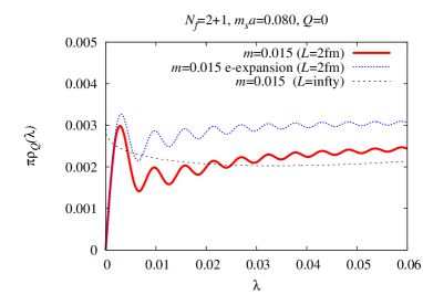
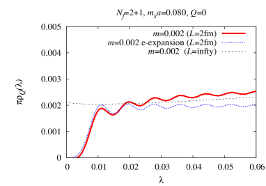
Figure 1: Theoretical expectation from [5] on the spectral function at $L\sim$ 2 fm. The left and right panels correspond to the pion mass around 300 MeV and 100 MeV, respectively. The curves correspond to the full NLO calculation (solid curve, red), the leading order result in the $\epsilon$-expansion (dashed curve, blue), and the result in the infinite volume (dotted curve, black) at NLO of the conventional $p$-expansion.

In this work, we use the most recent calculation by Damgaard and Fukaya [5], which is based on the conventional $p$-expansion of ChPT but includes an integral over zero-momentum modes of pion field, hence it is also consistent with the $\epsilon$-expansion. At NLO, they provide a formula for $\rho(\lambda)$ at finite $V$ and (non-degenerate) $m$. A typical example is shown in Figure 1 (left panel). The plot shows the spectral function $\rho(\lambda)$ at a given volume $V=L^{3}\times(3L)$ with $L\sim$ 2 fm and pion mass $m_{\pi}\sim$ 300 MeV. Within the leading order (LO) of the $\epsilon$-expansion, the spectral function is given by the dashed curve, which is equivalent to what one obtains from the chiral random matrix theory. It receives a finite volume correction at NLO and becomes the solid curve. Starting from the second peak of the oscillating curve, the spectral function is suppressed due to the pion-loop effects. In the infinite volume limit, we expect a smoother dotted curve, which contains a chiral logarithm.

The right panel of Figure 1 shows the spectral function in the $\epsilon$-regime. Here the lowest-lying eigenvalue is strongly suppressed by the fermion determinant as the quark mass is close to zero. The difference between LO and NLO in the $\epsilon$-expansion is less significant, since the system is in the $\epsilon$-regime.

Once we could calculate the spectral density on a finite volume lattice, we can extract $\Sigma$ and $1/F^{2}$. Essentially, $\Sigma$ determines the height of the distribution and $1/F^{2}$ the size of the NLO effects. The finite volume scaling should also be tested with more than one lattice volumes.

3 Lattice analysis of the spectral density

We use the lattice data obtained in the course of dynamical overlap fermion simulations by the JLQCD and TWQCD collaborations. The project mainly aimed at controlling the chiral extrapolation of physical quantities by realizing exact chiral and flavor symmetries in the lattice simulations. The use of the continuum ChPT is justified even at finite lattice spacings in contrast to other lattice fermion formulations, for which some modifications of ChPT with additional parameters is required. With the exact chiral symmetry, there have been several new physics applications proposed from the project [3].

We use the overlap-Dirac operator $D(0)\equiv(\rho/a)[1+X/\sqrt{X^{\dagger}X}]$ with the Wilson kernel $X\equiv aD_{W}-\rho$ [1, 2]. This fermion formulation exactly preserves a modified version of the chiral symmetry at finite lattice spacings [6]. The axial Ward-Takahashi identities are essentially the same as those in the continuum theory, and the index theorem is satisfied.

The large-scale Monte Carlo simulations had been made feasible by restricting the Markov chain in a given topological charge, since the overlap-Dirac operator has a discontinuity on the boarder of the topological charge, and the numerical costs grows as $V^{2}$ to treat the change of topology. This is achieved by introducing unphysical heavy Wilson fermions in the simulation [7]. Fixing topology induces a finite volume effect for any physical quantities, but corrections are possible using the general formulae developed in [9, 10]. For the calculation of the spectral function considered in this work, the fixed topology is an advantage rather than a disadvantage, as the ChPT formulae are given for fixed topological sectors.

At an early stage of the project, we performed simulations of two-flavor QCD at a lattice spacing $a\simeq$ 0.12 fm on a $16^{3}\times 32$ lattice. The simulation details are described in [8]. We took six values of sea quark mass in the range $m_{s}/6\sim m_{s}$, with $m_{s}$ the physical strange quark mass, to investigate the chiral extrapolation as discussed below. We also carried out a run in the $\epsilon$-regime with the quark mass around 3 MeV, in order to study the low-lying Dirac eigenvalue spectra, as discussed in the next section.

We then extended the work to 2+1-flavor simulations at a lattice spacing $a\simeq$ 0.11 fm on $16^{3}\times 48$ and $24^{3}\times 48$ lattices. We cover a similar range of (degenerate) up and down quark masses as in the two-flavor runs while taking two values of strange quark mass near its physical value. A dedicated run in the $\epsilon$-regime has also been performed with the up and down quark masses around 3 MeV while keeping the strange quark mass near the physical value. A preliminary report of these runs is found in [11].

At an early study of the eigenvalue spectrum, we use the distribution of the lowest-lying Dirac eigenvalue to extract $\Sigma$ in two-flavor QCD, by matching the distribution to the expectation from the chiral random matrix theory [12, 13]. In this method the relation to ChPT is established only at LO of the $\epsilon$-expansion, so that the result may contain significant finite volume effect, which is the NLO effect. This was signalled already by a slight inconsistency between $\Sigma$ obtained from the lowest and from the second lowest eigenvalues.

With the new formula [5], we can now consistently incorporate the NLO effects in the analysis. We use the 2+1-flavor data of spectral function in a wider region of the eigenvalue $\lambda$. Since the formula is valid also in the $p$-regime, we are able to include the $p$-regime lattices into the analysis.

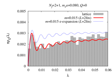
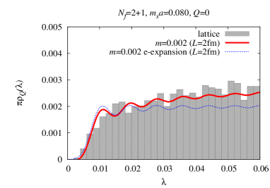
Figure 2: Lattice results for the spectral function (histogram) together with the LO (dashed, blue) and NLO (solid, red) curves. The left and right panels correspond to the pion mass around 300 MeV ($p$-regime) and 100 MeV ($\epsilon$-regime), respectively.

Figure 2 shows the results for the spectral function in 2+1-flavor QCD obtained on $16^{3}\times 48$ lattices. The global topological charge $Q$ is fixed to 0. The lattice data (histogram) are overlaid on the expectation from the NLO formula for both the $p$-regime (left panel) and $\epsilon$-regime (right panel). We observe that the NLO formula nicely reproduces the shape of the lattice data. The curves are drawn by fixing the parameters ($\Sigma$ and $F$) with the data for an integrated spectrum at two representative values of $\lambda$. Typically, one is taken near the top of the first peak, and the other is taken at $\lambda\sim$ 0.04, where the NLO effect is significant.

We have further tested the NLO formula by extending the calculation to a larger lattice. The finite volume scaling is tested with the data on a $24^{3}\times 48$ lattice in the $p$-regime. We find that the result for $\Sigma$ from this lattice is consistent with that on a smaller lattice after correcting the finite volume effect for both lattices. This implies that the lattice result scales as expected towards the thermodynamical limit.

From this analysis, we obtain $\Sigma$ at six values of up and down quark masses $m_{ud}$ while keeping the strange quark mass $m_{s}$ at its physical value. Thus, we obtain an “effective” value of $\Sigma$ at each sea quark mass, $\Sigma(m_{ud},m_{s})$. We extrapolate the results to the chiral limit of $m_{ud}$ using the NLO chiral expansion in two-flavor QCD [14]

$$\Sigma(m_{ud},m_{s})=\Sigma(0,m_{s})\left[1-\frac{3M_{\pi}^{2}}{32\pi^{2}F^{2}}\ln\frac{M_{\pi}^{2}}{F^{2}}+\frac{32L_{6}M_{\pi}^{2}}{F^{2}}\right]$$ (2)

as shown in Figure 3. (In the actual analysis, we use the formula including finite volume corrections.)

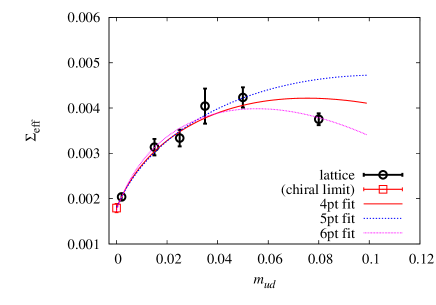
Figure 3: Chiral extrapolation of $\Sigma(m_{ud},m_{s})$ to the limit of vanishing up and down quark masses.

Since we have the data in the $\epsilon$-regime, which is very close to the chiral limit, the chiral extrapolation is stable against the change of the fitting region. We also attempt to use the 2+1-flavor formula at NLO, and find the result in the chiral limit is consistent.

After renormalizing to the $\overline{\mbox{MS}}$ scheme at 2 GeV using a non-perturbatively calculated renormalization factor [15], we obtain a preliminary result $\Sigma^{\overline{\mathrm{MS}}}(0,m_{s};\mathrm{2~{}GeV})=[243(4)(^{+16}_{-\ 0})\mathrm{~{}MeV}]^{3}$, where the second error represents an uncertainty due to the lattice scale. We also obtained $F$ and $L_{6}$ that are consistent with phenomenological analysis. For more details, see [16].

4 Other consequences of spontaneous symmetry breaking

The accumulation of the near-zero modes as seen in the spectral function is a direct measure of the spontaneous chiral symmetry breaking, as its infinite volume limit corresponds to the Banks-Casher relation. On the other hand, there are many other physical quantities that reflect the spontaneous breaking of chiral symmetry. In the following, we describe a few of them calculated on the same set of lattice simulations.

4.1 Topological susceptibility

Topological susceptibility $\chi_{t}\equiv\langle Q^{2}\rangle/V$ characterizes how much topological excitations are occurring in the QCD vacuum. Although the definition involves the global topological charge $Q$, the susceptibility itself is a local quantity and could be determined even when $Q$ is kept fixed [10]. Namely, $\chi_{t}$ can be extracted from topological charge density correlator as

$$\lim_{|x|\to\infty}\langle mP(x)mP(0)\rangle_{Q}=-\frac{1}{V}\left(\chi_{t}-\frac{Q^{2}}{V}+\cdots\right)+O(e^{-m_{\eta^{\prime}}|x|}),$$ (3)

where $mP(x)$ is a flavor-singlet pseudoscalar density operator related to the topological charge density through the axial-anomaly relation. When $Q=0$, this correlator approaches a negative constant at large separation $|x|$ after the excitation of the $\eta^{\prime}$ meson saturates. This is intuitively understood as follows. Since the global topological charge is fixed to zero, if we find a positive topological charge excitation at a space-time point $0$, then we have more chance to find a negative excitation at other points $x$ to keep the total to be zero.

This constant correlation is indeed observed in our work where we calculate the flavor-singlet pseudo-scalar correlator by maximally using the low-lying eigenmodes exactly calculated and stored on disks [17, 18]. We thus extract $\chi_{t}$ at each sea quark mass.

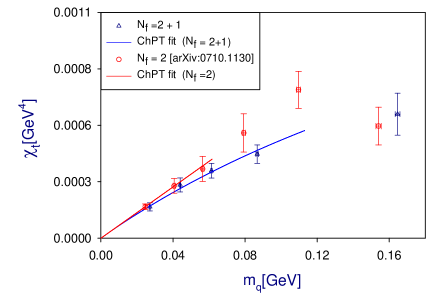
Figure 4: Topological susceptibility $\chi_{t}$ in 2 (circles) and 2+1-flavor (triangles) QCD as a function of up and down quark masses.

Sea quark mass dependence of $\chi_{t}$ is plotted in Figure 4. We observe a good agreement with the expectation from the chiral effective theory at the leading order, $\chi_{t}=\Sigma/(1/m_{u}+1/m_{d}+1/m_{s})$ [19]. ($m_{s}$ is sent to infinity for the two-flavor case.) It provides another method to extract $\Sigma$. Our result is $[247(3)(2)\mbox{~{}MeV}]^{3}$ (up to the error due to the scale setting), which is in agreement with the determination from the spectral function.

4.2 Vacuum polarization functions

The vacuum polarization function $\Pi_{J}^{(0,1)}(Q^{2})$ defined through

$$\int d^{4}xe^{iqx}\langle 0|J_{\mu}(x)J_{\nu}^{\dagger}(0)|0\rangle=(g_{\mu}q^{2}-q_{\mu}q_{\nu})\Pi_{J}^{(1)}(Q^{2})-q_{\mu}q_{\nu}\Pi_{J}^{(0)}(Q^{2})$$ (4)

for vector ($J=V$) or axial-vector ($J=A$) current is another probe of the spontaneous symmetry breaking. For example, the difference between vector and axial-vector channels is related to $f_{\pi}$ and $L_{10}$ (one of the NLO low energy constants in ChPT) as

$$f_{\pi}^{2} = -\lim_{Q^{2}\to 0}Q^{2}\left[\Pi_{V}^{(1+0)}(Q^{2})-\Pi_{A}^{(1+0)}(Q^{2})\right],$$ (5)

$$L_{10} = -\lim_{Q^{2}\to 0}\frac{\partial}{\partial Q^{2}}Q^{2}\left[\Pi_{V}^{(1+0)}(Q^{2})-\Pi_{A}^{(1+0)}(Q^{2})\right],$$ (6)

which are called the Weinberg sum rules [20]. Another interesting quantity is the electromagnetic mass difference of pion, which is expressed as [21]

$$\Delta m_{\pi}^{2}=-\frac{3\alpha_{EM}}{4\pi f_{\pi}^{2}}\int_{0}^{\infty}dQ^{2}Q^{2}\left[\Pi_{V}^{(1+0)}(Q^{2})-\Pi_{A}^{(1+0)}(Q^{2})\right],$$ (7)

in the limit of massless pion. Since the combination $\langle VV-AA\rangle$ vanishes unless the chiral symmetry is broken, these quantities signal the chiral symmetry breaking.

Figure 5: Difference of the vacuum polarization functions, $\Pi_{V}^{(1)}(Q^{2})-\Pi_{A}^{(1)}(Q^{2})$, multiplied by $Q^{2}$. Data are shown for different quark masses; the chiral limit is also plotted by solid (linear extrapolation) and dashed (chiral logs) curves.

For the lattice calculation of these quantities, exact chiral symmetry is essential, since we have to extract a tiny difference between the vector and axial-vector channels. We extracted the difference $\Pi_{V}^{(1)}(Q^{2})-\Pi_{A}^{(1)}(Q^{2})$ successfully, using the overlap fermion on the lattice [22], as shown in Figure 5. The intercept and slope of $Q^{2}[\Pi_{V}^{(1)}(Q^{2})-\Pi_{A}^{(1)}(Q^{2})]$ at $Q^{2}=0$ correspond to $f_{\pi}^{2}$ and $L_{10}$, respectively, and the integral over $Q^{2}$ gives $\Delta m_{\pi}^{2}$. The results clearly show that the spontaneous symmetry breaking induces these physical quantities as expected. By further improving the numerical data especially in the low $Q^{2}$ region, we will be able to precisely extract these quantities.

Another use of the vacuum polarization function is an extraction of the strong coupling constant by matching the lattice data with the OPE expression in the perturbative regime [23].

4.3 Pion mass and decay constant

ChPT is organized as an expansion in terms of small $m_{\pi}^{2}$ and $p^{2}$, but the region of convergence of this chiral expansion is not known a priori. Using lattice QCD, one can test the expansion and identify the region of convergence. With the exact chiral symmetry, the test is conceptually cleanest, since no additional terms to describe the violation of chiral symmetry has to be introduced. (With other fermion formulations, this is not the case. The unknown correction terms are often simply ignored.)

For the pion mass $m_{\pi}$ and decay constant $f_{\pi}$, the expansion is given as

$$\frac{m_{\pi}^{2}}{m_{q}} = 2B\left[1+\frac{1}{2}x\ln x+c_{3}x+O(x^{2})\right],$$ (8)

$$f_{\pi} = f\left[1-x\ln x+c_{4}x+O(x^{2})\right],$$ (9)

where $m_{\pi}$ and $f_{\pi}$ denote the quantities after the corrections while $m$ and $f$ are them at the leading order. The expansions (8) and (9) may be written in terms of either $x\equiv 2m^{2}/(4\pi f)^{2}$, $\hat{x}\equiv 2m_{\pi}^{2}/(4\pi f)^{2}$, or $\xi\equiv 2m_{\pi}^{2}/(4\pi f_{\pi})^{2}$ (we use a notation of $f_{\pi}$ = 131 MeV). They all give an equivalent description at this order, while the convergence behavior may depend on the expansion parameter.

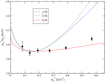
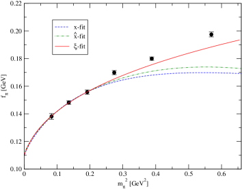
Figure 6: Comparison of chiral expansion in terms of $x$, $\hat{x}$ and $\xi$. The plots represent $m_{\pi}^{2}/m_{q}$ (left) and $f_{\pi}$ (right). Fits of the three lightest data points with the NLO ChPT formulae (8) and (9) are shown.

Figure 6 shows the comparison of different expansion parameters [24] in two-flavor QCD. The fit curves are obtained by fitting three lightest data points with the three expansion parameters, which provide equally precise description of the data in the region of the fit. If we look at the heavier quark mass region, however, it is clear that only the $\xi$-expansion gives a reasonable function and others miss the data points largely. This clearly demonstrates that at least for these quantities the convergence of the chiral expansion is much better with the $\xi$-parameter than with the other conventional choices. This is understood as an effect of resummation of the chiral expansion by the use of the “renormalized” quantities $m_{\pi}^{2}$ and $f_{\pi}$. In fact, only with the $\xi$-expansion we could fit the data including the kaon mass region with the next-to-next-to-leading (NNLO) formulae [24].

Whether or not ChPT can be used for kaon is an important question and potentially has a strong impact on the light hadron phenomenology. To investigate this question, we are currently extending the analysis to 2+1-flavor QCD [25, 26].

5 Conclusions

In this talk, I demonstrate that the scenario of the spontaneous chiral symmetry breaking in the QCD vacuum is confirmed by lattice QCD simulations with exact chiral symmetry. In the calculation of the Dirac operator eigenvalue spectrum, the expectations from ChPT is precisely tested including the NLO effects.

With the use of exact chiral symmetry, new possibilities to extract physics from lattice QCD calculations have been opened. They include the precise calculation of the topological susceptibility, the vacuum polarization functions, and a theoretically clean test of chiral expansion in pion mass and decay constant. From the project, there are several other interesting calculations of various physical quantities, such as $B_{K}$ [27], meson correlators in the $\epsilon$-regime [28], nucleon $\sigma$-term and strange quark content [29], and pion form factors [30].

Some of the applications discussed in this talk have been left without so much progress since the early days of QCD (or even before). At last, numerical simulation of lattice QCD has caught up theoretical conjectures made in 1960s and 70s, but now starting from the first-principles.

I thank the members of JLQCD/TWQCD for fruitful collaborations. The author is supported in part by Grant-in-aid for Scientific Research (No. 21674002).

References

- [1] H. Neuberger, Phys. Lett. B 417, 141 (1998) [arXiv:hep-lat/9707022].
- [2] H. Neuberger, Phys. Lett. B 427, 353 (1998) [arXiv:hep-lat/9801031].
- [3] S. Hashimoto, arXiv:0811.1257 [hep-lat].
- [4] T. Banks and A. Casher, Nucl. Phys. B 169, 103 (1980).
- [5] P. H. Damgaard and H. Fukaya, JHEP 0901, 052 (2009) [arXiv:0812.2797 [hep-lat]].
- [6] M. Luscher, Phys. Lett. B 428, 342 (1998) [arXiv:hep-lat/9802011].
- [7] H. Fukaya et al. [JLQCD Collaboration], Phys. Rev. D 74 (2006) 094505 [arXiv:hep-lat/0607020].
- [8] S. Aoki et al. [JLQCD Collaboration], Phys. Rev. D 71 (2008) 014508 [arXiv:0803.3197 [hep-lat]].
- [9] R. Brower, S. Chandrasekharan, J. W. Negele and U. J. Wiese, Phys. Lett. B 560 (2003) 64 [arXiv:hep-lat/0302005].
- [10] S. Aoki, H. Fukaya, S. Hashimoto and T. Onogi, Phys. Rev. D 76 (2007) 054508 [arXiv:0707.0396 [hep-lat]].
- [11] H. Matsufuru et al. [JLQCD and TWQCD Collaborations], PoS LAT2008 (2008) 077.
- [12] H. Fukaya et al. [JLQCD Collaboration], Phys. Rev. Lett. 98 (2007) 172001 [arXiv:hep-lat/0702003].
- [13] H. Fukaya et al. [JLQCD and TWQCD Collaborations], Phys. Rev. D 76 (2007) 054503 [arXiv:0705.3322 [hep-lat]].
- [14] J. Gasser and H. Leutwyler, Annals Phys. 158, 142 (1984).
- [15] J. Noaki et al., arXiv:0907.2751 [hep-lat].
- [16] H. Fukaya et al. [JLQCD collaboration], arXiv:0911.5555 [hep-lat].
- [17] S. Aoki et al. [JLQCD and TWQCD Collaborations], Phys. Lett. B 665 (2008) 294 [arXiv:0710.1130 [hep-lat]].
- [18] T. W. Chiu et al. [JLQCD and TWQCD Collaborations], PoS LAT2008 (2008) 072; arXiv:0810.0085 [hep-lat].
- [19] H. Leutwyler and A. V. Smilga, Phys. Rev. D 46 (1992) 5607.
- [20] S. Weinberg, Phys. Rev. Lett. 18 (1967) 507.
- [21] T. Das, G. S. Guralnik, V. S. Mathur, F. E. Low and J. E. Young, Phys. Rev. Lett. 18 (1967) 759.
- [22] E. Shintani et al. [JLQCD Collaboration], Phys. Rev. Lett. 101, 242001 (2008) [arXiv:0806.4222 [hep-lat]].
- [23] E. Shintani et al. [JLQCD Collaboration and TWQCD Collaboration], Phys. Rev. D 79, 074510 (2009) [arXiv:0807.0556 [hep-lat]].
- [24] J. Noaki et al. [JLQCD and TWQCD Collaborations], arXiv:0806.0894 [hep-lat].
- [25] J. Noaki et al. [JLQCD and TWQCD collaborations], PoS LAT2008 (2008) 107; arXiv:0810.1360 [hep-lat].
- [26] J. Noaki et al. [JLQCD and TWQCD Collaborations], PoS LAT2009, 096 (2009) [arXiv:0910.5532 [hep-lat]].
- [27] S. Aoki et al. [JLQCD Collaboration], Phys. Rev. D 77 (2008) 094503 [arXiv:0801.4186 [hep-lat]].
- [28] H. Fukaya et al. [JLQCD collaboration], Phys. Rev. D 77, 074503 (2008) [arXiv:0711.4965 [hep-lat]].
- [29] H. Ohki et al., Phys. Rev. D 78, 054502 (2008) [arXiv:0806.4744 [hep-lat]].
- [30] S. Aoki et al. [JLQCD Collaboration and TWQCD Collaboration], Phys. Rev. D 80, 034508 (2009) [arXiv:0905.2465 [hep-lat]].