Evidence for departure from a power-law flare size distribution for a small solar active region

Abstract

Active region 11029 was a small, highly flare-productive solar active region observed at a time of extremely low solar activity. The region produced only small flares: the largest of the $>70$ Geostationary Observational Environmental Satellite (GOES) events for the region has a peak $1$–$8\mbox{\AA}$ flux of $2.2\times 10^{-6}\,{\rm W}\,{\rm m}^{-2}$ (GOES C2.2). The background-subtracted GOES peak-flux distribution suggests departure from power-law behavior above $10^{-6}\,{\rm W}\,{\rm m}^{-2}$, and a Bayesian model comparison strongly favors a power-law plus rollover model for the distribution over a simple power-law model. The departure from the power law is attributed to this small active region having a finite amount of energy. The rate of flaring in the region varies with time, becoming very high for two days coinciding with the onset of an increase in complexity of the photospheric magnetic field. The observed waiting-time distribution for events is consistent with a piecewise-constant Poisson model. These results present challenges for models of flare statistics and of energy balance in solar active regions.

1 Introduction

Solar flares are dynamic events in the Sun’s outer atmosphere, the corona, involving the explosive release of magnetic energy in active regions around sunspots. Large solar flares may produce hazardous local space weather conditions but these events are relatively infrequent, even at solar maximum (e.g. Odenwald, Green, & Taylor 2006; Hudson 2007). Small solar flares are much more common, and may also cause space-weather effects (e.g. Howard & Tappin 2005; Yermolaev et al. 2005). Many details of the flare mechanism remain poorly understood (e.g. Schrijver 2009), although the accepted model is magnetic reconnection (e.g. Priest & Forbes 2002). Because individual solar flares exhibit great variety, attention has often focused on the statistics of multiple events to try to understand the phenomenon (e.g. Smith & Smith 1963).

An important statistical property of flares is the appearance of a power law in the frequency-size distribution (e.g. Akabane 1956; Hudson 1969), i.e. the number $f(S)$ of flares observed per unit size $S$ and per unit time is distributed according to:

$$f(S)=AS^{-\gamma}.$$ (1)

By size we mean some measure of the magnitude of the event, for example the peak radiated flux in a short-wavelength band. In equation (1) the power-law index $\gamma$ is a constant, typically found to be in the range $1.5$–$2$ (the exact value depends on the chosen measure of size). The factor $A$ determines the mean rate of events during an observation period, and may be formally written

$$A=\lambda_{1}(\gamma-1)S_{1}^{\gamma-1},$$ (2)

where $\lambda_{1}$ is the mean rate above size $S_{1}$.

The power-law frequency-energy distribution appears to be universal, in the sense that the same power-law index is observed from the Sun at different times (e.g. Hudson 1991; Aschwanden, Dennis & Benz 1998; Su et al. 2006; Christe et al. 2008), although the mean rate of flaring varies substantially. The same index is also observed for different individual active regions (Wheatland 2000a). However, an upper limit to the size distribution (1) is required to ensure that the mean size of events is finite (assuming $\gamma<2$). Since the energy of a flare is expected to scale with size, this represents the physical constraint that there is a finite amount of magnetic free energy available for flaring. However, it has proven difficult to identify this limit in observed frequency-size distributions (e.g. Hudson 2007), and a departure from the power law has not been demonstrated for individual active regions. Statistical evidence has been presented for an upper limit to the size of flares from active regions with small sunspot areas based on a large sample of small regions (Kucera et al. 1997). Proxies for the Solar Energetic Particle spectrum also provide indirect evidence for a cut-off in the spectrum at large fluences (e.g. Lingenfelter & Hudson 1980). The search for departures from the flare frequency-size distribution at large event sizes may be complicated by detector saturation effects associated with big events (e.g. Thomson et al. 2004).

A second statistical property of flares of interest is the waiting-time distribution, or the distribution of times between flares, which is related to the constant $A$ in equations (1) and (2). Results for the waiting-time distribution have proven more ambiguous than for the frequency-size distribution, with a variety of functional forms reported (e.g. Pearce et al. 1993; Biesecker 1994; Wheatland et al. 1998; Boffetta et al. 1999; Moon et al. 2001; Wheatland 2001; Moon et al. 2002). This suggests that the distribution is time-dependent (Wheatland & Litvinenko 2002) and sensitive to event selection procedures (e.g. Wheatland 2001; Buchlin et al. 2005; Paczuski et al. 2005; Baiesi et al. 2006)

Waiting times in individual active regions often follow a simple exponential distribution corresponding to flares occurring as independent events with a constant mean rate (a Poisson process in time), or a distribution consisting of a sum of exponentials corresponding to distinct intervals with different rates (e.g. Moon et al. 2001; Wheatland 2001). A suitable model is then a piecewise-constant Poisson process, with a waiting-time distribution (Wheatland & Litvinenko 2002)

$$P(\Delta t)=\sum_{i}\frac{n_{1i}}{N}\lambda_{1i}{\rm e}^{-\lambda_{1i}\Delta t},$$ (3)

where $\Delta t$ denotes a waiting time, $n_{1i}=\lambda_{1i}t_{i}$ is the number of events above size $S_{1}$ corresponding to a rate $\lambda_{1i}$ which persists for an interval $t_{i}$, and where $N=\sum_{i}n_{1i}$ is the total number of events. For events over longer periods of time including many active regions, a power-law tail is observed in the waiting-time distribution (Boffetta et al. 1999). This also may be explained in terms of the time-dependent Poisson model (Wheatland 2000b; Wheatland & Litvinenko 2002), although some authors have argued for an intrinsic significance to the power law (e.g. Lepreti et al. 2001).

The observed event distributions have motivated models, in particular to account for the power-law frequency-size distribution. A popular model is the avalanche picture (Lu & Hamilton 1991; Charbonneau et al. 2001), which describes a flaring active region via a cellular automaton model (a field on a grid or lattice) which is continuously driven and achieves a self-organised critical state. A flare consists of an avalanche of local energy release events which trigger one another. Avalanche models produce a power-law frequency-size distribution, where size is the field energy $E_{F}$, below an upper rollover defined by the finite grid size $L$ (Lu et al. 1993; Wheatland & Sturrock 1996). The frequency-energy distribution was parameterized by Lu et al. (1993) using the power-law plus exponential form:

$$f(E_{F})\propto E_{F}^{-\gamma}{\rm e}^{-E_{F}/E_{r}},$$ (4)

where the rollover energy $E_{r}$ was found to scale as $E_{r}\propto L^{\beta}$, with $\beta\approx 3.9$. Avalanche models also produce exponential waiting-time distributions (e.g. Biesecker 1994; Wheatland et al. 1998), although time-dependent driving alters this (e.g. Norman et al. 2001).

Another approach to modeling flare event statistics involves describing the energy balance in a flaring active region in terms of energy input and loss (e.g. Rosner & Vaiana 1978; Litvinenko 1994; Craig 2001). A general model of this kind was presented in Wheatland & Glukhov (1998), and developed in Wheatland (2008; 2009). Active regions are assumed to have a free energy $E=E(t)$ which evolves in time $t$ due to deterministic energy input at a rate $\beta(E,t)$, and due to random downwards jumps from energy $E$ to $E^{\prime}$ (flares) at a rate described by a transition function $\alpha(E,E^{\prime},t)$. The resulting stochastic jump transition model may be formulated either as a master equation for the energy distribution $P(E,t)$ (Wheatland 2008), or as a stochastic differential equation for $E(t)$ (Wheatland 2009). In the steady state (i.e. for a constant driving rate and a constant total mean rate of flaring), the model can reproduce the observed power-law frequency size distribution, below an upper rollover defined approximately by the mean energy $\overline{E}$ of the steady-state distribution $P(E)$. Flares with energy $\gg\overline{E}$ are not observed because the active region is unlikely to have sufficient energy to produce them. The model waiting-time distribution is exponential provided $\overline{E}$ is sufficiently large that large flares are unlikely to significantly deplete the free energy of the system. In that case the total mean rate of flaring is approximately independent of energy, and hence does not vary in time, as the active region energy varies. This produces a Poisson waiting-time distribution. The stochastic jump transition model, although idealised, helps to clarify ideas of energy storage and release in flares, and their relationship to the flare frequency-energy and waiting-time distributions.

Studies of flares statistics often use the soft X-ray event lists generated by the US Space Weather Prediction Center, which are derived from whole-Sun $1$–$8\,\mbox{\AA}$ flux measurements from the Geostationary Observational Environmental (GOES) satellites. The peak flux of GOES events is routinely used to classify flares: very small flares are labelled A and B class (peak fluxes exceeding $10^{-8}\,{\rm W}\,{\rm m}^{-2}$ and $10^{-7}\,{\rm W}\,{\rm m}^{-2}$ respectively); small and medium flares are labelled C and M class (peak fluxes above $10^{-6}\,{\rm W}\,{\rm m}^{-2}$ and $10^{-5}\,{\rm W}\,{\rm m}^{-2}$ respectively); and large flares are labelled X class (peak flux above $10^{-4}\,{\rm W}\,{\rm m}^{-2}$). A numerical suffix is used to indicate a multiplicative factor, so that C$3.1$ indicates a peak flux of $3.1\times 10^{-6}\,{\rm W}\,{\rm m}^{-2}$. The recorded peak fluxes are not background-subtracted.

A recent period of extremely low solar activity (e.g. Livingston & Penn 2009; Salabert et al. 2009) has afforded a unique opportunity to study solar flares occurring in individual active regions with low levels of background emission from other regions on the disk. In this paper we examine a remarkable sequence of events in active region AR 11029 observed from 25 Oct 2009 to 1 Nov 2009. This small new-cycle sunspot region produced over 70 small soft X-ray flares in a dynamic one-week burst of activity, during which time it was the only flare-producing active region on the Sun. The absence of X-ray emission from other regions on the Sun at this time permits careful inspection of the statistics of GOES events for the region, including background subtraction of the peak flux. The key question addressed here is whether a small, highly flare-productive active region still exhibits a featureless power law in its flare frequency-size distribution, or whether it is possible to identify a departure from the power law at large flare sizes, corresponding perhaps to the region containing a finite amount of energy. It is also of interest to examine the waiting-time distribution for such a region, again taking advantage of the low levels of background emission, to see how the flaring rate varies in time.

The sections of the paper are divided as follows. Section 2 describes the observations of the region. Section 3 presents analysis, with section 3.1 describing the procedure of background subtraction of the peak fluxes, and sections 3.2 and 3.3 describing the analysis and modeling of the frequency-peak flux distribution and the waiting-time distribution respectively. Section 4 discussed the results, and the appendices present the methods of Bayesian inference for a power law and for a power law with an upper rollover used in section 3.2.

2 Observations

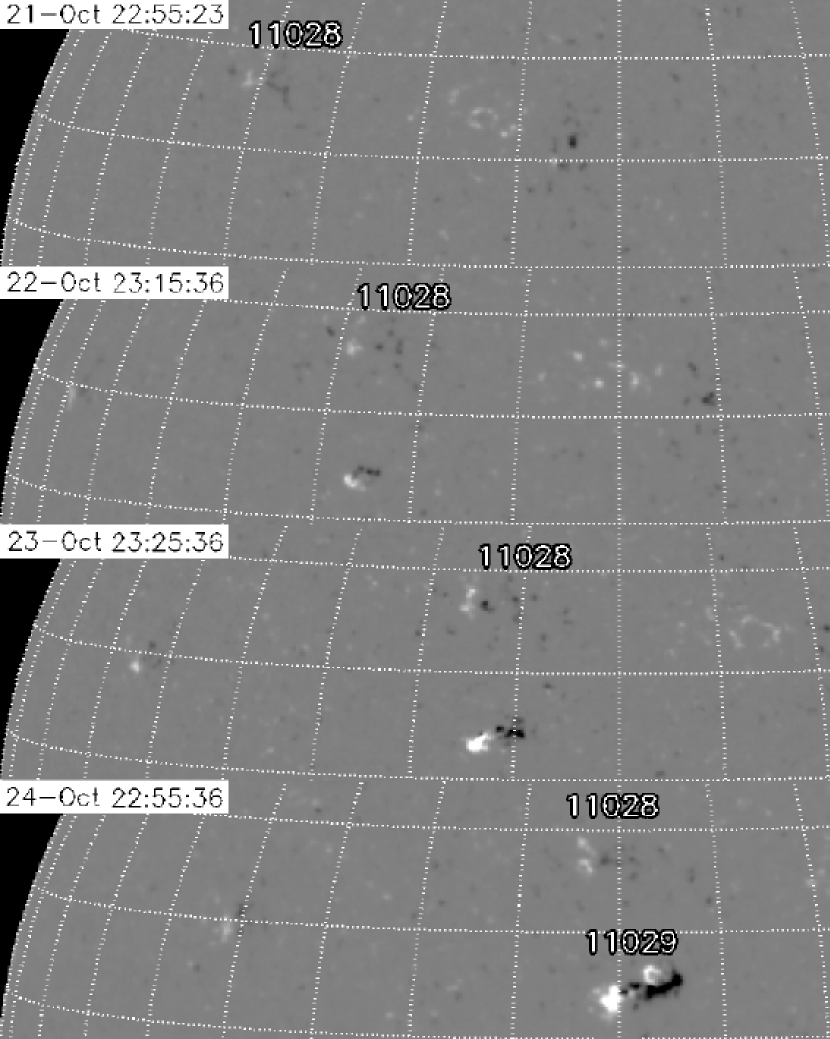
Figure 1: Collage of four Global Oscillations Network Group (GONG) magnetograms showing the emergence of AR 11029 and its development on the disk from 21 Oct 2009 (upper panel) to 24 Oct 2009 (lower panel). Active region 11028, also shown, was a simple $\beta$-region and did not flare. (Images from www.solarmonitor.org.)

Solar active region AR 11029 emerged on the disk on 21–22 Oct 2009 and developed sunspots on 24 Oct. Figure 1 shows a sequence of daily Global Oscillations Network Group (GONG) magnetograms for that period of time and illustrates the emergence of the region and its rapid evolution. The region grew in size and magnetic complexity as it crossed the disk, arriving at the west limb on 1 Nov. However the region remained relatively small: the sunspot areas recorded in the US National Weather Service/National Oceanic and Atmospheric Administration (NWS/NOAA) Solar Region Summaries are all $<400$ millionths of a hemisphere. Initially the region had a simple bipolar magnetic configuration and hence was given the Mount Wilson classification $\beta$. It developed into a $\beta$–$\gamma$ region (a more complex bipolar configuration such that a single line cannot be drawn to separate the polarities) for the period 26 to 29 Oct, and then returned to a $\beta$ configuration on 30 Oct.

The photospheric magnetic field of AR 11029 had the polarity orientation associated with the solar cycle 24, being a northern region with a leading negative polarity, although it appeared at an intermediate latitude (around 15 deg). At the time of writing (late 2009) there have been relatively few new cycle regions, and the interval of minimum since the peak of the last cycle, around 2001, has been longer and quieter than anticipated, with 2008 and 2009 featuring long stretches of days without sunspots (e.g. Livingston & Penn 2009; Salabert et al. 2009).

Although small, AR 11029 was highly flare productive. The GOES soft X-ray event lists compiled by the US SWPC (discussed in section 1) list 73 small flares for the interval 24 Oct to 1 Nov. In the SWPC lists, not all these events are attributed to AR 11029. However, the active region identification in the GOES event lists is quite incomplete: many events lack an associated location and active region number. (The identification is dependent on ground-based optical observations, and presumably locations are missing when there are no available optical observations.) Inspection of the SolarSoft Latest Events archive produced by the Lockheed Martin Solar & Astrophysics Laboratory, which includes Solar and Heliospheric Observatory Extreme Ultraviolet Imaging Telescope (SOHO/EIT) image sequences for each event, confirms that all 73 events originate in AR 11029. The flares are all small (one A-class event, 60 B-class events, and 11 C-class events), with the largest being C2.2. Table 1 summarises the daily behavior of the active region, and lists the numbers of flares observed per day. The region was particularly flare productive on 26 Oct and 27 Oct, the first two days of assignment of the magnetic classification $\beta$–$\gamma$.

Figure 2 illustrates the activity observed in AR 11029. The upper panel shows the one-minute GOES $1$–$8\,\mbox{\AA}$ flux values versus time from 23 Oct to 3 Nov, in a log-linear representation. Prior to the emergence of AR 11029 the X-ray flux was at the base level for the detector, and it returned to this value when the region rotated off the disk. This suggests that all $1$–$8\,\mbox{\AA}$ emission from the Sun in this interval originates from AR 11029, providing observation conditions which are close to ideal for identification of X-ray events from this region. The top panel of Figure 2 may be regarded as a soft X-ray light-curve for AR 11029. The lower panel of Figure 2 illustrates the GOES events identified by the US SWPC for the region, in a schematic diagram showing the peak flux of each event versus the peak time, with a vertical line drawn for each event. The event lists provide a start time, a peak time, and an end time for each event, as well as a peak flux. In the analysis in this paper the peak time is used to represent the event time. The lower panel of Figure 2 shows an initial interval with a low flaring rate (prior to 26 Oct), two days of intense flaring (26 Oct to 27 Oct, inclusive), and then a third interval with a low flaring rate.

3 Analysis

3.1 Background subtraction

The upper panel of Figure 2 illustrates issues associated with GOES event selection and background emission (Wheatland 2001). Even for a small active region observed at a time when there are no other X-ray emitting regions on the disk, a period of flaring is seen to raise the soft X-ray background by more than an order of magnitude. The SWPC events in the lower panel are selected against the time-varying background, and the peak fluxes shown are not background subtracted. The time-varying background leads to incompleteness in the event lists. The start of a GOES event is defined by four monotonically increasing one-minute flux values that produce a $40\%$ enhancement over the initial flux. At times of high background flux, small events fail to produce a $40\%$ enhancement over the background and are omitted. The absence of background-subtraction leads to time-dependent event definitions, so that events with the same intrinsic peak flux are assigned different peak fluxes at different times.

The absence of background subtraction for the peak fluxes is particularly important for small events, in which case the background is a substantial contributor to the event peak flux. To study the frequency-peak flux distribution, we background subtract each peak flux, using the one-minute GOES flux values. For each event the flux values prior to the start time $t_{\rm s}$ are averaged over an interval equal to the rise time $t_{\rm p}-t_{\rm s}$ of the event, where $t_{\rm p}$ is the peak time. The resulting flux is taken as the background estimate, and is subtracted off the peak flux value for the analysis in sections 3.2 and 3.3. This method of background subtraction is a suitable simple method. Any approach to background subtraction faces the problem of (unknown) variation in the background between the start time of an event and the peak time. The chosen approach is intended to capture typical variation over the relevant time scale for which the background is unknown (the rise time), and to provide a representative background flux.

Figure 3 illustrates the procedure and the results. The upper panel shows the first event from AR 11029, which occurred around 20:00 UT on 24 Oct. The one-minute flux values are shown versus time (solid curve), with the three vertical dotted lines indicating $t_{\rm s}$, $t_{\rm p}$, and $t_{\rm e}$ (the end time) for the event, as given by the SWPC event lists. The averaging interval is the interval to the left of the first vertical line, and the resulting background estimate is shown by the dotted horizontal line. This event is assigned a peak flux $1.6\times 10^{-7}\,{\rm W}\,{\rm m}^{-2}$ in the SWPC event lists (B1.6). The background estimate is $3.11\times 10^{-8}\,{\rm W}\,{\rm m}^{-2}$, so the resulting background-subtracted peak flux is $1.29\times 10^{-7}\,{\rm W}\,{\rm m}^{-2}$ (B1.3). The lower panel of Figure 3 shows the effect of background subtraction for all events, displayed as a cumulative number distribution, i.e. the number of events with a larger (or equal) peak flux, versus peak flux. The plot is shown in a log-log representation. The peak-flux values before background subtraction are indicated by the crosses, and the background-subtracted values are shown by the diamonds. The procedure introduces substantial changes in the peak-flux values, in particular for smaller events.

3.2 The frequency-peak flux distribution

The cumulative number distribution shown in the lower panel of Figure 3 is expected to follow a power law, according to equation (1). Specifically, the model cumulative number distribution corresponding to the frequency-size distribution equation (1) is

$$C(S)=N_{1}\left(S/S_{1}\right)^{-\gamma+1},$$ (5)

where $N_{1}=\lambda_{1}T$ is the number of events above size $S_{1}$ in time $T$. Inspection of Figure 3 suggests an absence of large events by comparion with the power-law form, for the background-subtracted distribution – the distribution falls away rapidly at large $S$. To quantify this behavior, we consider comparison of the observed (background-subtracted) distribution with two models: a simple power-law, and a power law with an upper exponential rollover. The probability distributions for peak flux for the two models are

$$P_{\rm pl}(S)=(\gamma_{\rm pl}-1)S_{1}^{\gamma_{\rm pl}-1}S^{-\gamma_{\rm pl}},$$ (6)

and

$$P_{\rm plr}(S)=BS^{-\gamma_{\rm plr}}{\rm e}^{-S/\sigma},$$ (7)

respectively, with $S\geq S_{1}$. In equation (7) $\sigma$ is the upper rollover and $B$ is a normalization constant, which depends on $\gamma_{\rm plr}$, $\sigma$, and $S_{1}$ (see Appendix B). The frequency-peak flux distribution is obtained from the probability distribution for peak flux by multiplying by the rate $\lambda_{1}$.

Equation (7) provides a simple model with an upper departure from a power law and is not a physically-motivated model as such, although as discussed in section 1 this functional form was used to represent finite grid-size effects in the avalanche models (Lu et al. 1993; Wheatland & Sturrock 1996). The model is chosen here for its simplicity. Other models are possible, and are not intended to be excluded by this choice: for example a broken power-law model could be used. The important aspect of the model for the analysis presented here is that it includes a departure from power-law behavior at large event sizes.

The appendices give the details of the Bayesian methods used to estimate parameters and to compare the two model distributions (6) and (7) against the data. Bayesian probability provides a general framework for inference in science (see e.g. Jeffreys 1961; Jaynes 2003; Sivia & Skilling 2006). The advantages of the Bayesian methods used here are that they avoid binning the data, and so exploit all information in a small data set. The parameter estimation methods generalise a maximum likelihood method for estimation of a power-law index which is commonly used in astrophysics (Crawford, Jauncey, & Murdoch 1970; Bai 1993; Wheatland 2004). The model comparison presented in Appendix C is new, but follows the standard Bayesian approach.

Figure 4 illustrates the data and the analysis. The upper panel shows the observed number distribution for the background-subtracted peak flux, plotted as a histogram with logarithmic binning in peak flux, and the lower panel shows the cumulative number distribution following Figure 3. Both panels use log-log representations. The ordinate values for the histogram (upper panel) are the numbers of events in each bin divided by the bin width, so the histogram corresponds to $N(S)=N_{1}P(S)$, where $N_{1}$ is the total number of events above size $S_{1}$ and $P(S)$ is the probability distribution for peak flux. The vertical dotted line in each panel shows the value of the lower peak-flux limit $S_{1}=10^{-7}\,{\rm W}\,{\rm m}^{-2}$ assumed for the models. The value $S_{1}$ is chosen by inspection of the upper panel of Figure 2. This choice represents a value for flux which is larger than the background over most of the period of observation, excluding during brief intervals. As such, all events of this size or larger are expected to be identified and included in the SWPC event lists. This choice gives $N_{1}=56$. The histogram in Figure 4 (upper panel) reveals approximate power-law behavior over a limited range, as expected. The error bars shown correspond to the square root of the number of events in each bin, and are intended to be indicative values only (they are not used in the analysis). The binned event numbers are also not used in the analysis and the upper panel of Figure 4 is intended only for illustration. The Bayesian methods used here explicitly include every data point in the analysis, which is important given the small number of events.

Figure 4 shows the model comparison using the Bayesian methods described in the appendices. The solid lines in the two panels of Figure 4 represent the simple power-law model, and the solid curves represent the power-law plus rollover model. The power law index for the simple model is $\gamma_{\rm pl}=1.88\pm 0.12$, where the estimate and the uncertainty are obtained from moments of the posterior distribution for $\gamma$ (see Appendix A). The power-law index for the power-law plus rollover model is $\gamma_{\rm plr}=0.99\pm 0.34$, and the rollover value is $\sigma=9.8\pm 5.3\times 10^{-7}\,{\rm W}\,{\rm m}^{-2}$. The estimates and uncertainties correspond to moments of the marginal posterior distributions for $\gamma$ and $\sigma$ (Appendix B). The uncertainties are quite large, reflecting the difficulty of inferring two parameters from a small data set. However, the lower panel of Figure 4 indicates that the power-law plus rollover model provides a much better fit to the data than the simple power-law model.

To quantify the comparison of the models, we consider the ratio of their posterior probabilities, a standard Bayesian procedure (e.g. Jaynes 2003; Gregory 2005; Sivia & Skilling 2006). According to Bayes’s theorem the ratio of the posterior probabilities for the models, which is called the odds ratio, is

$$r_{\rm plr/pl}(D)=\frac{P(D|{\cal M}_{\rm plr})}{P(D|{\cal M}_{\rm pl})}\times\rho_{\rm plr/pl},$$ (8)

where the simple power law and power-law plus rollover models are denoted ${\cal M}_{\rm pl}$ and ${\cal M}_{\rm plr}$, respectively, where $D$ denotes the data, and where $\rho_{\rm plr/pl}$ is the prior odds ratio

$$\rho_{\rm plr/pl}=\frac{P({\cal M}_{\rm plr})}{P({\cal M}_{\rm pl})}.$$ (9)

The the prior odds ratio represents what was thought about the relative probabilities of the two models before looking at the data. The other term on the right hand side of equation (8) is the ‘Bayes factor’ $P(D|{\cal M}_{\rm plr})/P(D|{\cal M}_{\rm pl})$, which is the ratio of the likelihoods of the models. This represents what the data says about the models. The two models have different numbers of free parameters, and the Bayesian approach takes this into account by expanding the likelihoods in the Bayes factor as integrals over the possible parameter values, so that, for example, the likelihood for the simple power law model is expressed as

$$P(D|{\cal M}_{\rm pl})=\int d\gamma P(D|\gamma)P(\gamma),$$ (10)

where $P(D|\gamma)$ is the likelihood for a given $\gamma$ and $P(\gamma)$ is the prior distribution for $\gamma$ (see appendices for full details). Model likelihoods expressed in this way are often called global likelihoods. Appendix C provides expressions for the global likelihoods $P(D|{\cal M}_{\rm pl})$ and $P(D|{\cal M}_{\rm pl})$ for the two models, which permit the evaluation of the Bayes factor and hence the odds ratio via (8).

For the 56 GOES peak fluxes associated with active region 11029 and above size $S_{1}$ the odds ratio evaluates to $r_{\rm plr/pl}(D)\approx 220$, assuming a unity prior odds ratio ($\rho_{\rm plr/pl}=1$). Odds ratios are often presented in decibels (dB) and in this case the odds ratio in decibels is $10\log_{10}r_{\rm plr/pl}(D)\approx 23\,{\rm dB}$. This result implies that, if both models are assumed a priori to be equally likely, then the data favors the power-law plus rollover model by a factor of more than 200. An odds ratio of this magnitude may be interpreted as strong evidence for the favored model (e.g. Jeffreys 1961; Jaynes 2003; see also the discussion at the end of Appendix C), and the result confirms the qualitative impression given by the lower panel of Figure 4. Of course, if the simple power-law model is thought a priori to be strongly preferable ($\rho_{\rm plr/pl}\ll 1$), then the odds ratio is reduced, according to equation (8). However, at face value the data for active region 11029 provides strong evidence for the power-law plus rollover model over the simple power-law model.

The specific value of the odds ratio depends on the choice of the threshold $S_{1}$. However, the result does not depend strongly on this choice in the sense that the model with the rollover is always favored. If this choice is made too large the odds ratio is reduced due to the resulting small event numbers.

The power-law plus rollover model is chosen for simplicity, and it is worthwhile to consider other possible models, for example a broken power law. It is unlikely that the small set of data for AR 11029 allows distinction between a broken power-law model and a power law with an exponential rollover, and the calculation is not attempted. However, because the Bayesian model comparison involves integration over all possible values of the rollover parameter $\sigma$, the specific form of the model is likely to be less important in the model comparison than the choice of a model with a departure from power-law behavior. It is expected that a model comparison between a simple power law and a broken power law will give very comparable results for this data (i.e. an odds ratio strongly in favor of the broken power law).

3.3 The waiting-time distribution

The waiting-time distribution is also constructed for the 56 events with background-subtracted peak flux larger than $S_{1}=10^{-7}\,{\rm W}\,{\rm m}^{-2}$, to investigate the flaring rate. Figure 5 illustrates the analysis. The upper panel shows the cumulative number of events versus time, the middle panel shows the Bayesian blocks analysis of the rate versus time (Scargle 1998), and the lower panel shows the waiting-time distribution (diamonds), together with the piecewise constant Poisson model produced by the Bayesian blocks procedure (solid curve).

The upper panel of Figure 5 indicates the rate, qualitatively, by the slope of the cumulative number versus time plot. The rate is clearly low (up to 26 Oct), then high (26 Oct and 27 Oct), and then low again. This matches the variation seen in the daily event numbers in Table 1 for all events before background subtraction.

The middle panel of Figure 5 shows the Bayesian blocks procedure due to Scargle (1998) applied to the background-subtracted data. This procedure takes a time history of events and determines a most probable piecewise constant Poisson model using iterated Bayesian hypothesis testing. The resulting intervals with (approximately) constant rates are called Bayesian blocks. As shown in the panel, three blocks are identified by the procedure, matching the qualitative impression given by the upper panel. The three rates (for events above size $S_{1}$) are $\lambda_{11}=0.17\,{\rm hr}^{-1}$, $\lambda_{12}=0.97\,{\rm hr}^{-1}$, and $\lambda_{13}=0.086\,{\rm hr}^{-1}$.

The lower panel of Figure 5 shows the observed waiting-time distribution (diamonds), in a log-linear representation, together with the model defined by equation (3) with the three rates and intervals identified by the Bayesian blocks procedure (solid curve). The distribution appears as a double exponential. This may be explained qualitatively in terms of a Poisson process with two different rates [see equation (3)], which is appropriate because the two intervals with low rate have similar values for the rate. The quantitative result obtained with the piecewise constant model (solid curve) is seen to reproduce the observed waiting-time distribution.

4 Discussion

Active region AR 11029 is an example of a small, highly flare-productive active region. Its appearance at a time of extremely low solar activity provides an opportunity to examine soft X-ray flare production for an individual region against a very low background, and hence to look carefully at the statistics of flare occurrence. The observing conditions are close to ideal for identification of soft X-ray events from one region. The event lists produced by the US Space Weather Prediction Center (SWPC) from Geostationary Observational Environmental Satellite (GOES) data are used. A total of 73 soft X-ray flares are listed for the interval the region was on the disk (21 Oct to 1 Nov 2009). All of the events are small, with the largest having a peak flux of $2.2\times 10^{-6}\,{\rm W}\,{\rm m}^{-2}$ (C2.2). The Lockheed Martin Latest Events catalog demonstrates that all events are produced by AR 11029, a remarkable instance of flaring from one region in the absence of other activity. The events are here subject to individual background subtraction, and the flare frequency-peak flux, and waiting-time distributions are analyzed.

The frequency-peak flux distribution for the background-subtracted events reveals an absence of large events by comparison with the expected power-law form. The deficiency is clearly seen in a cumulative number representation of the distribution (lower panels of Figures 3 and 4). A quantitative comparison is made with a simple power-law model, and a power-law plus upper exponential rollover model, using Bayesian methods, outlined in the appendices. The power-law plus rollover model is strongly favored by the data: the odds ratio for the two models is $\approx 220$, or $23\,{\rm dB}$, for a prior odds ratio of unity. This means that, if the two models are assumed a priori to be equally likely, then the power-law plus rollover model is more than $200$ times more probable, based on the data. The model comparison takes into account all possible values of the model parameters. The result represents strong evidence in favor of a departure from power-law behavior in the frequency-peak flux distribution. As discussed in section 3.2, the power-law plus rollover model is chosen for convenience, and other models (e.g. a broken power law) are also possible. It is expected that a broken power law model would also be strongly favored over a simple power law for this data. The important result is that the events shows departure from the power law peak-flux distribution at large peak flux.

The waiting-time distribution for the background-subtracted events (lower panel of Figure 5) has a double-exponential form, which may be explained via a piecewise-constant Poisson model with two different rates. The active region initially produced flares at a low rate (prior to 26 Oct), then at a high rate (26 Oct and 27 Oct), and then at a low rate again, with the second low rate comparable to the first low rate. A Bayesian analysis identifies the three intervals, and the model piecewise-constant Poisson waiting-time distribution produced by the analysis reproduces the observed waiting-time distribution.

The reported departure of the frequency-peak flux distribution from the simple power-law form is the first time such a result has been seen for an individual active region. Evidence for a size-limit was reported for a large statistical sample of small solar active regions (Kucera et al. 1997), and a departure is expected on energetics grounds (e.g. Hudson 1991), but in general it has proven difficult to identify the effect in data (e.g. Wheatland 2000a; Hudson 2007). This study has certain advantages over previous studies. First, a small region is observed at a time of very low solar activity, leading to GOES event lists for the region which are particularly complete above the chosen peak-flux threshold. The low background also allows careful background subtraction of each event to determine the intrinsic peak flux. The lower panel of Figure 3 suggests the importance of background subtraction for the analysis. Previous studies of flare statistics, in particular using the GOES events, have suffered from bias due to the problem of event selection against a large time-varying background (e.g. Wheatland 2001). A second advantage of this study is the very high flare-productivity of this small region. The large number of events means that the peak-flux distribution is well-defined, including for large peak fluxes. A third advantage is the application of Bayesian statistical techniques which count every event equally. The methods outlined in the appendices avoid binning the data and hence use all available information.

The simplest interpretation of the observed departure from a power law in the peak-flux distribution is that it reflects the finite magnetic free energy available for flaring in a small region (the peak flux may be considered a proxy for energy). As discussed in section 1, a departure from power-law behavior is required on energetics grounds for any active region and appears in models for flare statistics. For the avalanche models (e.g. Lu & Hamilton 1991; Charbonneau et al. 2001) it corresponds to the finite cellular automata grid, and for the energy balance models (Wheatland 2008; 2009) it is defined by the largest energy the system is likely to attain. However, the models are typically assumed to operate in a regime where the free energy of the system exceeds the typical energy of flares, so that a power-law size distribution is generated over many decades in size. In other words, they model large active regions, for which the finite-energy effect is not observed. The results reported for AR 11029 may lead to new ways to test the statistical models.

It is interesting to relate the peak-flux value of the departure from power-law behavior observed for this region to the size of the region, and to the largest flares observed in big active regions. One of the larger flares of solar cycle 23 was the X4.8 event in AR 10039 on 23 Jul 2003 (e.g. Emslie et al. 2004). According to the Solar Region Summaries prepared by the US National Weather Service/National Oceanic and Atmospheric Administration (NWS/NOAA) this region had a size of at least $1000\,\mu$-hemispheres at the time of the event, and so was perhaps five times larger than AR 11029. However, this is the spot area alone, and the area of enhanced magnetic field is likely to be much greater, so we consider the ratio of the relevant areas of the two regions to be a factor of $10$. The avalanche model scaling of rollover energy $E_{r}$ and grid size found by Lu et al. (1993) [see equation (4)] implies a dependence on area of $E_{r}\propto A^{\beta/2}$, with $\beta\approx 3.9$. Assuming the 23 Jul 2003 event corresponds roughly to a maximum-energy event for AR 10039, and assuming that event energy is proportional to peak X-ray flux (e.g. Lee et al. 1995), leads to a rough prediction for a maximum peak flux for the small active region AR 11029 of $\approx 4.8\times 10^{-4}\,{\rm W}\,{\rm m}^{-2}\times 10^{-\beta/2}\approx 5\times 10^{-6}\,{\rm W}\,{\rm m}^{-2}$, i.e. a C5 event, which is roughly consistent with the observations.

The results for the waiting-time distribution confirm simple Poisson occurrence of flares in time, and the tendency of active regions to exhibit intervals with enhanced flaring rates. The interval with a higher rate corresponds to the start of the interval when the active region is assigned a more complex photospheric magnetic field configuration (Mt Wilson classification $\beta$–$\gamma$). It is well known that more complex magnetic configurations are associated with higher flaring rates (e.g. Sammis et al. 2000), although the underlying physical mechanisms are poorly understood. However, the flaring rate also returns to a lower rate during the interval for which the active region had the $\beta$–$\gamma$ classification, suggesting also the difficulty of flare prediction based on photospheric magnetic field data alone (e.g. Barnes & Leka 2008).

The avalanche models, and the energy balance model due to Wheatland & Glukhov (1998) and Wheatland (2008; 2009) predict a simple exponential waiting-time distribution in the steady state (i.e. when the driving rates and mean flaring rates are constant). In the avalanche model this corresponds to the system being equally likely to avalanche at any time due to the self-organised critical state. This state is dependent on the total energy being much larger than the energy of events. If events significantly deplete the free energy of the system, departure from an exponential waiting-time distribution is expected, as the system requires some time to re-establish the self-organised critical state when a very large flare occurs. Similarly, for the energy balance models in a steady-state, the total flaring rate is independent of the energy of the system, and hence is time-independent, provided the mean energy of the system is much greater than the energy of the largest flares (Wheatland 2008; 2009). A Poisson waiting-time distribution is obtained if individual events do not significantly deplete the energy, but departures from Poisson behavior are observed if events do reduce the overall energy. Hence the results presented here also challenge the statistical models: the observed frequency-size distribution departs from a power law, implying that flares are depleting the energy substantially, but the Poisson model accounts for the observed waiting-time distribution (Figure 5). The models should be re-considered in this light. This brief discussion neglects the influence of a time-dependent flaring rate on the waiting-time distribution, and this needs also to be considered.

This paper demonstrates the utility of flare statistics for providing insight into the flare mechanism, and also the need for consideration of potential biases in studies. Many studies of flare statistics suffer from bias associated with event definition and selection, and the problems tend to be more severe at times of high solar activity, when there are more flare-producing active regions on the Sun. The GOES event lists present particular difficulties due to the time-varying soft X-ray background generated by multiple flare occurrence (Wheatland 2001), but the lists have been widely used to investigate flare statistics because of their automatic availability and the extensive archive of observations, which spans three solar cycles (the event lists data back to 1975). It is important to be aware of these limitations when using GOES data to study flare statistics. This study has focused on a single region observed at a time of extremely low solar activity, which reduces the problem, and the individual peak fluxes have been background-subtracted.

The evidence for departure from a power-law flare size distribution presented here is strong, but it is based on a single region and data set. The results should be confirmed by similar investigation of other small regions, and comparison with data from other instruments in follow-up studies.

Appendices

In the following we outline Bayesian methods of inference for a power-law model, and for a power law with an upper exponential rollover. The methods in sections B and C are new, and should be of general use in astrophysics.

Appendix A Inference on a power law

Crawford, Jauncey, & Murdoch (1970) and Bai (1993) describe a maximium likelihood approach to estimating a power-law index from data. A Bayesian version was presented in Wheatland (2004), including a simple uncertainty estimate. That approach is extended here to include model comparison.

The model probability distribution is

$$P(S)=(\gamma-1)S_{1}^{\gamma-1}S^{-\gamma},$$ (A1)

with $S\geq S_{1}$. The likelihood function, that is the probability of observed data $D=\{s_{1},s_{2},...,s_{M}\}$ given the model, is the product of the probabilities of each datum implied by equation (A1):

$$P(D|\gamma)=\left[(\gamma-1)/S_{1}\right]^{M}\pi^{-\gamma}(ds)^{M},$$ (A2)

where

$$\pi\equiv\prod_{i=1}^{M}s_{i}/S_{1},$$ (A3)

and where $s_{i}\geq S_{1}$ for each $i$. Bayes’s theorem provides the posterior distribution for $\gamma$, that is the probability of the model given the data:

$$P(\gamma|D)=P(D|\gamma)P(\gamma)/P(D)$$ (A4)

where $P(\gamma)$ is the prior distribution for $\gamma$ (the distribution assigned to $\gamma$ in the absence of the data), and $P(D)$ is a term which does not depend on the model parameter $\gamma$. For the purposes of parameter estimation $P(D)$ is determined by normalisation, i.e. by requiring that the integral of the posterior over all possible values of $\gamma$ is unity. In the following we use a uniform prior:

$$P(\gamma)=\left\{\begin{array}[]{ll}(\gamma_{2}-\gamma_{1})^{-1}&\mbox{if $\gamma_{1}\leq\gamma\leq\gamma_{2}$}\\ 0&\mbox{else.}\end{array}\right.$$ (A5)

Equations (A2)–(A5) give the posterior distribution for $\gamma$:

$$P(\gamma|D)=C\frac{(\gamma-1)^{M}}{\pi^{\gamma}}P(\gamma),$$ (A6)

where $C$ is the normalization constant, which for a uniform prior is

$$C=\frac{(\gamma_{2}-\gamma_{1})\pi(\ln\pi)^{M+1}/M!}{P[M+1,(\gamma_{2}-1)\ln\pi]-P[M+1,(\gamma_{1}-1)\ln\pi]}.$$ (A7)

In equation (A7) $P(a,x)$ denotes the incomplete Gamma function:

$$P(a,x)=\frac{1}{\Gamma(a)}\int_{0}^{x}{\rm e}^{-t}t^{a-1}dt,$$ (A8)

and

$$\Gamma(a)=\int_{0}^{\infty}{\rm e}^{-t}t^{a-1}dt$$ (A9)

is the Gamma (factorial) function (Abramowitz & Stegun 1964).

The posterior distribution contains all the information available for inference, and different best estimates for the power-law index may be extracted from this distribution. The most probable value of $\gamma$ is the maximum of $P(\gamma|D)$, which is called the modal estimate:

$$\gamma_{\rm mod}=\frac{M}{\ln\pi}+1.$$ (A10)

This corresponds to the maximum likelihood estimate of $\gamma$ given by Crawford, Jauncey, & Murdoch (1970), and Bai (1993). A simple corresponding estimate of the uncertainty in the most likely value of $\gamma$ (for a uniform prior) was given by Wheatland (2004) using the assumption of Gaussian behavior of $P(\gamma|D)$ in the vicinity of the peak (e.g. Sivia & Skilling 2006). In that case the width of the distribution is roughly $\sigma_{\rm mod}=[L^{\prime\prime}(\gamma_{\rm mod})]^{-1/2}$, where $L(\gamma)=-\ln\left[P(\gamma|D)\right]$ and where the prime denotes a derivative. This leads to $\sigma_{\rm mod}=M^{1/2}/\ln\pi$. Using equation (A10) then gives

$$\sigma_{\rm mod}=\frac{\gamma_{\rm mod}-1}{M^{1/2}}.$$ (A11)

An alternative (and more general) approach to estimation is provided by moments of the posterior distribution. Specifically, if the $k^{\rm th}$ moment is defined by

$$\gamma^{[k]}=\int d\gamma\,\gamma^{k}P(\gamma|D)$$ (A12)

then a best estimate and a corresponding uncertainty are provided by

$$\gamma_{\rm mom}=\gamma^{[1]}$$ (A13)

and

$$\sigma_{\rm mom}^{2}=\gamma^{[2]}-\left(\gamma^{[1]}\right)^{2}.$$ (A14)

Appendix B Inference on a power law with a rollover

The model probability distribution is

$$P(S)=BS^{-\gamma}{\rm e}^{-S/\sigma},$$ (B1)

with $S\geq S_{1}$, where $\sigma$ is the upper rollover, and where the normalisation constant is

$$B=\frac{\sigma^{\gamma-1}}{\Gamma(1-\gamma)\left[1-P(1-\gamma,S_{1}/\sigma)\right]}.$$ (B2)

In this case the likelihood function for the data $D=\{s_{1},s_{2},...,s_{M}\}$ is

$$P(D|\sigma,\gamma)=\frac{\sigma^{M(\gamma-1)}S_{1}^{-M\gamma}\pi^{-\gamma}{\rm e}^{-S_{1}\Sigma/\sigma}(ds)^{M}}{\left[\Gamma(1-\gamma)\left\{1-P(1-\gamma,S_{1}/\sigma)\right\}\right]^{M}},$$ (B3)

where

$$\Sigma=\sum_{i=1}^{M}s_{i}/S_{1}.$$ (B4)

Bayes’s theorem may be stated as

$$P(\sigma,\gamma|D)=P(D|\sigma,\gamma)P(\sigma)P(\gamma)/P(D),$$ (B5)

where $P(\sigma,\gamma|D)$ is the joint posterior distribution for $\sigma$ and $\gamma$, and $P(\sigma)$ and $P(\gamma)$ are the prior distributions for the two parameters. Following the approach for the simple power law, we choose a uniform prior for $\gamma$, given by equation (A5). However, the rollover $\sigma$ appears in equation (B1) as a scale factor, in which case it is appropriate to use a Jeffreys prior (Jeffreys 1961; Jaynes 2003):

$$P(\sigma)=\frac{1}{\sigma}.$$ (B6)

With this choice and with the uniform prior for $\gamma$ the joint posterior distribution evaluates to

$$P(\sigma,\gamma|D)=\frac{E\sigma^{M(\gamma-1)-1}S_{1}^{-M\gamma}\pi^{-\gamma}{\rm e}^{-S_{1}\Sigma/\sigma}}{(\gamma_{2}-\gamma_{1})\left[\Gamma(1-\gamma)\left\{1-P(1-\gamma,S_{1}/\sigma)\right\}\right]^{M}},$$ (B7)

where $E$ is a normalisation constant, which may be determined by numerical integration, e.g. using the trapezoidal rule (Press et al. 1992). Posterior distributions for the individual parameters are obtained by marginalization, namely integrating over the unwanted parameters. For example, the marginal posterior distribution for the power-law index is given by

$$P(\gamma|D)=\int d\sigma\,P(\sigma,\gamma|D).$$ (B8)

Parameter estimates are then obtained by taking moments of the marginal posterior distributions.

Appendix C Model comparison

Bayesian model comparison involves taking ratios of the posterior probabilities for models. The likelihood terms for the models are expanded as integrals over all possible choices of the model parameters, thereby taking account of the possibility of different numbers of parameters in different models (e.g. Sivia & Skilling 2006).

More specifically, for the two models considered here – the power-law plus rollover model, and the simple power law model – the ratio of the posteriors given in each case by Bayes’s theorem defines the odds ratio

$$r_{\rm plr/pl}(D) = \frac{P({\cal M}_{\rm plr}|D)}{P({\cal M}_{\rm pl}|D)}$$ (C1)

$$= \frac{P(D|{\cal M}_{\rm plr})}{P(D|{\cal M}_{\rm pl})}\times\frac{P({\cal M}_{\rm plr})}{P({\cal M}_{\rm pl})},$$

where the models are denoted ${\cal M}_{\rm pl}$ and ${\cal M}_{\rm plr}$ respectively. The unknown term $P(D)$ appearing in the individual statements of Bayes’s theorem for the two models has cancelled. The two factors on the right hand side of equation (C1) are given names. The ratio

$$B_{\rm plr/pl}=\frac{P(D|{\cal M}_{\rm plr})}{P(D|{\cal M}_{\rm pl})}$$ (C2)

is called the Bayes factor, and consists of the ratio of the likelihoods of the two models. The second ratio:

$$\rho_{\rm plr/pl}=\frac{P({\cal M}_{\rm plr})}{P({\cal M}_{\rm pl})},$$ (C3)

is called the prior odds ratio. The two factors express what the data says about the relative probabilities of the two models, and what was thought before looking at the data, respectively.

For the simple power-law model, the likelihood may be expanded as an integral over possible values of the power-law index:

$$P(D|{\cal M}_{\rm pl})=\int d\gamma P(D|\gamma)P(\gamma).$$ (C4)

A model likelihood is often referred to as a global likelihood, when expressed in this way. Using equations (A2) and (A5) equation (C4) evaluates to

$$P(D|{\cal M}_{\rm pl})=\frac{P\left[M+1,(\gamma_{2}-1)\ln\pi\right]-P\left[M+1,(\gamma_{1}-1)\ln\pi\right]}{(\gamma_{2}-\gamma_{1})S_{1}^{M}\pi(\ln\pi)^{M}}M!(ds)^{M},$$ (C5)

which may be evaluated numerically for given data.

Similarly for the power-law plus rollover model, which we denote ${\cal M}_{\rm plr}$, the global likelihood may be expressed as an integral over all values of $\sigma$ and $\gamma$:

$$P(D|{\cal M}_{\rm plr})=\int\!\!\int d\sigma\,d\gamma\,P(D|\sigma,\gamma)P(\sigma)P(\gamma).$$ (C6)

Using equations (B7), (A5), and (B6), this may be written

$$P(D|{\cal M}_{\rm plr})=\frac{(ds)^{M}}{\gamma_{2}-\gamma_{1}}\int_{\sigma_{1}}^{\sigma_{2}}d\sigma{\rm e}^{-S_{1}\Sigma/\sigma}\int_{\gamma_{1}}^{\gamma_{2}}d\gamma\frac{\sigma^{M(\gamma-1)-1}S_{1}^{-M\gamma}\pi^{-\gamma}}{\left[\Gamma(1-\gamma)\left\{1-P(1-\gamma,S_{1}/\sigma)\right\}\right]^{M}},$$ (C7)

where $\sigma_{1}$ and $\sigma_{2}$ are chosen limits on the integration in $\sigma$. The integrals may be evaluated numerically, e.g. using the trapezoidal rule.

The odds ratio for the two models may be evaluated for given data by applying equations (C5) and (C7) in equation (C1). To evaluate the odds ratio it is also necessary to make an assumption about the prior odds ratio $\rho_{\rm plr/pl}$. In many contexts it may be appropriate to assume the prior odds ratio is unity, and to let the ‘data speak for itself.’ However, this is not always the case [see e.g. discussions in Jaynes (2003) and Sivia and Skilling (2006)]. The resulting odds ratio may be expressed as evidence $\epsilon$ in decibels or dB (e.g. Jaynes 2003), according to

$$\epsilon=10\log_{10}r_{\rm plr/pl}(D).$$ (C8)

Jeffreys (1961) provided a grading of the decisiveness of different values of the evidence. He considered values $|\epsilon|=1-5$ as “not worth more than a bare mention,” $|\epsilon|=5-10$ as “substantial,” $|\epsilon|=10-15$ as “strong,” $|\epsilon|=15-20$ as “very strong,” and $|\epsilon|>20$ as “decisive.” However, the application of these grades requires a decision about the choice of the prior odds ratio.

Figure 2: Soft X-ray data and events for the observation interval. The upper panel shows the one-minute Geostationary Observational Environmental (GOES) satellite $1$-$8\,\mbox{\AA}$ fluxes, with the vertical dotted lines indicating the nominal start- and end-times for the analyses performed here. The lower panel shows the GOES events compiled by the US Space Weather Prediction Service (SWPC), selected from the data shown in the upper panel.

Figure 3: Background subtraction. The upper panel shows the background subtraction procedure for the first flare from AR 11029. The dotted vertical lines are the start, peak, and end times for the event, and the dotted horizontal line is the background estimate, obtained by averaging the one-minute GOES $1$-$8\,\mbox{\AA}$ flux values (solid curve) for an interval prior to the start time equal to the rise time of the event (peak time minus start time). The lower panel shows the effect of background subtraction on the cumulative number distribution of all events. The crosses are the peak fluxes before background subtraction and the diamonds are the peak fluxes after.

Figure 4: Analysis of the background-subtracted peak-flux for events in AR 11029. The upper panel shows a histogram of the number distribution for peak flux, and the lower panel shows the cumulative number distribution (the same distribution shown in the lower panel of Fig. 3). The solid straight line is the inferred power-law model, and the solid curve is the inferred power-law plus rollover model. The vertical dotted line shows $S_{1}=10^{-7}\,{\rm W}\,{\rm m}^{-2}$, the flux value above which the models are assumed to apply. The error bars in the upper panel correspond to the square root of the number in each bin, and are indicative only (they are not used in the analysis). The power law plus rollover model is found to be much more probable: the odds ratio for the two models is $\approx 220$ or $23\,{\rm dB}$.

Figure 5: Analysis of the rate of flaring in AR 11029 for the background-subtracted events. The upper panel shows the cumulative number of events versus time – the slope suggests the rate. The middle panel shows the results of the Bayesian blocks procedure, which determines three periods with approximately constant mean rate (three blocks). The lower panel shows the observed waiting-time distribution (diamonds) together with the piecewise-constant Poisson model corresponding to the Bayesian blocks analysis.

Table 1: Daily behavior of solar active region AR 11029.

Day	Classification	Sunspot area ($\mu$-hs)	GOES events	Comments
21–22 Oct	–	–	0	Emergence
24 Oct	$\beta$	50	4	Sunspot formation
25 Oct	$\beta$	120	7
26 Oct	$\beta$–$\gamma$	130	24
27 Oct	$\beta$–$\gamma$	190	23
28 Oct	$\beta$–$\gamma$	260	8
29 Oct	$\beta$–$\gamma$	340	2
30 Oct	$\beta$	380	2
31 Oct	$\beta$	320	2
1 Nov	–	–	1	Rotated off disk

References

- Abramowitz & Stegun (1964) Abramowitz, M., & Stegun, I.A. 1964, Handbook of Mathematical Functions, US National Bureau of Standards, Applied Mathematics Series vol. 55 (Washington: US Department of Commerce)
- Akabane (1956) Akabane, K. 1956, PASJ, 8, 173
- Aschwanden, Dennis, & Benz (1998) Aschwanden, M.J., Dennis, B.R., & Benz, A.O. 1998, ApJ, 497, 972
- Bai (1993) Bai, T. 1993, ApJ, 404, 805
- Baiesi, Paczuski, & Stella (2006) Baiesi, M., Paczuski, M., & Stella, A.L. 2006, Phys. Rev. Lett., 96, 051103
- Barnes & Leka (2008) Barnes, G., & Leka, K.D., 2008, ApJ, 688, L107
- Biesecker (1994) Biesecker, D. 1994, Ph.D. thesis, Univ. New Hampshire
- Boffetta et al. (1999) Boffetta, G., Carbone, V., Giuliani, P., Veltri, P., & Vulpiani, A. 1999, Phys. Rev. Lett., 83, 4662
- Buchlin, Galtier, & Velli (2005) Buchlin, E., Galtier, S., & Velli, M. 2005, A&A, 436, 355
- Charbonneau et al. (2001) Charbonneau, P., McIntosh, S. W., Liu, H.-L., & Bogdan, T. J. 2001, Sol. Phys., 203, 321
- Christe et al. (2008) Christe, S., Hannah, I.G., Krucker, S., McTiernan, J., & Lin, R.P. 2008, ApJ, 677 1385
- Craig (2001) Craig, I.J.D. 2001, Sol. Phys., 202, 109