Spin-dependent pump current and noise in an adiabatic quantum pump based on domain walls in a magnetic nanowire

Abstract

We study the pump current and noise properties in an adiabatically modulated magnetic nanowire with double domain walls (DW). The modulation is brought about by applying a slowly oscillating magnetic and electric fields with a controllable phase difference. The pumping mechanism resembles the case of the quantum dot pump with two-oscillating gates. The pump current, shot noise, and heat flow show peaks when the Fermi energy matches with the spin-split resonant levels localized between the DWs. The peak height of the pump current is an indicator for the lifetime of the spin-split quasistationary states between the DWs. For sharp DWs, the energy absorption from the oscillating fields results in side-band formations observable in the pump current. The pump noise carries information on the correlation properties between the nonequilibrium electrons and the quasi-holes created by the oscillating scatterer. The ratio between the pump shot noise and the heat flow serves as an indicator for quasi-particle correlation.

I Introduction

Since the first experimental realization of the quantum pumpRef1 , research on quantum charge and spin pumping has attracted increasing interest Ref2 ; Ref3 ; Ref4 ; Ref5 ; Ref6 ; Ref7 ; Ref8 ; Ref9 ; Ref10 ; Ref11 ; Ref12 ; Ref13 ; Ref14 ; Ref15 ; Ref16 ; Ref17 ; Ref18 ; Ref19 . The current and noise properties in various quantum pump structures and devices were investigated such as magnetic-barrier-modulated two dimensional electron gasRef4 , mesoscopic one-dimensional wireRef6 , quantum-dot structuresRef5 ; Ref11 ; Ref12 , mesoscopic rings with Aharonov-Casher and Aharonov-Bohm effectRef7 , magnetic tunnel junctionsRef10 . Correspondingly, theoretical techniques have been put forward for the treatment of the quantum pumps (Refs.(Ref2, ; Ref3, ; Ref18, ) and references therein). Of particular interest for the present work is the scattering matrix approach for ac transport, as detailed by Moskalets et al.Ref3 who derived general expressions for the pump current, heat flow, and the shot noise for an adiabatically driven quantum pumps in the weak pumping limit. The pump current was found to vary in a sinusoidal manner as a function of the phase difference between the two oscillating potentials. It increases linearly with the frequency in line with the experimental finding. Recently, Park et al.Ref5 obtained an expression for the admittance and the current noise for a driven nanocapacitor in terms of the Floquet scattering matrix and derived a nonequilibrium fluctuation-dissipation relation. The effect of weak electron-electron interaction on the noise was investigated by Devillard et al.Ref6 using the scattering matrix renormalized by interactions. Applying the Green’s function approach, Wang et al.Ref14 ; Ref15 ; Ref16 presented a nonperturbative theory for the parametric quantum pump at arbitrary frequencies and pumping strengths. Independently, ArracheaRef17 presented a general treatment based on nonequilibrium Green functions to study transport phenomena in quantum pumps.

The shot noise properties of a quantum pump are important in two aspects: Understanding the underlying mechanisms of the shot noise may offer possible ways to improve pumping efficiency and achieve optimal pumpingRef4 ; Ref6 ; Ref10 ; Ref12 . On the other hand the shot noise reflects current correlation and is sensitive to the pump source configuration. For transport in mesoscopic systems it is shown that shot noise carries information beyond those obtainable from conductance measurementsRef20 ; Ref21 ; Ref22 ; Ref23 such as quantum correlation of electronsRef21 including spin-orbit coupling effectRef22 , and entanglementRef23 .

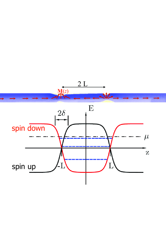
Figure 1: (upper panel) Schematics of the variation of the magnetization $\mathbf{M}$ in a magnetic quantum wire with two domain walls (DWs). The easy plane is chosen as the $x$-$z$ plane. DWs are separated by a distance $2L$. (lower panel) the effective potential profile experienced by spin-up and spin-down electrons. Quasi-localized energy levels are marked by dashed lines. $2\delta$ is the DW width and $\mu$ is the chemical potential.

In this work, we focus on the current and shot noise properties in a particular spin-dependent quantum pump based on two domain walls in a magnetic quantum wire (shown in Fig.1). In general, the transport properties of magnetic domain walls (DWs) are actively discussed and realized for spintronics applications (cf. Ref.Ref24, ; Ref25, ; Ref26, ; Ref27, ; Ref28, and references therein). To our knowledge however, a DW-based quantum pump has not yet been considered. As shown by Dugaev et al.Ref24 in a semiconducting magnetic nanowire, double DWs separated by a distance less than the phase coherence length act as a spin quantum well within which quasistationary spin-dependent quantized states are formed. To generate in this structure a spin-polarized dc current at zero bias voltage we propose to apply a slowly oscillating gate potential and a varying magnetic field. In effect this means a periodic variation of the chemical potential and the scattering strength of the DWs. In the spirit of an adiabatic quantum pump, these varying parameters should oscillate slowly relative to the carriers’ interaction time with the DWs. The DWs themselves however should be sharp and not adiabatic. This renders a strong scattering from DWs and hence the formation of the quantum well. Here we note that conventionally a DW is called adiabatic when its extensions is larger than the Fermi wave length of the carriers Ref26 . Therefore, for an experimental realization low-density magnetic semiconductor based nanowires are favorable, e.g. as reported in Ref.Ref25, . In the following, we investigate the pumping current and shot noise characteristics of this system and explore the pumping properties and the underlying relation between the pump noise and quantum correlation.

II Theoretical formulation

As shown schematically in Fig.(1), we consider a magnetic nanowire with a magnetization profile consisting of two DWs separated by the distance $2L$. The phase coherence length is larger than $2L$. The width of each of the DWs is $2\delta$. The magnetization vector field ${\bf{M}}\left(z\right)$ in both DWs varies within the $x$-$z$ plane with the $z$ axis being along the wire. Thus, $z$ is the easy axis, and the $x$-$z$ plane is the easy plane. As illustrated in Fig.1 we assume further that the magnitude of ${\bf{M}}\left(z\right)$ is hardly changed but its direction, i.e. we can write ${\bf{M}}\left(z\right)=M{\bf{n}}\left(z\right)$, where ${\bf{n}}\left(z\right)$ is a unit vector field. We study the case where the thickness and the width of the wire are small such that only one size-quantized level (i.e. only a single transverse subband) is populated. Such a system is achievable for magnetic semiconductor-based structures with an appropriately tuned carrier density. Adopting a continuum model, we describe the independent carriers motion along the wire coupled to the non-collinear magnetization field ${\bf{M}}(z)$ with a strength determined by the Kondo-type coupling constant $J$. The single-particle Hamiltonian reads then Ref26

$$H=-\frac{{\hbar^{2}}}{{2m}}\frac{{d^{2}}}{{dz^{2}}}-\Theta{{n}}_{z}\left(z\right)\sigma_{z}-\Theta{{n}_{x}}\left(z\right)\sigma_{x},$$ (1)

where $\Theta=JM$ and $n_{x(z)}$ is the $x(z)$ component of ${\bf{n}}\left(z\right)$, and $m$ is the carrier’s effective mass. $\Theta$ is tunable externally, e.g. by a magnetic field. The potential profile is shown in Fig.1. The carriers’ wave functions are expressible as

$$\begin{array}[]{l}\begin{array}[]{*{20}c}{\psi_{k}\left(z\right)=\left[\left({e^{ikz}+Re^{-ikz}}\right)\left|\uparrow\right\rangle+R_{f}e^{\kappa z}\left|\downarrow\right\rangle\right]e^{-iEt/\hbar},}&{z<-L,}\\ \end{array}\\ \begin{array}[]{*{20}c}{\psi_{k}\left(z\right)=\left[\left({Ae^{\kappa z}+Be^{-\kappa z}}\right)\left|\uparrow\right\rangle+\left({Ce^{ikz}+De^{-ikz}}\right)\left|\downarrow\right\rangle\right]e^{-iEt/\hbar},}&{\left|z\right|<L,}\\ \end{array}\\ \begin{array}[]{*{20}c}{\psi_{k}\left(z\right)=\left[Te^{ikz}\left|\uparrow\right\rangle+T_{f}e^{-\kappa z}\left|\downarrow\right\rangle\right]e^{-iEt/\hbar},}&{z>L,}\\ \end{array}\\ \end{array}$$ (2)

where $\left|\uparrow\right\rangle$ ($\left|\downarrow\right\rangle$) is the spin-up (spin-down) component of the carrier states, $k=[2m(E+JM)]^{1/2}/\hbar$, and $\kappa=[2m(JM-E)]^{1/2}/\hbar$. As illustrated in Fig.1, we measure the electron energy $E$ from the midpoint between spin-up and spin-down band edges. The chemical potential $\mu$ is set by the particle density and can be tuned by an external gate $X_{1}$. The non-spin-flip (spin-flip) transmission and reflection coefficients $T$ and $R$ ($T_{f}$ and $R_{f}$) as well as the constants $A$, $B$, $C$, and $D$ can be deduced from the solutions of Eq. (1) and from the wave function continuity requirements. We note, that instead of using the wave function we can equivalently utilize the transmission and reflection amplitudes kidun . For the system depicted in Fig.1 the transmission and the reflection amplitudes $T(\Theta,\mu)$ and $R(\Theta,\mu)$ were derived and given explicitly in Ref.Ref24 (same applies to ($T_{f}$ and $R_{f}$)).

Following the standard scattering approachRef2 ; Ref3 ; Ref29 we introduce the fermionic creation and annihilation operators for the carrier scattering states. The operator $\hat{a}_{L\sigma}^{\dagger}(E)$ or $\hat{a}_{L\sigma}(E)$ creates or annihilates particles with total energy $E$ and spin polarization $\sigma$ in the left lead, which are incident upon the sample. Analogously, we define the creation $\hat{b}_{L\sigma}^{\dagger}(E)$ and annihilation $\hat{b}_{L\sigma}(E)$ operators for the outgoing single-particle states. For magnetic semiconductor nanowires with a moderate carrier density the chemical potential $\mu$ is tunable to be in one of the magnetically split subbands. In this case one achieves a full spin polarization of the electron gas. Therefore, the incident electrons are fully spin polarized. We note that the spin-down part of the wave function decays outside the double-domain-wall (DW) regime (cf. Fig.1). Correspondingly, only spin-up electrons tunnel through the barrier and contribute to the conductance. Furthermore, the energy is conserved during the tunneling process Ref30 . As mentioned above, the wire is such that a single one-dimensional subband is populated and hence the transverse channels are not considered here. The scattering matrix $S$ is follows from the relation

$$\left({\begin{array}[]{*{20}c}{b_{L\uparrow}}\\ {b_{R\uparrow}}\\ \end{array}}\right)=\underbrace{\left({\begin{array}[]{*{20}c}R&{T^{\prime}}\\ T&{R^{\prime}}\\ \end{array}}\right)}_{S}\left({\begin{array}[]{*{20}c}{a_{L\uparrow}}\\ {a_{R\uparrow}}\\ \end{array}}\right),$$ (3)

where, as a result of the structure configuration symmetry the relation $T^{\prime}=T$, $R^{\prime}=R$ appliesRef31 . States that decay exponentially away from the DWs do not contribute directly to the current flow and thus to the scattering matrix. We note that the external magnetic field will be incorporated as an induced change of $\Theta$ in Eq.(1), i.e. as an effective change in the height of DWs.

In the adiabatic regime the external perturbations vary slowly on the scale of the carriers interaction time (Wigner delay time) with the DWs structures. In this case one can employ an instant scattering matrix approach, i.e. $S(t)$ depends only parameterically on the time $t$. To realize a quantum pump one varies simultaneously two system parameters, e.g. Ref2 ; Ref3

$$\begin{array}[]{l}X_{1}\left(t\right)=X_{10}+X_{\omega,1}e^{i\left({\omega t-\varphi_{1}}\right)}+X_{\omega,1}e^{-i\left({\omega t-\varphi_{1}}\right)},\\ X_{2}\left(t\right)=X_{20}+X_{\omega,2}e^{i\left({\omega t-\varphi_{2}}\right)}+X_{\omega,2}e^{-i\left({\omega t-\varphi_{2}}\right)}.\\ \end{array}$$ (4)

Here, $X_{1}$ is a measure for the carrier coupling energy to the DWs (cf. eq.(1)) $\Theta\equiv JM$ which can be modulated by applying a low-frequency ($\omega$) alternating external magnetic field. $X_{2}$ is the Fermi level position $\mu$, which is adiabatically varied by exposing the device to ac gate potential. $X_{\omega,1}$ and $X_{\omega,2}$ are the corresponding oscillating amplitudes with phases $\varphi_{1/2}$; $X_{10}$ and $X_{20}$ are the static (equilibrium) components.

Different from the widely discussed adiabatic spin pump based on an normal metal/ferromagnet/normal metal junction, in our considered system, the direction of the magnetization in the nanowire and DWs remain constant in time: it is along $z$ direction outside the double DW regime and along $-z$ direction between the two DWs; the magnetization of the DWs varies in the $x$-$z$ plane (cf. Fig. 1). Applying an alternating external magnetic field, the strength of the magnetization varies while out-of-plane precession is suppressed by magnetic anisotropy. Hence, effects related to field-induced magnetization precession Ref18 ; Ref19 are not considered here. For the reason that the scattering process has only one spin channel (spin-up channel), the pumped current is spin polarized, as detailed below.

As in the work of Moskalets and Büttiker Ref3 , in the weak pumping limit ($X_{\omega,j}\ll X_{j0}$) and at zero temperature, the spin-polarized pump current, noise, and heat flow could be expressed in terms of the scattering matrix as follows.

$$I_{\alpha}=\frac{{e\omega}}{{2\pi}}\sum\limits_{\beta j_{1}j_{2}}{X_{\omega,j_{1}}X_{\omega,j_{2}}\frac{{\partial S_{\alpha\beta}^{*}}}{{\partial X_{j_{1}}}}\frac{{\partial S_{\alpha\beta}}}{{\partial X_{j_{2}}}}2\sin\left({\varphi_{j_{1}}-\varphi_{j_{2}}}\right)},$$ (5)

$$\hskip 2.84544ptH_{\alpha}=\frac{{\hbar\omega^{2}}}{{4\pi}}\sum\limits_{\beta j_{1}j_{2}}{X_{\omega,j_{1}}X_{\omega,j_{2}}\frac{{\partial S_{\alpha\beta}}}{{\partial X_{j_{1}}}}\frac{{\partial S_{\alpha\beta}^{*}}}{{\partial X_{j_{2}}}}2\cos\left({\varphi_{j_{1}}-\varphi_{j_{2}}}\right)},$$ (6)

$$\begin{array}[]{c}\hskip 11.38092ptS_{\alpha\beta}=\frac{{e^{2}\omega}}{\pi}\left[{\delta_{\alpha\beta}\sum\limits_{\beta j_{1}j_{2}}{X_{\omega,j_{1}}X_{\omega,j_{2}}\frac{{\partial S_{\alpha\beta}}}{{\partial X_{j_{1}}}}\frac{{\partial S_{\alpha\beta}^{*}}}{{\partial X_{j_{2}}}}2\cos\left({\varphi_{j_{1}}-\varphi_{j_{2}}}\right)}}\right.\\ \hskip 85.35826pt\left.{-\sum\limits_{\gamma_{1}j_{1}\gamma_{2}j_{2}}{S_{\beta\gamma_{1}}^{*}S_{\beta\gamma_{2}}X_{\omega,j_{1}}X_{\omega,j_{2}}\frac{{\partial S_{\alpha\gamma_{1}}^{*}}}{{\partial X_{j_{1}}}}\frac{{\partial S_{\alpha\gamma_{2}}}}{{\partial X_{j_{2}}}}2\cos\left({\varphi_{j_{1}}-\varphi_{j_{2}}}\right)}}\right].\\ \end{array}$$ (7)

Here, we remark that capturing the sensitivity of the quantum levels and scattering matrix to general perturbations is a complicated problem entailing the treatment of a time-dependent Hamiltonian. In the limit of an adiabatic pump however, i.e., assuming that the scattering properties follow the time-dependent potentials instantaneously, it is sufficient to expand the time-dependent scattering matrix to first order in the frequency. In addition, the amplitudes $X_{\omega,j}$ are chosen small with respect to their residual values (e.g., the amplitude of $X_{2}$ is smaller than $\Theta$) such that only the terms linear in $X_{\omega,j}$ are relevant in an expansion of the scattering matrix, which leads to a (bi)linear response in the amplitudesRef2 ; Ref3 . The pumped current and the noise relate to the parametric derivatives of the scattering matrix of the systemRef2 ; Ref3 .

For the consideration of the time-reversal symmetry (TRS) in this system we remark the following. The (non-diffusive) scattering region consists of non-collinear localized magnetic moments (that build the DWs) which reverse sign upon time-reversal. This operation leads in general to different scattering and pump properties trs . In our particular case however, upon time-reversal, the spin polarizations of the states left and right to the DWs is reversed and outgoing waves turn into incoming waves and vice versa. In total, even though the individual wave functions and the scattering region are modified upon a time-reversal, we observe no physical effect of this operation. The situation would be different, if for example the wire to the right side of the DWs were paramagnetic. An elaboration on this point is given below.

Here, we start by specifying the single particle states and calculate with those the T matrices. The time-reversal of the carrier wave functions (2) can be obtained as

$$\begin{array}[]{l}\begin{array}[]{*{20}c}{\psi_{k}\left(z\right)=\left[\left({e^{-ikz}+R^{*}e^{ikz}}\right)\left|\downarrow\right\rangle+R_{f}^{*}e^{\kappa z}\left|\uparrow\right\rangle\right]e^{iEt},}&{z<-L,}\\ \end{array}\\ \begin{array}[]{*{20}c}{\psi_{k}\left(z\right)=\left[\left({A^{*}e^{\kappa z}+B^{*}e^{-\kappa z}}\right)\left|\downarrow\right\rangle+\left({C^{*}e^{-ikz}+D^{*}e^{ikz}}\right)\left|\uparrow\right\rangle\right]e^{iEt},}&{\left|z\right|<L,}\\ \end{array}\\ \begin{array}[]{*{20}c}{\psi_{k}\left(z\right)=\left[T^{*}e^{-ikz}\left|\downarrow\right\rangle+T_{f}^{*}e^{-\kappa z}\left|\uparrow\right\rangle\right]e^{iEt},}&{z>L.}\\ \end{array}\\ \end{array}$$ (8)

Spin-up electrons tunnel through the double-domain-wall structure by spin-flip-assisted transmission. When the time is reversed, the angular momentum of the electrons, here the spin, is reversed. As time flows backwards, spin-down electrons tunnel backward through the double-domain-wall structure by spin-flip-assisted transmission. The time-reversed scattering matrix is the Hermitian conjugate of the original one with the transmission probability exactly identical. The nature of DWs is that of an angular momentum. Time reversal reverses the sign of the localized moments, forming thus an anti-double-domain-wall structure with a spin-down well between the two domain walls. Outside the domain wall structure, the time-reversed magnetic nanowire favors then a transport of spin-down electrons. In the adiabatic limit, the applied external magnetic field is effectively incorporated in the behavior of the DWs. Or it is equivalent to say that the effect of the time-reversal transformation reverses the direction of the magnetic field and that reverses the magnetic configuration. To contrast this situation with what is established in the literature we recall that in Ref.[Ref2, ] Brouwer considered a chaotic quantum dot with the conclusion that the distribution of the pumped current for systems with TRS and those without TRS are remarkably different. In our consideration the strength of the particle flow is conserved through tunneling, which is required by the continuity equation for the Schrödinger equation. The time reversed tunneling would generate exactly the same pumped current with the electron spin reversed. In our case, the distribution of the pumped current is not a defined quantity or is a constant.

Under the assumption that the scattering properties follow the time-dependent potentials instantaneously, calculating the parametric derivative of the scattering matrix is a numerical issue as demonstrated in the literatureRef3 ; Ref4 including Brouwer’s seminal approachRef2 . In our work, the stationary transmission and reflection coefficients were analytical obtained along with their parametric derivatives. The derivative of the scattering matrix can be inferred from the stationary Hamiltonian: an infinitesimal change in the external parameters (here, the magnetization field and the Fermi energy) alters the Hamiltonian and hence the scattering matrix. Accordingly, in the adiabatic limit, we can find the derivative without introducing a time-dependent Hamiltonian. In the linear response situation, all the sensitivity of the scattering matrix to the perturbations lies in its parametric derivatives.

Considering an adiabatic pump, the modulation frequency $\omega$ is assumed to be extremely small relative to the interaction time of the system. The current and noise vary linearly with $\omega$, which is within the theory of an adiabatic pumpRef3 and demonstrated in experimentRef1 . The first term in Eq. (7) reflects the strength of the energy flow while the second one describes the effect of correlations between (quasi)-particles. A convenient measure of the correlation is $F=\frac{{\hbar\omega}}{{4e^{2}}}\frac{S_{\alpha\beta}}{H_{\alpha}}$, which is the ratio of the dimensionless strength of the shot noise $S_{\alpha\beta}$ and the heat flow. The pump current and the noise experience sinusoidal and cosinusoidal variations as functions of the phase difference $\Delta\varphi=\varphi_{1}-\varphi_{2}$ respectively, as is evident in Eqs. (5) and (7). The relative noise $F$ does not vary with $\Delta\varphi$.

III Numerical results and interpretations

In a magnetic nanowire with double sharp magnetic DWs, quantum interference results in the formation of spin-split quasistationary states localized mainly between the domain wallsRef24 . Consequently, the DWs conductance exhibits typical resonant tunneling behaviour. The width of the resonance peaks is related to $\tau$, the lifetime of the quasistationary spin quantum well states. $\tau$ is determined by the spin-mixing due to the spin noncollinearity at the DWs and can be quantified by the spin-mixing parameter $\Delta\equiv 4m\Theta\delta/\hbar^{2}$. Decreasing $\Delta$, the lifetime of the localized spin quantum-well states increases and the conductance resonance peaks become correspondingly narrower. By oscillating the gate potential and the magnetic field strength out of phase at zero bias, a quantum pump is realized as the electronic system gains energy from the oscillating scatterer. Absorption of an energy quantum $\hbar\omega$ leads to creation of a nonequilibrium quasi-electron-hole pair. If they are scattered into different leads, their motion generates current.

In the adiabatic quantum pump based on domain walls in a magnetic nanowire considered here, the two parameters are the Fermi energy and the magnetization strength, which excite the pump. The Fermi energy can be modulated by an ac gate voltage and the magnetization strength can be modulated by an ac magnetic field. Analogously to the adiabatic quantum electron pump theoretically proposed in Ref. Ref2, and experimentally realized in the quantum dot systemRef1 , in our case the oscillating magnetization acts as an oscillating energy potential (cf. Fig.1). The two oscillating parameters we view as two out-of-phase gating potentials, one from the ac electric modulation, and the other from the ac magnetic modulation; on the other hand the quantum dot pump system experiences two oscillating gates. Electrons absorb or emit an energy quantum from the oscillating mesoscopic scatterer and those pumped to different directions contribute to the current. The external electric gate voltage oscillating at the spin-split quasistationary states excites pumping current and gives rise to the resonance-type peaks in the current. Within the two-gate picture, the DW quantum pump system can be viewed semiclassically as in the turnstile quantum dot—a classical analog of quantum pumpingRef32 .

Fig. 2 shows the tunneling current without external modulations as well as the current adiabatically pumped by the modulations (4) as functions of the Fermi energy. In Fig. 2 (b), the phase difference $\Delta\varphi$ is set to be $-\pi/2$ to produce maximal pump current and to demonstrate the pumping properties prominently. The conductance of the double DW structure possesses sharp resonances when the Fermi energy matches the spin quantum-well states as seen in Fig 2 (a) and Ref.Ref24, . Similarly, in the circumstance of the adiabatic pump, the electron can only tunnel through the spin-split levels between the two domains. Thus, the pump current, shot noise and heat flow show peak structures when the Fermi energy matches the spin quantum-well states (see also Fig. 3).

Comparing panels (a) and (b) in Fig. 2 we find that the peak height (PH) of the pumped current decreases dramatically as the width of the DWs is increased. For narrower DWs, the peak width (PW) of the pumped current becomes more comparable with that of the linear-response conductance, while for wider DWs the former is much smaller than the latter. To further reveal the trend, the PH and the PW at half peak height of the pumped current versus $\delta$ are given in Figs. 4 and 5 respectively for the second quasistationary level counting from the spin quantum-well bottom. The peak height decreases exponentially with the increase of $\delta$. In contrast to the linear-response process, the pumping process depends strongly on the lifetime of the quasistationary, spin-well states. When the period of the pump $\tau_{p}=2\pi/\omega$ exceeds the lifetime of the quasistationary states, the pumped current would be greatly suppressed. Here, we consider the limit of small modulation frequencies, i.e. an adiabatic pumpRef3 meaning that $\tau_{p}$ is relatively large. Therefore, the strength of the pumped current decreases exponentially with the widening of the DW, i.e., the decrease of the lifetime of the quasistationary states.

In the adiabatic limit, i.e. when the frequency of the potential modulation is small compared to the characteristic times for traversal and reflection of electrons, the photon side band $E_{F}\approx E_{r}\pm\hbar\omega$ broadens the current peak instead of forming new peaks as in Ref.Ref5, . In principle, without the external modulations the resonant tunnelling current is broadened due to spin mixing at the DWs. If the spin-mixing amplitude is finite (i.e., $\Delta\neq 0$), spin-up carriers transverse resonantly the DWs and the conductance peaks are broadened by the spin-mixing mechanism. For very narrow DWs the residual broadening can then be attributed to the side-band formation.

In the theory of an adiabatic quantum pump, the nearest sidebands corresponding to particles which have gained or lost a modulation quantum $\hbar\omega$ contribute to the pumped current. Hence, the pumped current peak is broadened by $2\hbar\omega$ at the resonant levels. The width of peaks in the linear-response conductance due to spin mixing at the DWs is enhanced for wider DWs (cf. Fig. 5). In comparison, the broadening of the pumped current peaks caused by the sideband formation is less pronounced for varying DW extensions. For very sharp DWs however the effect of the side-band formations might be as large as the contribution from the DWs spin mixing.

To demonstrate the quantum pump noise properties in this particular structure, we present the numerically obtained pump current $I$, shot noise $S$, heat flow $H$, and relative pump noise $F$ as functions of the Fermi energy in Fig. 3. The properties for different DW distance $L$ are compared. The pump current, shot noise and heat flow show peak structure when the Fermi energy matches with the resonant energy levels of the structure. The peak position changes accordingly as the resonant levels shift to lower energy when we increase the DW distance $L$. The ratio between the pump shot noise and the heat flow $F$ reflects the strength of the quantum correlation of the system. $F$ shows bifurcated peaks with the intermediate minima at the resonant Fermi energies.

The pump noise properties can be interpreted as follows. At the resonant Fermi energy, transport processes and thus the electron-electron correlation achieve maximal strength. The nonequilibrium quasi-electrons and holes created by the oscillating scatterer move in different directions to generate a net dc current. Therefore, the antibunching correlation between electrons and holes always exerts a negative contribution to the shot noise regardless of the direction of the dc current, which gives rise to the minimum valley in the relative noise. At the edges of the resonant state, there is a slight heat flow in the dissipation regime without actual particle motion. In this region, the heat flow dominates the quasiparticle correlation giving rise to full heat flow noise with $F=1$. In the intervals between resonant levels, heat flow and quasiparticle correlation both approach a background level inducing zero pump shot noise.

IV Conclusions

In summary, a quantum pump device involving domain walls in a magnetic nanowire is investigated. For two independent adiabatically modulated parameters of this device a finite net charge current is transported. The quantum pumping mechanism resembles the quantum pump based on two-oscillating-gate quantum dot and is to some extent analogous to the classical turnstile picture. The pumping current, heat flow, and shot noise demonstrate peak structures at the spin-split quasistationary levels in the spin-quantum well formed by the domain walls. The strength of the pump current decreases exponentially with the decrease of the quasistationary-state lifetime. The latter is governed by the width of the domain wall. The sideband formation during the pumping process is sizable particularly for narrow domain wall for which level broadening due to spin-mixing is relatively small. The correlation between quasielectrons and quasiholes shows antibunching behavior as they move in opposite directions. This is concluded from the ratio between the pump shot noise and the heat flow.

Figure 2: Linear-response conductance (a) and pump current $I$ (b) as functions of the Fermi energy $E_{F}$ for different DW width $\delta$. The parameters are chosen as follows: The coupling of the carriers to the DWs is $\Theta\equiv JM=2.4$ meV; the amplitudes of the external perturbations are $\Theta_{\omega}=X_{1,\omega}=0.1$ meV $=\mu_{\omega}=X_{2,\omega}$; the distance between the DWs is $L=15$ nm. In panel (b), the parameters are set in the weak pumping regime.

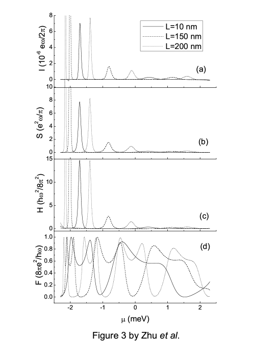
Figure 3: Pump current $I$ (a), pump noise $S$ (b), heat flow $H$ (c), and relative noise $F$ (d) as functions of the Fermi energy $E_{F}$ for different DW distance $L$. DWs width is $\delta=2$ nm and the other parameters are the same to Fig. 1 (b).

Figure 4: The peak height (PH) of the pumped current as a function of the DW width $\delta$ for the second quasistationary level counting from the spin well bottom. The parameters are the same to Fig. 1 (b).

Figure 5: The peak width (PW) at half peak height of the linear-response conductance (dot) and the pumped current (square) respectively as a function of the DW width $\delta$ for the second quasistationary level counting from the spin well bottom. The parameters are the same to Fig. 1 (b).

References

- (1) M. Switkes, C. M. Marcus, K. Campman, and A. C. Gossard, Science 283, 1905 (1999).
- (2) P. W. Brouwer, Phys. Rev. B 58, R10135 (1998). M. Büttiker, H. Thomas, and A. Prêtre, Z. Phys. B 94, 133 (1994); Phys. Rev. Lett. 70, 4114 (1993).
- (3) M. Moskalets and M. Büttiker, Phys. Rev. B 66, 035306 (2002).
- (4) R. Benjamin and C. Benjamin, Phys. Rev. B 69, 085318 (2004).
- (5) H. C. Park and K. H. Ahn, Phys. Rev. Lett. 101, 116804 (2008).
- (6) P. Devillard, V. Gasparian, and T. Martin, Phys. Rev. B 78, 085130 (2008).
- (7) R. Citro and F. Romeo, Phys. Rev. B 73, 233304 (2006).
- (8) M. Moskalets and M. Büttiker, Phys. Rev. B 72, 035324 (2005).
- (9) M. Moskalets and M. Büttiker, Phys. Rev. B 75, 035315 (2007).
- (10) F. Romeoa and R. Citro, Eur. Phys. J. B 50, 483 (2006).
- (11) J. Splettstoesser, M. Governale and J. König, Phys. Rev. B 77, 195320 (2008).
- (12) M. Strass, P. Hänggi, and S. Kohler, Phys. Rev. Lett. 95, 130601 (2005).
- (13) J.E. Avron, A. Elgart, G.M. Graf, and L. Sadun, Phys. Rev. Lett. 87, 236601 (2001).
- (14) B. G. Wang, J. Wang, and H. Guo, Phys. Rev. B 65, 073306 (2002).
- (15) B. G. Wang and J. Wang, Phys. Rev. B. 66, 125310 (2002).
- (16) B. G. Wang, J. Wang, and H. Guo, Phys. Rev. B 68, 155326 (2003).
- (17) L. Arrachea, Phys. Rev. B 72, 125349 (2005).
- (18) Y. Tserkovnyak, A. Brataas, G. E. W. Bauer, and B. I. Halperin, Rev. Mod. Phys. 77, 1375 (2005).
- (19) D. C. Ralph and M. D. Stiles, J. Magn. Magn. Mater. 320, 1190 (2008).
- (20) Y.M. Blanter and M. Büttiker, Physics Reports 336, 1 (2000).
- (21) M. Büttiker, Phys. Rev. Lett. 65, 2901 (1990).
- (22) R. Zhu and Y. Guo, Appl. Phys. Lett. 90, 232104 (2007).
- (23) J. C. Egues, G. Burkard, D. S. Saraga, J. Schliemann, and D. Loss, Phys. Rev. B 72, 235326 (2005).
- (24) V. K. Dugaev, J. Berakdar, and J. Barnaś, Phys. Rev. Lett. 96, 047208 (2006).
- (25) C. Rüster, T. Borzenko, C. Gould, G. Schmidt, L. W. Molenkamp, X. Liu, T. J. Wojtowicz, J. K. Furdyna, Z. G. Yu, and M. E. Flatté, Phys. Rev. Lett. 91, 216602 (2003).
- (26) V. K. Dugaev, J. Berakdar, and J. Barnaś, Phys. Rev. B 68, 104434 (2003); V. K. Dugaev, J. Barnaś, J. Berakdar, V. I. Ivanov, W. Dobrowolski, and V. F. Mitin, Phys. Rev. B 71, 024430 (2005); V. K. Dugaev, J. Barnaś, and J. Berakdar, J. Phys. A 36, 9263 (2003).
- (27) G. A. Prinz, Science 282, 1660 (1998); S. A. Wolf, D. D. Awschalom, R. A. Buhrman, J. M. Daughton, S. von Molnr, M. L. Roukes, A. Y. Chtchelkanova, and D. M. Treger, Science 294, 1488 (2001).
- (28) A. Yamaguchi, T. Ono, S. Nasu, K. Miyake, K. Mibu, T. Shinjo, Phys. Rev. Lett. 92, 077205 (2004); M. Yamanouchi, D. Chiba, F. Matsukura, and H. Ohno, Nature (London) 428, 539 (2004); E. Saltoh, H. Miyajima, T. Yamaoka, and G. Tatara, Nature (London) 432, 203 (2004).
- (29) O. Kidun, N. Fominykh, J. Berakdar Phys. Rev. A 71, 022703/1 (2005).
- (30) D. K. Ferry and S. M. Goodnick, in Transport in Nanostructures, (Cambridge University Press, 1997).
- (31) When the pumping mechanism is taken into account, the scattering matrix elements vary with the oscillating parameters. A scattered electron can absorb or emit one energy quantum before it leaves the scattering region. This does not contradict our single-channel picture.
- (32) In most quantum transport problems the transmission coefficients seen from the two sides of the scattering region differ at least in phase. Structural configuration symmetry imposes however the relations and . The structure of the double-DW nanowire system is symmetric. The band edge does not vary in the transmission direction, which means that the band profile seen from the left is exactly the same with that seen from the right (cf. Fig.1). Having derived analytically and from spatially inverted wave functions we confirmed explicitly the above statement.
- (33) M. L. Polianski, M. G. Vavilov, and P. W. Brouwer, Phys. Rev. B 65, 245314 (2002).
- (34) L. P. Kouwenhoven, A. T. Johnson, N. C. van der Vaart, C. J. P. M. Harmans, and C. T. Foxon, Phys. Rev. Lett. 67, 1626 (1991).