${\cal N}=1$ Wess Zumino Model in $d=3$ at zero and finite temperature

Abstract

Supersymmetric renormalization group (RG) flow equations for the effective superpotential of the three-dimensional Wess-Zumino model are derived at zero and non-zero temperature. This model with fermions and bosons interacting via a Yukawa term possesses a supersymmetric analogue of the Wilson-Fisher fixed-point. At zero temperature we determine the phase-transition line in coupling-constant space separating the supersymmetric from the nonsupersymmetric phase. At finite temperature we encounter dimensional reduction from $3$ to $2$ dimensions in the infrared regime. We determine the finite-temperature phase diagram for the restoration of the global $\mathbbm{Z}_{2}$-symmetry and show that for temperatures above the $\mathbbm{Z}_{2}$ phase-transition the pressure obeys the Stefan-Boltzmann law of a gas of massless bosons in $2+1$ dimensions.

I Introduction

In this paper we investigate the three-dimensional $\mathcal{N}=1$ Wess-Zumino model with general superpotential and explore the model beyond the realm of perturbative expansions. This quantum field theory describes Majorana fermions and uncharged bosons in interaction, with their spatial motion restricted to a two-dimensional layer. The selfcoupling of the bosons and the Yukawa coupling between fermions and bosons are such that the theory possesses one supersymmetry. There exists a class of superpotentials for which the three-dimensional models are perturbatively renormalizable, in contrast to the four-dimensional models. For superpotentials of the form $W(\phi)\sim\lambda\phi^{2n+1}$ there exists both a supersymmetric and a nonsupersymmetric phase. In this paper we shall calculate the phase-transition curve separating the supersymmetric from the nonsupersymmetric phase. Besides supersymmetry the action is invariant under $\phi\to-\phi$, and at zero temperature the breaking of this global ${\mathbb{Z}}_{2}$ symmetry is intimately linked to the breaking of supersymmetry. We shall see that there exists a finite phase-transition temperature at which ${\mathbb{Z}}_{2}$ symmetry is restored, independent of our choice for the couplings at the cutoff-scale. Similarly as for other two-dimensional systems, e.g. surface science, heterostructures or electron gases, the physics in two space-dimensions is rather different from that in three space-dimensions.

We employ the functional renormalization group (RG) to calculate the phase structure at zero and finite temperature, the scaling behavior of the mass with the RG-scale, the wave-function renormalization, critical exponents, the effective potential and the temperature dependence of the pressure. The method has previously been applied to a wide range of nonperturbative problems such as critical phenomena, fermionic systems, gauge theories and quantum gravity, see Litim:1998nf ; Aoki:2000wm ; Berges:2000ew ; Polonyi:2001se ; Pawlowski:2005xe ; Gies:2006wv ; Sonoda:2007av ; Delamotte:2007pf for reviews. A number of conceptual studies of supersymmetric theories has already been performed with the functional RG. The delicate point here is, of course, the construction and use of a manifestly supersymmetry-preserving regulator. For the four-dimensional Wess-Zumino model such a regulator has been presented in Vian:1998kv ; Bonini:1998ec . Recently, general theories of a scalar superfield including the Wess-Zumino model have been investigated with a Polchinski-type RG equation in Rosten:2008ih , yielding a new approach to supersymmetric nonrenormalization theorems. A Wilsonian effective action for the Wess-Zumino model by perturbatively iterating the functional RG has been constructed in Sonoda:2008dz .

The present study builds on our earlier results on two-dimensional supersymmetric field theories at zero temperature Synatschke:2009nm ; Gies:2009az as well as on supersymmetric quantum mechanics, where we have constructed a manifestly supersymmetric functional RG flow, see Synatschke:2008pv . The two-dimensional models possess an infinite series of fixed points described by two-dimensional super-conformal theories. On the contrary, supersymmetric models in three dimensions possess just one fixed point, similarly as three-dimensional $O(N)$ models, see e. g. Berges:2000ew ; Tetradis:1993ts ; Litim:2002cf ; Bervillier:2007rc .

In the present work we first sketch the derivation of the manifestly supersymmetric flow equations in Sect. III. Since there exist no Majorana fermions in three-dimensional Euclidean spacetime we derive the flow equations in Minkowski spacetime and continue the result to imaginary time. We investigate the flow of the superpotential in Sect. III.1, study the fixed-point structure in detail, and identify the supersymmetric analogue of the Wilson-Fisher fixed point of three-dimensional bosonic $O(N)$ models with one unstable direction. Taking into account a nonzero anomalous dimension in Sect. III.2 yields a scaling relation between the critical exponent of the unstable direction and the anomalous dimension. In addition we determine the zero-temperature phase diagram for spontaneous breaking of supersymmetry.

The second part of this paper is devoted to the behavior of the model at finite temperature. The fate of supersymmetry at finite temperature has been discussed extensively in the literature. For example, in previous works the KMS condition has been implemented directly in thermal superspace Derendinger:1998zj . In Das:1978rx ; Girardello:1980vv the supersymmetry breaking has been studied on the level of thermal Green functions. The breaking of supersymmetry by finite temperature corrections, for example the one-loop corrections to fermionic and bosonic masses, has been determined in the real-time formulation in Midorikawa:1984fi . The inevitable breaking of supersymmetry at finite temperature has sometimes been called spontaneous collapse of supersymmetry Buchholz:1997mf .

In Sect. IV we derive the RG flow equations at finite temperature. In addition to the momentum integrals we are confronted with sums over Matsubara frequencies. For the three-dimensional Wess-Zumino model and for a particular regulator the thermal sums can be calculated analytically. Related sums have been discussed in earlier works on finite-temperature renormalization group flow equations, for example in Litim:2000ci ; Litim:2001up ; Braun:2006jd ; Litim:2006ag ; Blaizot:2006rj ; Floerchinger:2008qc ; Braun:2009si ; Diehl:2009ma . We observe that the Wess-Zumino model in three dimensions at finite temperature in the $\mathbbm{Z}_{2}$ symmetric phase behaves similarly to a gas of massless bosons. In particular we show in Sect. IV.1 that it obeys the Stefan-Boltzmann law in three dimensions. For high temperatures the fermions do not contribute to the flow equations since they do not have a thermal zero-mode. On the other hand we observe dimensional reduction in the bosonic part of the model due to the presence of a thermal zero-mode. We show in Sect. IV.2 how this is manifested in our RG framework. In a similar way dimensional reduction has been observed in $O(N)$-models at finite temperature in Tetradis:1992xd ; Bohr:2000gp . Finally we compute the phase diagram for the restoration of the global $\mathbb{Z}_{2}$ symmetry at finite temperature in Sect. IV.3.

II The $\mathcal{N}=1$ Wess-Zumino model in three dimensions at $T=0$

There are many works on the supersymmetric Wess-Zumino models in both four and two space-time dimensions. Actually the two-dimensional model with $\mathcal{N}=2$ supersymmetries is just the toroidal compactification of the four-dimensional $\mathcal{N}=1$ model. The three-dimensional model with $\mathcal{N}=1$ supersymmetry, on the other hand, cannot be obtained by dimensional reduction of a local field theory in four dimensions. Thus it may be useful to recall the construction of the three-dimensional model starting from the real superfield

$$\Phi(x,\alpha)=\phi(x)+\bar{\alpha}\psi(x)+\frac{1}{2}\bar{\alpha}\alpha F(x)$$ (1)

with real (pseudo)scalar fields $\phi,F$ and Majorana spinorfield $\psi$. The supersymmetry variations are generated by the supercharge

$$\delta_{\beta}\Phi=i\bar{\beta}\mathcal{Q}\Phi,\quad\mathcal{Q}=-i\frac{\partial}{\partial\bar{\alpha}}-(\gamma^{\mu}\alpha)\partial_{\mu}\,.$$ (2)

We use the metric tensor $(\eta_{\mu\nu})=\hbox{diag}(1,-1-1)$ to lower Lorentz indices. With the aid of the symmetry relations for Majorana spinors $\bar{\psi}\chi=\bar{\chi}\psi,\;\bar{\psi}\gamma^{\mu}\chi=-\bar{\chi}\gamma^{\mu}\psi$ and the particular Fierz identity $\alpha\bar{\alpha}=-\bar{\alpha}\alpha\,\mathbbm{1}/2$ the transformation laws for the component fields follow from Eq. (2):

$$\delta\phi=\bar{\beta}\psi,\quad\delta\psi=(F+i\not{\partial}\phi)\beta,\quad\delta F=i\bar{\beta}\not{\partial}\psi\,.$$ (3)

The anticommutator of two supercharges yields $\left\{\mathcal{Q}_{\alpha},\bar{\mathcal{Q}}^{\beta}\right\}=2{(\gamma^{\mu})_{\alpha}}^{\beta}\partial_{\mu}$. The supercovariant derivatives are

$$\mathcal{D}=\frac{\partial}{\partial\bar{\alpha}}+i(\gamma^{\mu}\alpha)\partial_{\mu},\quad\text{and}\quad\bar{\mathcal{D}}=-\frac{\partial}{\partial\alpha}-i(\bar{\alpha}\gamma^{\mu})\partial_{\mu}.$$ (4)

Up to a sign they obey the same anticommutation relation as the supercharges

$$\{\mathcal{D}_{\alpha},\bar{\mathcal{D}}^{\beta}\}=-2{(\gamma)_{\alpha}}^{\beta}\partial_{\mu}\,.$$ (5)

As kinetic term we choose the $D$ term of $\bar{\mathcal{D}}\Phi\mathcal{D}\Phi=2\bar{\alpha}\alpha\mathcal{L}_{\rm kin}+\dots$ which reads

$$\mathcal{L}_{\rm kin}=\frac{1}{2}\partial_{\mu}\phi\partial^{\mu}\phi-\frac{i}{2}\bar{\psi}\not{\partial}\psi+\frac{1}{2}F^{2}.$$ (6)

The interaction term is the $D$ term of $2W(\Phi)=\bar{\alpha}\alpha\mathcal{L}_{\rm int}+\dots$ and contains a Yukawa term,

$$\mathcal{L}_{\rm int}=FW^{\prime}(\phi)-\frac{1}{2}W^{\prime\prime}(\phi)\bar{\psi}\psi.$$ (7)

The complete off-shell Lagrange density $\mathcal{L}_{\rm off}=\mathcal{L}_{\rm kin}+\mathcal{L}_{\rm int}$ takes then the simple form

$$\mathcal{L}_{\rm off}=\frac{1}{2}\partial_{\mu}\phi\partial^{\mu}\phi-\frac{i}{2}\bar{\psi}\not{\partial}\psi+\frac{1}{2}F^{2}+FW^{\prime}(\phi)-\frac{1}{2}W^{\prime\prime}(\phi)\bar{\psi}\psi.$$ (8)

Eliminating the auxiliary field via its equation of motion $F=-W^{\prime}(\phi)$, we end up with the on-shell density

$$\mathcal{L}_{\rm on} =\frac{1}{2}\partial_{\mu}\phi\partial^{\mu}\phi-\frac{i}{2}\bar{\psi}\not{\partial}\psi-\frac{1}{2}W^{\prime 2}(\phi)-\frac{1}{2}W^{\prime\prime}(\phi)\bar{\psi}\psi.$$ (9)

From this expression we read off that $W^{\prime 2}(\phi)$ acts as a self-interaction potential for the scalar fields. For a polynomial superpotential $W(\phi)$ in which the power of the leading term is even, $W(\phi)=c\phi^{2n}+\mathcal{O}(\phi^{2n})$, we do not observe supersymmetry breaking in our present non-perturbative renormalization group study. On the other hand spontaneous supersymmetry breaking is definitely possible for a superpotential in which the power of the leading term is odd. In the explicit calculations we shall use a Majorana representation for the $\gamma$-matrices, $\gamma^{0}=\sigma_{2},\,\gamma^{1}=i\sigma_{3}$ and $\gamma^{2}=i\sigma_{1}.$

III Flow equation at zero temperature

To find a manifestly supersymmetric flow equation in the off-shell formulation we extend our earlier results on the one- and two-dimensional Wess-Zumino models Synatschke:2009nm ; Synatschke:2008pv to three dimensions. Since there are no Majorana fermions in three-dimensional Euclidean space we begin with a Minkowski spacetime formulation of the Wetterich equation Wetterich:1992yh ; Berges:2008sr :

$$\partial_{t}\Gamma_{k}=\frac{i}{2}\mathrm{Str}\left[\left(\Gamma_{k}^{(2)}+R_{k}\right)^{-1}\partial_{t}R_{k}\right],\quad t=\ln k^{2}\,,$$ (10)

where the scale-dependent effective action $\Gamma_{k}$ interpolates between the microscopic (classical) action $\Gamma_{k=\Lambda}=S$ and the full quantum effective action $\Gamma_{k=0}=\Gamma$. The second functional derivative in Eq. (10) is defined as

$$\left(\Gamma_{k}^{(2)}\right)_{ab}=\frac{\overrightarrow{\delta}}{\delta\Psi_{a}}\Gamma_{k}\frac{\overleftarrow{\delta}}{\delta\Psi_{b}}\,,$$

where the indices $a,b$ denote the field components, internal and Lorentz indices, as well as space-time or momentum coordinates, i.e., $\Psi^{\text{T}}=(\phi,F,\psi,\bar{\psi})$ is a vector of fields, not to be confused with a superfield. The cutoff function $R_{k}$ provides an infrared (IR) cut-off for all fields and specifies the Wilsonian momentum-shell integrations such that the flow of $\Gamma_{k}$ is dominated by modes $p^{2}\simeq k^{2}$. For a derivation of the RG flow equation in Minkowski space-time (10) we refer to App. A.

To construct a supersymmetric flow we use as regulator an invariant $D$ term in superspace. Since such a term should be quadratic in the fields, see App. A for details, it is the $D$ term of a superfield $\Phi K\Phi$ with $K$ being a function of $\bar{\mathcal{D}}\mathcal{D}$. Using the anticommutation relation (5), powers of $\bar{\mathcal{D}}\mathcal{D}$ can always be decomposed into

$$\Big{(}\frac{1}{2}\bar{\mathcal{D}}\mathcal{D}\Big{)}^{2n}=(-\Box)^{n}\,,$$ (11)

such that an invariant and quadratic regulator action is the superspace integral of

$$\Phi K(\bar{\mathcal{D}}\mathcal{D})\Phi=\Phi\left(r_{1}(-\Box)-r_{2}(-\Box)\frac{\bar{\mathcal{D}}\mathcal{D}}{2}\right)\Phi.$$ (12)

Expressed in component fields, we find

$$\Delta S_{k}=\frac{1}{2}\int(\phi,F)R^{\rm B}_{k}\,{\phi\choose F}+\frac{1}{2}\int\bar{\psi}R^{\rm F}_{k}\psi.$$ (13)

In momentum space, $i\partial_{\mu}$ is replaced by $p_{\mu}$ and the operators take the explicit forms

$$R_{k}=\begin{pmatrix}R_{k}^{\rm B}&0\\ 0&R_{k}^{\rm F}\end{pmatrix}$$ (14)

with

$$R_{k}^{\rm B}=\begin{pmatrix}p^{2}r_{2}&r_{1}\\ r_{1}&r_{2}\end{pmatrix},\quad\text{and}\quad R_{k}^{\rm F}=-r_{1}-r_{2}\not{p}\,,$$ (15)

where $r_{1}=r_{1}(p^{2}/k^{2})$ and $r_{2}=r_{2}(p^{2}/k^{2})$. Note that the requirement that the RG flow preserves supersymmetry relates the regulators $R^{\rm B}_{k}$ and $R^{\rm F}_{k}$ in the bosonic and fermionic subsectors.

III.1 Local Potential Approximation

We employ the following ansatz for the supersymmetric effective action for our study of the three-dimensional Wess-Zumino model:

$$\begin{split}\Gamma_{k}=\int d^{3}x\left[\frac{1}{2}\partial_{\mu}\phi\partial^{\mu}\phi-\frac{i}{2}\bar{\psi}\not{\partial}\psi+\frac{1}{2}F^{2}\right.\\ \left.+FW_{k}^{\prime}(\phi)-\frac{1}{2}W_{k}^{\prime\prime}(\phi)\bar{\psi}\psi\right].\end{split}$$ (16)

In the following we work in the so-called local potential approximation (LPA) where the expectation values of the fields are taken to be constant over the entire volume. As it has been found in studies of scalar $O(N)$ models and low-energy QCD models, the LPA captures already most qualitative and quantitative features associated with critical dynamics at zero and finite temperature provided the anomalous dimensions are small, see e. g. Refs Tetradis:1993ts ; Berges:2000ew ; Bohr:2000gp ; Litim:2002cf ; Bervillier:2007rc ; Braun:2009si . For the time being we restrict our study to LPA. In Sect. III.2 we shall then discuss the running of the wave-function renormalization.

In order to obtain a flow equation for the superpotential, we project Eq. (10) onto the terms linear in the auxiliary field $F$ and integrate the resulting $W^{\prime}_{k}$ with respect to $\phi$. Performing a Wick rotation of the zeroth component of the momentum, i. e. $p_{0}^{M}\to ip_{0}^{E}$, we find the flow equation

$$\partial_{k}W_{k}(\phi)=\frac{1}{2}\int\frac{d^{3}p}{(2\pi)^{3}}\frac{\partial_{k}r_{1}(1+r_{2})-\partial_{k}r_{2}(W^{\prime\prime}_{k}(\phi)-r_{1})}{p^{2}(r_{2}+1)^{2}+(W^{\prime\prime}_{k}(\phi)+r_{1})^{2}}\,.$$ (17)

In the following we choose the simple regulator functions

$$r_{1}=0,\quad r_{2}=\left({\frac{k}{|p|}}-1\right)\theta(k^{2}-p^{2}),$$ (18)

for which the momentum integration in (17) can be performed analytically. In the present work we do not aim at a study the regulator dependence. However, the regulator dependence of functional RG flows, in particular with respect to critical phenomena, has been investigated in great detail and it has been shown that optimized regulator functions minimizing the trucational error can be constructed, see e. g. Refs. Litim:2000ci ; Litim:2001up ; Litim:2001hk ; Litim:2002cf ; Pawlowski:2005xe ; Litim:2006ag .

Contrary to the model in two dimensions Synatschke:2009nm , the regulator function (18) regularizes the flow even if we allow for running wave function renormalizations. For the superpotential $W_{k}$ we then obtain the simple flow equation

$$\partial_{k}W_{k}=-\frac{k^{2}}{8\pi^{2}}\frac{W^{\prime\prime}_{k}(\phi)}{k^{2}+W^{\prime\prime}_{k}(\phi)^{2}}.$$ (19)

As we are interested in the bosonic potential $V(\phi)=W^{\prime 2}(\phi)/2$ we will consider mostly the flow equation for $W^{\prime}_{k}(\phi)$ which reads

$$\partial_{k}W_{k}^{\prime}=-\frac{k^{2}W_{k}^{(3)}(\phi)\left(k^{2}-W_{k}^{\prime\prime}(\phi)^{2}\right)}{8\pi^{2}\left(k^{2}+W_{k}^{\prime\prime}(\phi)^{2}\right)^{2}}.$$ (20)

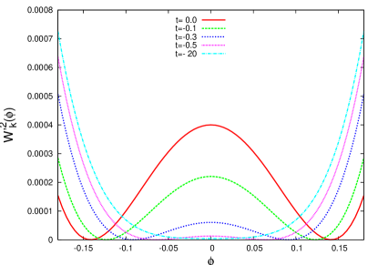
Figure 1: RG flow of $W_{k}^{\prime 2}(\phi)$ with the initial conditions $\lambda_{\Lambda}/\Lambda=1$, $a^{2}_{\Lambda}/\Lambda^{0.5}=0.02$. Note that $t$ is related to $k$ via $t=\ln k^{2}$, see also Eq. (10).

Fig. 1 shows the flow of $W^{\prime 2}_{k}(\phi)$ for a quadratic superpotential at the cutoff scale, $W^{\prime}_{\Lambda}=\lambda_{\Lambda}(\phi^{2}-a^{2}_{\Lambda})$, and with initial conditions $\lambda_{\Lambda}/\Lambda=1$, $a^{2}_{\Lambda}/\Lambda^{0.5}=0.02$. With these initial conditions the RG flow starts in the regime with broken $\mathbb{Z}_{2}$ symmetry and for $k\to 0$ ends up in the regime with restored $\mathbb{Z}_{2}$ symmetry. We observe that the potential $V_{k}$ becomes flat at the origin as $k$ is lowered to the infrared. In addition the function $W^{\prime\prime}_{k\to 0}$ is regular for all values of the field, in contrast to the situation in two dimensions.

In order to study the fixed-point structure we introduce dimensionless quantities

$$\begin{split}\varphi=k^{-\frac{1}{2}}\phi,\quad w_{k}(\varphi)=k^{-2}W_{k}(\phi),\\ w_{k}^{\prime}(\varphi)=k^{-\frac{3}{2}}W_{k}^{\prime}(\phi),\quad\ldots\,.\end{split}$$ (21)

The dimensionless flow equation then reads

$$\partial_{t}w_{k}+2w_{k}=-\frac{w^{\prime\prime}_{k}}{8\pi^{2}(1+w^{\prime\prime 2}_{k})}+\frac{\varphi w^{\prime}_{k}}{2}\,,$$ (22)

and its fixed points are characterized by $\partial_{t}w_{\ast}=0$. The flow equations in two and three dimensions have almost identical forms. In three dimensions, however, there appears the additional term $\propto\varphi w^{\prime}_{k}(\varphi)$, since the field $\phi$ itself is a dimensionful quantity.

We observe a further peculiarity of supersymmetric Wess-Zumino models: Only the second derivative of the superpotential enters the fixed-point equation following from $\partial_{t}w_{\ast}=0$, see Synatschke:2009nm . It follows that the couplings of the terms $\phi^{0}$ and $\phi^{1}$ do not enter the fixed-point equation but evolve independently. As we shall see below, this has some interesting consequences which distinguish the supersymmetric Wess-Zumino model from purely bosonic theories, for example $O(N)$ models in three dimensions, see e. g.  Tetradis:1993ts ; Berges:2000ew ; Litim:2002cf ; Bervillier:2007rc .

For our fixed-point analysis, we study the first derivative of Eq. (22),

$$\partial_{t}w_{k}^{\prime}=\frac{\varphi w_{k}^{\prime\prime}-3w^{\prime}_{k}}{2}+\frac{w_{k}^{\prime\prime\,2}w_{k}^{\prime\prime\prime}}{4\pi^{2}(1+w_{k}^{\prime\prime\,2})^{2}}-\frac{w_{k}^{\prime\prime\prime}}{8\pi^{2}(1+w_{k}^{\prime\prime\,2})},$$ (23)

where the prime denotes the derivative with respect to the dimensionless field $\varphi$.

III.1.1 Polynomial approximation

First we solve Eq. (23) in the polynomial approximation with a $\mathbbm{Z}_{2}$ symmetric $w_{\Lambda}^{\prime}$ at the cutoff scale. The RG flow is such that a $\mathbbm{Z}_{2}$ symmetric $w^{\prime}_{\Lambda}$ will remain $\mathbbm{Z}_{2}$ symmetric during the flow. Thus a polynomial approximation for $w_{\Lambda}^{\prime}$ is of the form

$$w_{k}^{\prime}(\varphi)=\lambda(t)\left(\varphi^{2}-a^{2}(t)\right)+\sum_{i=2}^{n}b_{2i}(t)\,{\varphi}^{2i}\,,$$ (24)

where $\lambda$, $a^{2}$ and $b_{2i}$ denote the scale-dependent couplings. Recall that for an even function $w^{\prime}(\varphi)$ supersymmetry may be broken. We find the following infinite tower of differential equations:

$$\partial_{t}a^{2}(t) =a^{2}(t)\left(-\frac{3\lambda(t){}^{2}}{\pi^{2}}+\frac{3b_{4}(t)}{2\pi^{2}\lambda(t)}-1\right)+\frac{1}{4\pi^{2}}\,,$$

$$\partial_{t}\lambda(t) =-\frac{3b_{4}(t)-6\lambda(t)^{3}+\pi^{2}\lambda(t)}{2\pi^{2}}\,,$$ (25)

$$\partial_{t}b_{4}(t) =\frac{120b_{4}(t)\lambda(t)^{2}+2\pi^{2}b_{4}(t)-15b_{6}(t)-80\lambda(t)^{5}}{4\pi^{2}}$$

$$\vdots$$

Note that due to supersymmetry the lowest order coupling $a^{2}$ does not enter the flow equations of the couplings $\lambda,b_{4},b_{6},\dots$.

In our fixed-point analysis we find a Gaußian fixed point with all coupling constants equal to zero and, due to the $\mathbb{Z}_{2}$ symmetry, a pair of fixed-points whose couplings converge rapidly for larger truncations as shown in Tabular 1. From the stability matrix,

$$B_{i}{}^{j}=\frac{\partial{(\partial_{t}b_{i})}}{{\partial b_{j}}}\,,$$ (26)

we read off that the non-Gaußian fixed points are IR stable. Here, we have set $b_{0}=a^{2}$ and $b_{2}=\lambda$. These IR stable fixed points are to be considered as supersymmetric equivalent of the Wilson-Fisher fixed point.

$2n$	$\pm\lambda$	$\pm b_{4}$	$\pm b_{6}$	$\pm b_{8}$	$\pm b_{10}$	$\pm b_{12}$
4	1.546	2.305
6	1.590	2.808	6.286
8	1.595	2.873	7.150	13.41
10	1.595	2.873	7.155	13.48	1.212
12	1.595	2.870	7.118	12.90	-8.895	-183.3

Table 1: Wilson-Fisher fixed point as obtained from the polynomial approximation to $w^{\prime}(\varphi)$. Note that the discrepancy between the fixed-point values of $b_{10}$ for the truncation with $2n=10$ and $2n=12$ is a truncation effect. Due to our polynomial expansion of $w_{k}^{\prime}(\varphi)$, see Eq. (24), we obtain a hierachy of flow equations for the couplings $b_{2i}$ in which the RG flow of the coupling $b_{2n}$ (for given truncation order $n$) suffers the most by the finite truncation order $n$. Therefore we expect that the fixed-point values for the higher-order couplings converge when $n$ is increased, as it is indeed the case for $\lambda$, $b_{2}$, $b_{4}$, $b_{6}$.

Let us now discuss the critical exponents which are the negative eigenvalues of the stability matrix at the fixed point. The coupling $a^{2}$, which does not feed back into the equations for the higher-orders couplings, defines an IR unstable direction with a critical exponent $1/{\nu_{\rm{}_{W}}}{=\frac{3}{2}}$. The critical exponents of the IR stable directions of the Wilson-Fisher fixed point are given in Tabular 2. Actually we observe a better convergence of the lowest critical exponents than in two dimensions Synatschke:2009nm .

$2n$	critical exponents
$6$	$-0.799$	$-5.92$	$-20.9$
$8$	$-0.767$	$-4.83$	$-14.4$	$-38.2$
$10$	$-0.757$	$-4.35$	$-11.5$	$-26.9$	$-60.8$
$12$	$-0.756$	$-4.16$	$-9.94$	$-21.4$	$-43.8$	$-89.0$
$14$	$-0.756$	$-4.10$	$-9.13$	$-18.3$	$-35.1$	$-65.4$	$-123$
$16$	$-0.756$	$-4.08$	$-8.72$	$-16.4$	$-29.9$	$-52.9$	$-91.9$	$-163$
$18$	$-0.756$	$-4.08$	$-8.54$	$-15.2$	$-26.4$	$-45.0$	$-75.0$	$-124$	$-209$

Table 2: Critical exponents for the Wilson-Fisher fixed point for different truncations.

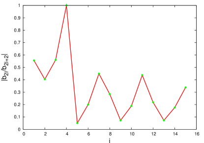
Figure 2: Ratio $b_{2i}/b_{2i+2}$ of the Taylor expansion coefficients of the potential as a function of $i$.

From Tabular 1 we estimate that the radius of convergence of the Taylor series (24), given by

$$r=\lim_{i\to\infty}\frac{b_{2i}}{b_{2i+2}},$$ (27)

is finite. This can be seen more clearly from Fig. 2, where we plotted the ratios $b_{2i}/b_{2i+2}$ as functions of $i$. Note, that for the corresponding series with dimensionful field and couplings $\bar{b}_{2i}=b_{2i}\cdot k^{3/2-i}$ the radius of convergence shrinks with decreasing scale $k$,

$$\bar{r}=\lim_{i\to\infty}\frac{\bar{b}_{2i}}{\bar{b}_{2i+2}}=k\lim_{i\to\infty}\frac{b_{2i}}{b_{2i+2}}=k\cdot r\,.$$ (28)

Thus, the radius of convergence of the power series expansion of $W^{\prime}_{k}(\phi)$ tends to zero for $k\to 0$.

III.1.2 Partial differential equation

Let us now turn to the solution of the partial differential equation (22). We have seen in Eq. (III.1.1) that the coupling associated with the IR unstable direction does not feed back into the fixed-point equation. It is therefore sufficient to consider the second derivative of Eq. (22). To simplify the notation we introduce $u(\varphi)=w^{\prime\prime}_{k}(\varphi)$. The fixed-point equation for $u$ reads

$$u^{\prime\prime}=2u\,\frac{u^{2}-3}{u^{4}-1}\,u^{\prime\,2}+4\pi^{2}\frac{(u^{2}+1)^{2}}{u^{2}-1}(2u-\varphi u^{\prime}).$$ (29)

It is straightforward to see that the above equation has an asymptotic solution $u_{\rm as}(\varphi)\sim\varphi^{2}$. Employing a standard Runge-Kutta solver for ordinary differential equations we find one regular odd solution for the starting condition $u(0)=0$ and $u^{\prime}(0)\equiv 2\lambda\approx\pm 2\cdot 1.59508=\pm 3.19016\,.$ For field amplitudes $\varphi<0.245$ the regular solution is bounded by $u<1$ and this inner part of the solution corresponds to the IR stable fixed-point solution found in the polynomial approximation discussed above.

Since $u=w^{\prime\prime}$ we find for large fields

$$w^{\prime\prime}(\varphi\to\pm\infty)\simeq\pm\,\varphi^{2}\Longrightarrow W^{\prime\prime}_{\ast}(\phi\to\pm\infty)\simeq\pm\,\phi^{2}.$$

In other words the outer part of the regular fixed-point solution connects smoothly to the inner part. Thus we have found a solution corresponding to a bosonic potential $V\simeq(k^{3/2}w^{\prime}_{\ast}(\varphi))^{2}$ which behaves as $\sim\phi^{6}$ for large $\phi$. This is the supersymmetric analogue of the Wilson-Fisher fixed point of three-dimensional $O(N)$ theories, see e. g. Tetradis:1993ts ; Berges:2000ew .

III.2 Next-to-leading order

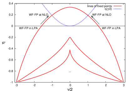
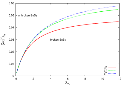
Figure 3: Left panel: Lines of fixed points in the $\eta$-$\gamma$ plane (solid curves) and the anomalous dimension as a function of $\gamma=2\lambda$ as obtained from Eq. (34) (dotted curve). Right panel: Phase diagram in the plane spanned by the dimensionless couplings specified at the cutoff scale $\Lambda$ as obtained from truncations with $n=1$ ($\phi^{2}$), $n=2$ ($\phi^{4}$), and $n=3$ ($\phi^{6}$) in Eq. (24).

For the next-to-leading order approximation we employ the following ansatz

$$\begin{split}\Gamma_{k}=\int d^{3}x\left(\frac{1}{2}Z_{k}^{2}\left(\partial_{\mu}\phi\partial^{\mu}\phi-i\bar{\psi}\not{\partial}\psi F^{2}\right)\right.\\ \left.+FW_{k}^{\prime}(\phi)-\frac{1}{2}W_{k}^{\prime\prime}(\phi)\bar{\psi}\psi\right)\,,\end{split}$$ (30)

with $Z_{k}^{2}$ being a scale-dependent wave-function renormalization. We neglect a possible momentum and $\phi$ dependence of $Z_{k}$. This approximation corresponds to an inclusion of the next-to-leading order correction in a systematic expansion of the effective action in powers of fields and derivatives. As we discuss below, we find that the anomalous dimension $\eta$ remains small compared to one within this approximation, see also Tabular 3. Thus, we expect that higher-order corrections such as $\sim(\phi\partial_{\mu}\phi)^{2}$ does not significantly affect our results for the zero- and finite-temperature phase diagram.

Projecting on the part linear in the auxiliary field and integrating with respect to $\phi$ yields the superpotential. On the other hand projecting on the terms quadratic in the auxiliary fields yields the flow equation for the wave function renormalization. Employing the regulator functions (19) we find the following coupled set of differential equations:

$$\partial_{k}W_{k}(\phi)= -\frac{k^{2}W^{\prime\prime}_{k}(\phi)}{24\pi^{2}}\,\frac{k\partial_{k}Z_{k}^{2}+3Z_{k}^{2}}{k^{2}Z_{k}^{4}+W^{\prime\prime}_{k}(\phi)^{2}}\,,$$ (31)

$$\partial_{k}Z_{k}^{2}= -\frac{k^{2}}{4\pi^{2}}(k\partial_{k}Z_{k}^{2}+2Z_{k}^{2})\times$$

$$\left.\times\frac{Z_{k}^{2}W_{k}^{(3)}(\phi)^{2}\left(k^{2}Z_{k}^{4}-W_{k}^{\prime\prime}(\phi)^{2}\right)}{\left(k^{2}Z_{k}^{4}+W_{k}^{\prime\prime}(\phi)^{2}\right)^{3}}\right|_{\phi=0}\,.$$ (32)

Introducing the anomalous dimension $\eta=-\partial_{t}\ln Z_{k}^{2}$ and the dimensionless quantities

$$\chi=Z_{k}k^{-\frac{1}{2}}\phi,\quad\mathfrak{w}(\chi)=k^{-2}W_{k}(\phi),\quad$$

the dimensionless flow equations read

$$\partial_{t}\mathfrak{w}+2\mathfrak{w} =\frac{1}{2}(1+\eta)\chi\,\mathfrak{w}-\frac{(3-\eta)\mathfrak{w}^{\prime\prime}}{24\pi^{2}(1+\mathfrak{w}^{\prime\prime 2})}\,,$$ (33)

$$\eta =\left.\frac{(2\!-\!\eta)(1\!-\!\mathfrak{w}^{\prime\prime 2})\mathfrak{w}^{\prime\prime\prime 2}}{4\pi^{2}(1\!+\!\mathfrak{w}^{\prime\prime 2})^{3}}\right|_{\chi=0}\!\!\!\!\!\!\!\!\!\!.$$ (34)

In order to study the fixed-point structure it is convenient to consider the anomalous dimension $\eta$ as a free parameter, see e. g. Ref. Neves:1998tg . In complete analogy to the two-dimensional Wess-Zumino model we find lines of fixed points corresponding to potentials with no nodes (outermost line), one node and so on, see Fig. 3 (left panel). In fact, we encounter exactly the same picture as in two dimensions, apart from a shift of the graph to lower $\eta$ values. Concerning the number of fixed points the situation is completely different as in two dimensions: Because of the shift of $\eta$ we find only one pair of fixed points for $\eta=0$, and not an infinite number of pairs. Such a dependence on the dimensionality has also been observed for $O(N)$ models Neves:1998tg .

Note that if we had actually used the same regulator as in Synatschke:2009nm , namely

$$r_{1}=0\quad\hbox{and}\quad r_{2}=\left(\frac{k^{2}}{p^{2}}-1\right)\theta(k^{2}-p^{2}),$$

then the flow equation for the superpotential in two dimensions would turn into the flow equation in three dimensions under the transformation $\eta\to\eta-1$. This correspondence explains the similarities of Fig. 3 (left panel) in two and three dimensions.

As in two dimensions, we can deduce a superscaling relation from the RG flow equation of $a^{2}$ which relates the critical exponent $1/{\nu_{\rm{}_{W}}}$ and the anomalous dimension Gies:2009az :

$$\frac{1}{\nu_{\rm{}_{W}}}=\frac{3-\eta}{2}\,.$$ (35)

The truncation dependence of the fixed-point value of the anomalous dimension is shown in Tabular 3.

$2n$	4	6	8	10	12	14
$\eta_{*}$	0.187711	0.188258	0.18802	0.187996	0.188001	0.188003

Table 3: Dependence of the fixed-point value of the anomalous dimension $\eta$ on the truncation order $n$ of the expansion of $w^{\prime}$ in powers of the field $\varphi$, see also Eq. (24).

III.3 Zero-temperature phase diagram and scaling of the mass

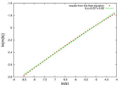
Figure 4: Logarithm of the boson mass as a function of the RG-scale $k$. A linear fit to the data points yields $m(k)\sim k^{0.23}$ for $k\ll\Lambda$.

The breaking of supersymmetry is driven by the unstable direction $a^{2}$, similarly as in two dimensions Synatschke:2009nm . In the plane spanned by the values of the dimensionless couplings $\lambda$ and $\lambda a^{2}$ given at the cutoff-scale $\Lambda$ we find a transition line for supersymmetry breaking, see Fig. 3 (right panel).

From the effective potential $V=\lim_{k\to 0}W^{\prime 2}_{k}/2$, we read off the mass of the boson,

$$m^{2}_{\rm bos}=W^{\prime}_{k\to 0}(\phi_{0})\,W^{\prime\prime\prime}_{k\to 0}(\phi_{0})+W^{\prime\prime\,2}_{k\to 0}(\phi_{0})\,,$$ (36)

where the field $\phi_{0}$ minimizes $V$. In the case of broken supersymmetry (and unbroken $\mathbbm{Z}_{2})$ we have $\phi_{0}=0$ and the mass is given by

$$m^{2}_{{\rm broken}}=W^{\prime}_{k\to 0}(0)W^{\prime\prime\prime}_{k\to 0}(0),\quad W^{\prime\prime}_{k\to 0}(0)=0,$$ (37)

whereas for unbroken supersymmetry it is given by

$$m_{\rm unbroken}^{2}=W^{\prime\prime\,2}_{k\to 0}(\phi_{0}),\quad W^{\prime}_{k\to 0}(\phi_{0})=0\,.$$ (38)

In the broken phase a polynomial expansion of the superpotential is justified and we find

$$m_{{\rm broken}}^{2}(k)=W_{k}^{\prime}(0)W_{k}^{\prime\prime\prime}(0)=2k^{2}\lambda^{2}a^{2}\,.$$ (39)

From the scaling of the couplings for $k\to 0$,

$$\lambda_{\ast}\sim\text{const.}\quad\text{and}\quad a^{2}\sim k^{-\frac{3}{2}}\,,$$ (40)

we read off that the mass scales as

$$m(k)\sim k^{\frac{1}{4}}\quad\hbox{for}\quad k\ll\Lambda\,.$$ (41)

This scaling behavior is demonstrated in Fig. 4 for a truncation with $n=4$, i. e. an expansion of $w^{\prime}$ up to order $\varphi^{8}\sim\phi^{8}$, see also Eq. (24). Due to our analysis of the convergence of the fixed-point values of the couplings $\lambda$ and $b_{2i}$ as well as the anomalous dimension $\eta_{*}$, see Tabular 1, 2 and 3, we expect that the truncation order $n=4$ is already sufficient to capture qualitatively and quantitatively most of the features of the zero- and finite-temperature phase diagram, see also Sect. IV.2. From a linear fit to the double-logarithmic plot of $m(k)$ we find $m(k)\sim k^{0.23}$ which is indeed reasonably close to the expected scaling given in Eq. (41). The reason for this behavior, which is very different from the one found in $O(N)$ models, is that the unstable direction does not feed back into the fixed-point equation. Independent of the value of the coupling at the UV (ultraviolet) cutoff scale $\Lambda$, the second derivative of the superpotential flows always into its IR fixed point corresponding to a conformally invariant theory. In $O(N)$ models, on the other hand, the unstable direction in the broken regime feeds back into the fixed-point equations for the couplings. Approaching the IR fixed point of $O(N)$ models requires therefore fine tuning of the UV parameters Tetradis:1993ts .

IV Flow equations at finite temperature

In this section we study finite temperature effects in the three-dimensional Wess-Zumino model. To this end we restrict ourselves to the LPA which we expect to provide already a quantitative insight into the finite-temperature phase structure as shown in Ref. Braun:2009si .

The finite-temperature flow equation in LPA can be obtained straightforwardly from the zero-temperature equations (20) by replacing the momentum integration in time-like direction by a summation over Matsubara frequencies:

$$p_{0}\longrightarrow\left\{\begin{array}[]{c}\nu_{n}\\ \omega_{n}\end{array}\right\}\,,\quad\int\frac{dp_{0}}{2\pi}\dots\longrightarrow T\sum_{n=-\infty}^{\infty}\dots$$ (42)

with frequencies $\omega_{n}=2\pi nT$ for bosonic fields and $\nu_{n}=(2n+1)\pi T$ for fermionic fields. We refer to Appendix B for a detailed derivation of the finite-temperature flow equations. Here we simply note that we can perform the Matsubara sums explicitly for the regulator functions (18). The flow equations read

$$\partial_{k}{W^{\prime}_{k}}^{\rm bos}= -\frac{k^{2}}{8\pi^{2}}W_{k}^{\prime\prime\prime}\frac{k^{2}-W^{\prime\prime 2}_{k}}{(k^{2}+W^{\prime\prime 2}_{k})^{2}}\times$$ (43)

$$\left(\frac{\pi T}{k}-(2s_{\rm B}+1)^{2}\frac{\pi T}{k}+2(2s_{\rm B}+1)\right)\frac{\pi T}{k}\,,$$

$$\partial_{k}{W^{\prime}_{k}}^{\rm ferm}= -\frac{k^{2}}{8\pi^{2}}\frac{(k^{2}-W^{\prime\prime 2}_{k})W_{k}^{\prime\prime\prime}}{(k^{2}+W^{\prime\prime 2}_{k})^{2}}\biggl{(}\!1-\Bigl{(}1-\frac{2s_{\rm F}\pi T}{k}\Bigr{)}^{2}\biggr{)},$$ (44)

where the temperature-dependent floor functions $s_{\rm B}$ and $s_{\rm F}$ are given by

$$s_{\rm B}=\left\lfloor\frac{k}{2\pi T}\right\rfloor\quad\text{and}\quad s_{\rm F}=\left\lfloor\frac{k}{2\pi T}+\frac{1}{2}\right\rfloor\,.$$ (45)

The differences in the flow equations for the ’superpotential’ describing the self-interaction of bosons and the ’superpotential’ describing the Yukawa-type interaction between fermions and bosons originates in the supersymmetry breaking induced by the different thermal boundary conditions for the bosonic and fermionic fields.

IV.1 Pressure

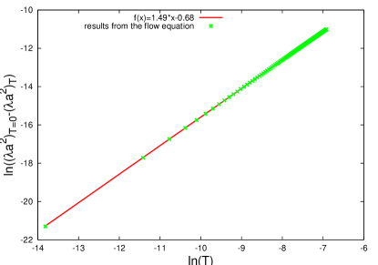
Figure 5: Double logarithmic plot of the temperature dependent minimum of the superpotential versus the temperature.

In the previous section we have shown that the boson mass tends to zero for $k\to 0$ in the phase with broken supersymmetry (restored $\mathbbm{Z}_{2}$ symmetry). Thus we expect that the thermodynamic properties of the three-dimensional model in the phase with restored $\mathbbm{Z}_{2}$ symmetry are similar to that of a gas of massless bosons. The pressure of such a gas in $2+1$ dimensions is given by

$$\Delta p=\frac{\zeta(3)}{2\pi}\,T^{3}.$$ (46)

The (normalized) pressure $\Delta p$ for a given temperature is determined by the negated difference of the interaction potential for a given temperature evaluated at the minimum and its corresponding zero-temperature value. In our model this corresponds to the height of the barrier in the double-well potential $(W^{\prime})^{2}$ for a theory with broken $\mathbb{Z}_{2}$ symmetry or the minimum of $(W^{\prime})^{2}$ with unbroken $\mathbb{Z}_{2}$ symmetry. For small temperatures we therefore expect

$$\Delta(\lambda a^{2})\equiv (\lambda a^{2})_{T=0}-(\lambda a^{2})_{T\neq 0}$$

$$= \sqrt{\frac{\zeta(3)}{2\pi}}\cdot T^{\frac{3}{2}}\simeq\exp(-0.83)T^{\frac{3}{2}}\,$$ (47)

for the temperature dependence of the minimum of $W^{\prime}(\phi)$. In Fig. 5 we show the double-logarithmic plot of the minimum of the superpotential versus temperature as obtained from a truncation of the potential with $n=4$, i. e. an expansion of $w^{\prime}$ up to order $\varphi^{8}\sim\phi^{8}$, see also Eq. (24). The linear fit to the double-logarithmic plot yields a power law $\Delta(\lambda a^{2})=\exp(-0.68)\cdot T^{1.49}$ which is compatible with the values for a gas of massless bosons in $2+1$ dimensions, as given in Eq. (47). We expect that deviations from the ideal gas limit are present for two reasons: (i) The boson mass tends to zero for $k\to 0$ only but remains finite for any $k>0$, see Eq. (41) and (ii) boson self-interactions lead to deviations from the ideal bose-gas limit.

IV.2 RG flows at finite temperature and dimensional reduction

For high temperatures $T\gg k$ both floor functions in (45) vanish and the flow equations simplify considerably:

$$\partial_{k}{W^{\prime}_{k}}^{\rm bos} =-\frac{k^{2}}{8\pi^{2}}W_{k}^{\prime\prime\prime}\frac{k^{2}-W^{\prime\prime 2}_{k}}{(k^{2}+W^{\prime\prime 2}_{k})^{2}}\frac{2\pi T}{k}\,,$$ (48)

$$\partial_{k}{W^{\prime}_{k}}^{\rm ferm} =0\,.$$ (49)

Following Ref. Tetradis:1992xd we rescale the quantities in the bosonic flow equation according to

$$\phi = \sqrt{T}\tilde{\phi},\quad W_{k}(\phi)=T\tilde{W}_{k}(\tilde{\phi})\,.$$ (50)

For Eq. (48) this leads exactly to the zero-temperature flow equation of the two-dimensional model. At this point, however, we should stress that the theory which we obtain in the limit $T/k\gg 1$ is not the supersymmetric $\mathcal{N}=1$ Wess-Zumino model in two dimensions since the fermions have dropped out of the theory due to the absence of thermal zero-modes. Therefore supersymmetry is necessarily broken at finite temperature. The fact that we still obtain the same functional form for the bosonic flow equation can be understood in terms of the role of the auxiliary field: In order to obtain the bosonic flow equation, we have to project on the terms coupling to the auxiliary field. Since there is no coupling between the auxiliary field and the fermionic part of the theory, the fermions do not contribute to the bosonic flow equation.

Because of the rescalings of the fields and the potential according to Eq. (50) we expect that the couplings exhibit the following behavior for $T/k\gg 1$:

$${{}^{3D}}(a^{2})_{T} ={{}^{2D}(a^{2})_{T=0}}\left(\frac{T}{k}\right)^{1/2},$$

$${{}^{3D}}\lambda_{T} ={{}^{2D}}\lambda_{T=0}\left(\frac{T}{k}\right)^{-1/2},$$ (51)

$${{}^{3D}}(b_{2i})_{T} ={{}^{2D}}(b_{2i})_{T=0}\left(\frac{T}{k}\right)^{1/2-i},$$

where ${{}^{2D}(a^{2})_{T=0}},\,{{}^{2D}}\lambda_{T=0}$ and ${{}^{2D}}(b_{2i})_{T=0}$ denote the fixed-point values of the couplings of the two-dimensional theory. Indeed we observe such a running of the couplings for $T/k\gg 1$ in our numerical studies.

From Eq. (IV.2) we deduce the radius of convergence of our expansion of the potential in powers of the fields. Recalling the relation between the dimensionful and dimensionless couplings, $\bar{b}_{2i}=b_{2i}\cdot k^{\,3/2-i}$, we find

$${}^{3D}r= \lim_{i\to\infty}\frac{{}^{3D}{(\bar{b}_{2i})_{T}}}{{}^{3D}{(\bar{b}_{2i+2})_{T}}}$$

$$= \lim_{i\to\infty}\frac{{}^{2D}{(b_{2i})_{T=0}}\cdot(T/k)^{1/2-i}\cdot k^{\,3/2-i}}{{}^{2D}{(b_{2i+2})_{T=0}}\cdot(T/k)^{-1/2-i}\cdot k^{\,1/2-i}}$$ (52)

$$= {{}^{2D}}r\cdot T\,.$$

Thus we find a finite radius of convergence for the polynomial expansion of the superpotential at finite temperature which is a consequence of the finite radius of convergence found for the underlying two-dimensional model at zero temperature Synatschke:2009nm . However, the radius of convergence ${}^{3D}r$ tends to zero for $T\to 0$, in full agreement with our results in Sect. III.1.

IV.3 Phase diagram at finite temperature

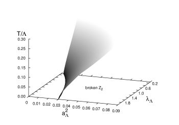
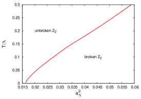
Figure 6: Finite-temperature phase diagram of the ${\mathcal{N}}=1$ Wess-Zumino model. Left panel: $\mathbbm{Z}_{2}$ phase boundary in the space spanned by temperature $T/\Lambda$ and the value of the couplings $(\lambda_{\Lambda},a^{2}_{\Lambda})$ at vanishing temperature. Right panel: Slice of the $\mathbbm{Z}_{2}$ phase-boundary for fixed $\lambda_{\Lambda}=0.8$.

In this subsection we discuss the phase diagram of the ${\mathcal{N}}=1$ Wess-Zumino model at finite temperature.

Whether supersymmetry is broken or not at vanishing temperature depends on our choice for the couplings at the cutoff scale as we have discussed above. At finite temperature we have necessarily soft supersymmetry breaking due to the different boundary conditions for bosons and fermions in Euclidean time direction. Besides supersymmetry, however, our theory is invariant under $\phi\to-\phi$. At vanishing temperature the breakdown of this ${\mathbb{Z}}_{2}$ symmetry is intimately linked to the question whether supersymmetry is broken or not. Recall that at $T=0$ broken $\mathbbm{Z}_{2}$-symmetry of the ground state implies a supersymmetric ground state and that restored $\mathbbm{Z}_{2}$ symmetry of the ground state implies broken supersymmetry. Even though supersymmetry is necessarily broken at finite temperature, we shall see in the following that $\mathbbm{Z}_{2}$ symmetry of the ground state can be either broken or restored depending on the actual value of the temperature. Due to the relation between supersymmetry and ${\mathbb{Z}}_{2}$ symmetry at vanishing temperature, we consider the strength of ${\mathbb{Z}}_{2}$ breaking as a measure for supersymmetry breaking at finite temperature. Thus we distinguish between the case of soft supersymmetry breaking due to finite temperature but broken $\mathbbm{Z}_{2}$ symmetry of the ground state and the case with restored $\mathbbm{Z}_{2}$ symmetry of the ground state at finite temperature.

For our numerical study of the finite-temperature phase diagram we employ a $\phi^{8}$-truncation of the potentials, i. e. we use $n=4$ in Eq. (24).

In the left panel of Fig. 6, we show the ${\mathbb{Z}}_{2}$ phase-boundary in the space spanned by temperature $T/\Lambda$ and the value of the couplings $(\lambda_{\Lambda},a^{2}_{\Lambda})$ at the UV cutoff scale at vanishing temperature. The lower end of the phase boundary on the $T=0$ plane in Fig. 6 corresponds to the phase-transition line which separates the phase with broken supersymmetry from the one associated with a supersymmetric ground state, see also Fig. 3 (right panel). Choosing couplings $(\lambda_{\Lambda},a^{2}_{\Lambda})$ at $T=0$ associated with a supersymmetric ground state (and broken $\mathbbm{Z}_{2}$ symmetry) we find always a second-order phase-transition temperature at which the system enters the phase with restored $\mathbbm{Z}_{2}$ symmetry. As discussed in Sect. IV.1 the thermodynamic properties of this $\mathbbm{Z}_{2}$-symmetric phase are similar to the ones of a gas of massless bosons. We expect that this finite-temperature phase transition falls into the Ising universality class with critical exponents determined by the underlying 2$d$ $\mathbbm{Z}_{2}$ theory, namely by the exponents of Onsager’s solution of the corresponding lattice spin model. However, a quantitative analysis of the critical behavior would require the inclusion of the anomalous dimension in our studies. This is deferred to future work.

In the right panel of Fig. 6, we show a slice of the $\mathbbm{Z}_{2}$ phase boundary for fixed $\lambda_{\Lambda}=0.8$. We find that the phase-transition temperature increases with increasing $(a^{2}_{\Lambda})_{T=0}$. Since $(a^{2}_{k\to 0})_{T=0}$ increases with increasing $(a^{2}_{\Lambda})_{T=0}$, the phase-transition temperature increases with increasing $(a^{2}_{k\to 0})_{T=0}$, i. e. in terms of the renormalized quantity. Our observation of an increasing phase-transition temperature with increasing $(a^{2}_{k\to 0})_{T=0}$ is in accordance with our expectations from a scalar $O(1)\simeq\mathbbm{Z}_{2}$ model since $(\lambda_{*}a^{2}_{k\to 0})_{T=0}$ sets the scale at $T=0$ and therefore plays a similar role as a finite expectation value of the fields in $O(N)$ models, see e. g. Bohr:2000gp .

V Conclusions

In this work we have employed the functional RG for a study of the three dimensional $\mathcal{N}=1$ Wess-Zumino model at zero and at finite temperature. Since the model exists only in Minkowski space we have worked with a formulation of the Wetterich equation in Minkowski-space and have Wick-rotated the momentum integrals.

At zero temperature we have found results quite similar to our findings for the two-dimensional model Synatschke:2009nm . An investigation of the fixed point structure yields the supersymmetric analogue of the Wilson-Fisher fixed-point for bosonic theories. It is maximally IR stable with one relevant direction only. As in the two-dimensional model the relevant direction is given by $a^{2}$. Again we find a scaling relation between the critical exponent $1/\nu_{\rm{}_{W}}$ of the instable direction and the anomalous dimension $\eta$. The critical exponent $\nu_{\rm{}_{W}}$ governs the freeze-out of the minimum of the superpotential $W$. We also find that the IR limit of the three-dimensional Wess-Zumino model is given by a conformally invariant theory. The critical exponent $\nu_{\rm{}_{W}}$ governs the vanishing of the mass with the RG scale. This is different from three-dimensional scalar $O(N)$ theories since for the supersymmetric models the relevant coupling does not feed back in the flow equations of higher $n$-point functions. As in two dimensions we find that supersymmetry breaking is governed by the relevant direction.

The finite-temperature flow equations are obtained by replacing the integration over the time-like direction by a sum over Matsubara frequencies. As bosons and fermions obey different thermal boundary conditions, finite temperatures introduce a soft supersymmetry breaking.

In the phase with broken supersymmetry (restored $\mathbbm{Z}_{2}$ symmetry) at zero temperature the three-dimensional Wess-Zumino model flows to a massless field theory. In the $\mathbbm{Z}_{2}$ symmetric phase at finite temperature the model therefore behaves like a three-dimensional gas of massless bosons. We have found that this is indeed the case. The small deviations from the ideal-gas law found in our numerical studies originate from the self-interaction of the bosons.

At high temperatures, supersymmetry breaking manifests itself in the fact that the flow equations for the superpotential, derived from the bosonic and the fermionic part of the action, are different. We also observe dimensional reduction in the way that, after a suitable rescaling, the flow equation for the ”bosonic” superpotential in three dimensions reduces to the flow equation in two dimensions. Due to the absence of a fermionic thermal zero-mode the fermions do not contribute to the RG flow for small scales $k\ll T$. We have argued that the radius of convergence for the polynomial expansion of the superfield interpolates between the values for two and three dimensions as the temperature is raised.

Even though supersymmetry is explicitly broken at finite temperature, the $\mathbbm{Z}_{2}$ symmetry of the model can be either restored or broken at finite temperature. Whether $\mathbbm{Z}_{2}$ symmetry is broken or not depends on the temperature (and parameters of the model, i. e. the initial values of the couplings at the initial RG scale). Since supersymmetry and $\mathbbm{Z}_{2}$ symmetry are intimately linked we have argued that a study of $\mathbbm{Z}_{2}$ symmetry may be used to measure the strength of supersymmetry breaking. We have computed the phase diagram for the restoration of $\mathbb{Z}_{2}$ symmetry at finite temperatures. We find two different types of phases which are separated by a second order phase transition: one phase with soft supersymmetry breaking due to finite temperature but broken $\mathbbm{Z}_{2}$ symmetry and one with restored $\mathbbm{Z}_{2}$ symmetry.

Throughout this paper we have addressed several similarities and differences between scalar $O(N)$ models and the ${\mathcal{N}}=1$ Wess-Zumino model at zero and finite temperatures, e. g. the fixed-point structure at zero temperature and the behavior at finite temperature. A detailed exploration of both models with respect to their similarities and differences, in particular with respect to the large-$N$ limit, is deferred to future work.

Appendix A Derivation of the flow equations in Minkowski space

In this Addendum we derive the Wetterich flow equation in Minkowski space. For the sake of simplicity we consider a real scalar field in this appendix. The generalization to other fields, such as fermion or gauge fields, is straightforward.

The generating functional in Minkowski-space is given by

$$Z[J]=\int\mathcal{D}\varphi\,e^{i(S[\varphi]+(J,\varphi))}\,,$$

where $J$ denotes the external source and $(J,\varphi)\equiv\int d^{d}x\,J(x)\varphi(x)$. The generating functional $W$ for the connected two-point functions, the so-called Schwinger functional, reads

$$W[J]=i\ln Z[j]\,.$$

From this we obtain

$$\frac{\delta}{\delta J}W[J] =i\frac{\delta}{\delta J}\ln Z[J]=-\frac{\int\mathcal{D}\phi\,e^{i(S+\int J\phi)}\phi}{\int\mathcal{D}\phi\,e^{i(S+(J,\varphi))}}$$

$$=-\phi=-\langle{\varphi}\rangle\,.$$

The effective action is the Legendre transform of the Schwinger functional,

$$\Gamma[\phi]=-W[J]-(J,\phi)\,,$$

where $\phi$ is the mean (classical) field. Using $\frac{\delta}{\delta J}W[J]=-\phi$, we obtain the equation of motion for the field $\phi$:

$$\frac{\delta\Gamma[\phi]}{\delta\phi} =-\int d^{d}y\frac{\delta W[J]}{\delta J(y)}\frac{\delta J(y)}{\delta\phi(x)}-\int d^{d}y\frac{\delta J(y)}{\delta\phi(x)}\phi(y)-J(x)$$

$$=-J(x)\,.$$

The scale-dependent generating functional is defined as

$$Z_{k}[J]= e^{-iW_{k}[J]}=e^{i\Delta S_{k}[\frac{\delta}{\delta J}]}Z[J]$$

$$= \int\mathcal{D}\varphi\,e^{i(S[\varphi]+\int_{x}\varphi J+\Delta S_{k}[\varphi])}$$

with

$$\Delta S_{k}[\phi]=\frac{1}{2}\int\frac{d^{4}q}{(2\pi)^{4}}\varphi(-q)R_{k}(q)\varphi(q)\,.$$

Here, the momentum-dependent regulator function $R_{k}$ provides an IR cutoff for all modes and has to satisfy three conditions: (i) $R_{k}(p)|_{p^{2}/k^{2}\to 0}>0$ which implements the IR regularization, (ii) $R_{k}(p)|_{k^{2}/p^{2}\to 0}=0$ which ensures that the regulator vanishes for $k\to 0$, (iii) $R_{k}(p)|_{k\to\Lambda\to\infty}\to\infty$ which ensures that the path integral is dominated by the stationary point for $k\to\Lambda\to\infty$. Different choices for $R_{k}$ define different RG trajectories manifesting the RG scheme dependence, but the IR physics $\Gamma_{k\to 0}\to\Gamma$ should remain invariant provided the truncation captures all relevant operators for the physical observables under investigation. In turn, a variation of the regulator function may lead to more insight on the truncation dependence of our results.

Next, we define the scale-dependent effective action:

$$\Gamma_{k}[\phi]=-W_{k}[J]-\int d^{4}x\,J\phi-\Delta S_{k}[\phi]\,.$$

In order to properly formulate the flow equations in Minkowski-space we have to take $k^{2}\sim p_{\mu}p^{\mu}$ as flow parameter. Therefore we define $\partial_{t}=2k^{2}\partial_{k^{2}}$ to be the derivative with respect to RG ’time’ $t=\ln k^{2}$. Taking the derivative of $\Gamma_{k}[\phi]$ with respect to $t$ yields

$$\partial_{t}\Gamma_{k}[\phi]=-\partial_{t}W_{k}[J]-\partial_{t}\int d^{4}xJ\phi-\partial_{t}\Delta S_{k}[\phi]\,,$$ (53)

where we have used that the source is independent of $k$. For the derivative of $W_{k}$ we obtain

$$\partial_{t}W_{k}[J]=i\partial_{t}\ln Z[J]$$

$$=\frac{i}{Z[J]}\int\mathcal{D}\varphi\frac{i}{2}\int\frac{d^{d}q}{(2\pi)^{d}}\varphi\partial_{t}R_{k}\varphi e^{i(S[\varphi]+\int_{x}\varphi J+\Delta S_{k}[\varphi])}$$

$$=-\frac{1}{2Z[J]}\int\frac{d^{d}q}{(2\pi)^{d}}\partial_{t}R_{k}{\int\mathcal{D}\varphi\;\varphi\,\varphi\,e^{i(S[\varphi]+\int_{x}\varphi J+\Delta S_{k}[\varphi])}}$$

$$=\frac{1}{2Z[J]}\int\frac{d^{d}q}{(2\pi)^{d}}(\partial_{t}R_{k})\frac{\delta^{2}Z[J]}{\delta J\delta J}\,.$$

Using the definition of the Schwinger functional, $Z_{k}[J]=e^{-iW_{k}}$, we find

$$\partial_{t}W_{k}[J]=e^{iW_{k}}\frac{1}{2}\int\frac{d^{d}q}{(2\pi)^{d}}(\partial_{t}R_{k})\frac{\delta^{2}e^{-iW_{k}}}{\delta J\delta J}\,.$$ (54)

Now we rewrite the integrand by making use of

$$\frac{\delta^{2}e^{-iW_{k}}}{\delta J\delta J} =\frac{\delta}{\delta J}e^{-iW_{k}}(-i)\frac{\delta W_{k}}{\delta J}$$

$$=e^{-iW_{k}}(-i)\frac{\delta W_{k}}{\delta J}(-i)\frac{\delta W_{k}}{\delta J}+e^{-iW_{k}}(-i)\frac{\delta^{2}W_{k}}{\delta J\delta J}\,,$$

then Eq. (54) can be rewritten as follows:

$$\partial_{t}W_{k}[J]= \frac{1}{2}\int\frac{d^{d}q}{(2\pi)^{d}}\partial_{t}R_{k}\biggl{(}-\underbrace{\frac{\delta W_{k}}{\delta J}}_{-\phi}\underbrace{\frac{\delta W_{k}}{\delta J}}_{-\phi}-i\frac{\delta^{2}W_{k}}{\delta J\delta J}\biggr{)}$$

$$= -\Delta S_{k}-\frac{i}{2}\int\frac{d^{d}q}{(2\pi)^{d}}\partial_{t}R_{k}\frac{\delta^{2}W_{k}}{\delta J\delta J}\,.$$

With this relation the variation of the effective action Eq. (53) takes the form

$$\partial_{t}\Gamma_{k}[\phi]=\frac{i}{2}\int\frac{d^{d}q}{(2\pi)^{d}}(\partial_{t}R_{k})\frac{\delta^{2}W_{k}}{\delta J\delta J}\,.$$

The second functional derivative of $W$ with respect to the source $J$ can be written in terms of the effective action:

$$\frac{\delta^{2}\Gamma_{k}}{\delta\phi\delta\phi} =-\frac{\delta J}{\delta\phi}-R_{k}$$

$$\Rightarrow\frac{\delta J}{\delta\phi} =-\left(\frac{\delta^{2}W_{k}}{\delta J\delta J}\right)^{-1}=-\left(\frac{\delta^{2}\Gamma_{k}}{\delta\phi\delta\phi}+R_{k}\right)\,.$$ (55)

Making use of

$$\delta(q-q^{\prime})=\frac{\delta\phi(q)}{\delta\phi(q^{\prime})}= -\frac{\delta}{\delta\phi}\frac{\delta W_{k}}{\delta J}=-\int\frac{d^{d}q}{(2\pi)^{d}}\frac{\delta^{2}W_{k}}{\delta J\delta J}\frac{\delta J}{\delta\phi}\,,$$

we obtain the Wetterich equation in Minkowski-Space:

$$\partial_{t}\Gamma_{k}[\phi]=\frac{i}{2}\,{\rm Tr}\,\biggl{[}(\partial_{t}R_{k})\Bigl{(}\frac{\delta^{2}\Gamma_{k}}{\delta\phi\delta\phi}+R_{k}\Bigr{)}^{-1}\biggr{]}\,.$$ (56)

Appendix B Derivation of the flow equations at finite temperature

In order to preserve supersymmetry in the RG flow for vanishing temperature, we must choose a regulator function which regularizes the theory in the time-like direction and the space-like directions in the same way. In order to make apparent how soft SUSY-breaking due to finite temperature emerges, we use the same regulator for our finite-temperature and zero-temperature studies. It is given by:

$$r_{2}=\left(\frac{k}{|p|}-1\right)\theta\left(\frac{p^{2}}{k^{2}}-1\right),\quad r_{1}=0\,.$$

In the LPA, the finite-temperature flow equations can be obtained straightforwardly from the zero-temperature flow equations by replacing $p_{0}$ by the Matsubara modes $\nu_{n}$ and $\omega_{n}$ of fermion and boson fields, respectively, and replacing the integration over $p_{0}$ by a summation over the Matsubara modes. The contribution of the bosons to the RG flow of our Wess-Zumino model then reads:

$$\partial_{k}W_{k}^{\prime}=W_{k}^{\prime\prime\prime}T\sum_{n=-\infty}^{\infty}\int\frac{d^{2}p_{s}}{8\pi^{2}}\frac{(W^{\prime\prime 2}_{k}-k^{2})\theta(k^{2}-p_{s}^{2}-\omega_{n}^{2})}{(k^{2}+W^{\prime\prime 2}_{k})^{2}\sqrt{p_{s}^{2}+\omega_{n}^{2}}}\,,$$

where $p_{s}$ denotes the momenta in space-like directions. Along the lines of, e. g., Gies:1999vb , we use Poisson’s sum formula,

$$\sum_{n=-\infty}^{\infty}f(n)=\sum_{\ell=-\infty}^{\infty}\int_{-\infty}^{\infty}dqf(q)\exp(-2\pi i\ell q)\,,$$

in order to obtain

$$\partial_{k}W_{k}^{\prime}= W_{k}^{\prime\prime\prime}T\sum_{\ell=-\infty}^{\infty}\int_{-\infty}^{\infty}dq\int\frac{d^{2}p_{s}}{8\pi^{2}}\times$$

$$\frac{(W^{\prime\prime 2}_{k}-k^{2})\theta(k^{2}-p_{s}^{2}-(2\pi qT)^{2})}{(k^{2}+W^{\prime\prime 2}_{k})^{2}\sqrt{p_{s}^{2}+(2\pi qT)^{2}}}{\rm e}^{-2\pi iq\ell}\,.$$

For the computation of the three-dimensional integral, we first substitute $q^{\prime}=2\pi Tq$ and introduce spherical coordinates

$$p_{s}^{1}=r\cos\vartheta\sin\varphi,\;p_{s}^{2}=r\sin\vartheta\sin\varphi,\;q^{\prime}=r\cos\vartheta.$$

Performing the angular integrations yields

$$\partial_{k}W_{k}^{\prime}=W_{k}^{\prime\prime\prime}T\sum_{\ell=-\infty}^{\infty}\int_{0}^{k}\frac{dr}{8\pi^{2}T}\frac{(W^{\prime\prime 2}_{k}-k^{2})}{(k^{2}+W^{\prime\prime 2}_{k})^{2}}\frac{2T\sin(\frac{\ell r}{T})}{\ell}\,.$$

Finally the integration over $r$ leads to

$$\partial_{k}W_{k}^{\prime}=\frac{(W^{\prime\prime 2}_{k}-k^{2})W_{k}^{\prime\prime\prime}}{8\pi^{2}(k^{2}+W^{\prime\prime 2}_{k})^{2}}\,2T^{2}\sum_{\ell=-\infty}^{\infty}\frac{1-\cos(\frac{\ell k}{T})}{\ell^{2}}\,.$$

Since we made use of Poisson’s resummation formula to rewrite the sum over the thermal modes, we are able to split the flow equation into a zero-temperature and a finite-temperature contribution:

$$\partial_{k}W_{k}^{\prime}=\frac{(W^{\prime\prime 2}_{k}-k^{2})W_{k}^{\prime\prime\prime}}{8\pi^{2}(k^{2}+W^{\prime\prime 2}_{k})^{2}}\biggl{(}k^{2}+\underbrace{4T^{2}\sum_{\ell=1}^{\infty}\frac{1-\cos(\frac{k\ell}{T})}{\ell^{2}}}_{g_{\rm bos}(T)}\biggr{)}\,.$$

The contribution of the fermions to the RG flow of our model can be obtained along the lines of our derivation of the bosonic contribution and reads:

$$\partial_{k}W_{k}^{\prime}=\frac{(W^{\prime\prime 2}_{k}-k^{2})W_{k}^{\prime\prime\prime}}{8\pi^{2}(k^{2}+W^{\prime\prime 2}_{k})^{2}}\biggl{(}\!k^{2}+\underbrace{4T^{2}\sum_{\ell=1}^{\infty}(-)^{\ell}\frac{1-\cos(\frac{k\ell}{T})}{\ell^{2}}}_{g_{\rm ferm}(T)}\biggr{)}\,.$$

Introducing the dimensionless temperature $\tilde{T}=T/k$, the functions $g_{\rm bos}(T)$ and $g_{\rm ferm}(T)$ can be written in terms of Polylogarithms:

$$g_{\rm bos}(\tilde{T})= \frac{2}{3}k^{2}\tilde{T}^{2}\left[\pi^{2}-3\mathrm{Li}_{2}({\rm e}^{-{\rm i}/\tilde{T}})-3\mathrm{Li}_{2}({\rm e}^{{\rm i}/\tilde{T}})\right]\,,$$

$$g_{\rm ferm}(\tilde{T})= -\frac{2}{6}k^{2}\tilde{T}^{2}\left[\pi^{2}+6\mathrm{Li}_{2}(-{\rm e}^{-{\rm i}/\tilde{T}})+6\mathrm{Li}_{2}(-{\rm e}^{{\rm i}/\tilde{T}})\right]\,.$$

Using the identity Lewin:1981

$$\mathrm{Li}_{2}\left(-z\right)+\mathrm{Li}_{2}\left(-\frac{1}{z}\right) =2\mathrm{Li}_{2}(-1)-\frac{1}{2}\ln^{2}(z)$$

$$=-\frac{\pi^{2}}{6}-\frac{1}{2}\ln^{2}(z)\,,$$

the function $g_{\rm bos}(T)$ simplifies further to

$$g_{\rm bos}(\tilde{T}) =\tilde{T}^{2}\left[\pi^{2}+\ln^{2}\big{(}-\exp(i/\tilde{T})\big{)}\right]$$

$$=\pi T\left(\pi T-(2s_{B}+1)^{2}\pi T+(2s_{B}+1)2k\right)-k^{2}\,,$$ (57)

where we have used that

$$\ln\left(\exp(i/\tilde{T}+i\pi)\right)=\frac{i}{\tilde{T}}-i\pi\,(2s_{B}+1),$$

$$s_{B}\leq\frac{1}{2\pi\tilde{T}}\leq s_{B}+1\;\Rightarrow\;s_{B}=\left\lfloor\frac{k}{2\pi T}\right\rfloor\,.$$

Similarly, exploiting the relation

$$\ln\left(\exp(i/\tilde{T})\right)=\frac{i}{\tilde{T}}-2i\pi\,s_{F},$$

$$s_{F}-\frac{1}{2}\leq\frac{1}{2\pi\tilde{T}}\leq s_{F}+\frac{1}{2}\;\Rightarrow\;s_{F}=\left\lfloor\frac{k}{2\pi T}+\frac{1}{2}\right\rfloor\,,$$

we end up with the result

$$g_{\rm ferm}(T)=-k^{2}\left(1-s_{F}\frac{2\pi T}{k}\right)^{2}$$

for the fermions. As expected, the functions $g_{\rm bos}(T)$ and $g_{\rm ferm}(T)$ exhibit the same behavior as the threshold functions discussed in Ref. Litim:2001up .

References

- (1) K. Aoki. Introduction to the nonperturbative renormalization group and its recent applications. Int. J. Mod. Phys., B14:1249–1326, 2000.
- (2) Jurgen Berges, Nikolaos Tetradis, and Christof Wetterich. Non-perturbative renormalization flow in quantum field theory and statistical physics. Phys. Rept., 363:223–386, 2002. hep-ph/0005122.
- (3) Daniel F. Litim and Jan M. Pawlowski. On gauge invariant Wilsonian flows. 1998. hep-th/9901063
- (4) Jan M. Pawlowski. Aspects of the functional renormalisation group. Annals Phys., 322:2831–2915, 2007.
- (5) Holger Gies. Introduction to the functional RG and applications to gauge theories. 2006. hep-ph/0611146
- (6) Hidenori Sonoda. The Exact Renormalization Group – renormalization theory revisited –. 2007. arXiv:0710.1662 [hep-th]
- (7) Janos Polonyi. Lectures on the functional renormalization group method. Central Eur. J. Phys., 1:1–71, 2003.
- (8) Bertrand Delamotte. An introduction to the nonperturbative renormalization group. 2007. cond-mat/0702365
- (9) F. Vian. Supersymmetric gauge theories in the exact renormalization group approach. 1998. hep-th/9811055
- (10) M. Bonini and F. Vian. Wilson renormalization group for supersymmetric gauge theories and gauge anomalies. Nucl. Phys., B532:473–497, 1998.
- (11) Oliver J. Rosten. On the Renormalization of Theories of a Scalar Chiral Superfield. 2008. arXiv:0808.2150 [hep-th]
- (12) Hidenori Sonoda and Kayhan Ulker. Construction of a Wilson action for the Wess-Zumino model. Prog. Theor. Phys., 120:197–230, 2008.
- (13) Franziska Synatschke, Holger Gies, and Andreas Wipf. Phase Diagram and Fixed-Point Structure of two dimensional N=1 Wess-Zumino Models. Phys. Rev., D80:085007, 2009.
- (14) Holger Gies, Franziska Synatschke, and Andreas Wipf. Supersymmetry breaking as a quantum phase transition. Phys. Rev., D80:101701, 2009.
- (15) Franziska Synatschke, Georg Bergner, Holger Gies, and Andreas Wipf. Flow Equation for Supersymmetric Quantum Mechanics. JHEP, 03:028, 2009.
- (16) N. Tetradis and C. Wetterich. Critical exponents from effective average action. Nucl. Phys., B422:541–592, 1994.
- (17) Daniel F. Litim. Critical exponents from optimised renormalisation group flows. Nucl. Phys., B631:128–158, 2002.
- (18) Claude Bervillier, Andreas Juttner, and Daniel F. Litim. High-accuracy scaling exponents in the local potential approximation. Nucl. Phys., B783:213–226, 2007.
- (19) Jean Pierre Derendinger and Claudio Lucchesi. Realizations of thermal supersymmetry. Nucl. Phys., B536:483–510, 1998.
- (20) Ashok K. Das and Michio Kaku. Supersymmetry at High Temperatures. Phys. Rev., D18:4540, 1978.
- (21) L. Girardello, Marcus T. Grisaru, and P. Salomonson. Temperature and Supersymmetry. Nucl. Phys., B178:331, 1981.
- (22) Shoichi Midorikawa. Behavior of Supersymmetry at Finite Temperature. Prog. Theor. Phys., 73:1245, 1985.
- (23) Detlev Buchholz and Izumi Ojima. Spontaneous collapse of supersymmetry. Nucl. Phys., B498:228–242, 1997.
- (24) Daniel F. Litim. Optimisation of the exact renormalisation group. Phys. Lett., B486:92–99, 2000.
- (25) Daniel F. Litim. Optimised renormalisation group flows. Phys. Rev., D64:105007, 2001.
- (26) Jens Braun and Holger Gies. Chiral phase boundary of QCD at finite temperature. JHEP, 06:024, 2006.
- (27) Daniel F. Litim and Jan M. Pawlowski. Non-perturbative thermal flows and resummations. JHEP, 11:026, 2006.
- (28) D. F. Litim and J. M. Pawlowski, Predictive power of renormalisation group flows: A comparison. Phys. Lett., B516:197–207, 2001.
- (29) Jean-Paul Blaizot, Andreas Ipp, Ramon Mendez-Galain, and Nicolas Wschebor. Perturbation theory and non-perturbative renormalization flow in scalar field theory at finite temperature. Nucl. Phys., A784:376–406, 2007.
- (30) Stefan Floerchinger, Michael Scherer, Sebastian Diehl, and Christof Wetterich. Particle-hole fluctuations in the BCS-BEC Crossover Phys. Rev., B78:174528, 2008
- (31) Sebastian Diehl, Stefan Floerchinger, Holger Gies, Jan M. Pawlowski, and Christof Wetterich. Functional renormalization group approach to the BCS-BEC crossover 2009. arXiv:0907.2193 [cond-mat.quant-gas]
- (32) Jens Braun. Thermodynamics of QCD low-energy models and the derivative expansion of the effective action. 2009. arXiv:0908.1543 [hep-th]
- (33) N. Tetradis and C. Wetterich. The high temperature phase transition for phi**4 theories. Nucl. Phys., B398:659–696, 1993.
- (34) O. Bohr, B. J. Schaefer, and J. Wambach. Renormalization group flow equations and the phase transition in O(N) models. Int. J. Mod. Phys., A16:3823–3852, 2001.
- (35) F. Benitez, J. P. Blaizot, H. Chate, B. Delamotte, R. Mendez-Galain and N. Wschebor, Solutions of renormalization group flow equations with full momentum dependence. Phys. Rev. E, 80:030103, 2009 [arXiv:0901.0128 [cond-mat.stat-mech]].
- (36) A. C. Lehum. Dynamical generation of mass in the D = (2+1) Wess-Zumino model. Phys. Rev., D77:067701, 2008.
- (37) Christof Wetterich. Exact evolution equation for the effective potential. Phys. Lett., B301:90–94, 1993.
- (38) Jurgen Berges and Gabriele Hoffmeister. Nonthermal fixed points and the functional renormalization group. Nucl. Phys., B813:383–407, 2009.
- (39) Rui Neves, Yuri Kubyshin, and Robertus Potting. Polchinski ERG equation and 2D scalar field theory. 1998. hep-th/9811151
- (40) G. Papp, B. J. Schaefer, H. J. Pirner, and J. Wambach. On the convergence of the expansion of renormalization group flow equation. Phys. Rev., D61:096002, 2000.
- (41) Holger Gies. QED effective action at finite temperature: Two-loop dominance. Phys. Rev., D61:085021, 2000.
- (42) Leonard Lewin. Polylogarithms and Associated Functions. North Holland, pages 1–380, 1981.