Self-consistent Simulations of Alfvén Wave Driven Winds

Abstract

We review our recent results of Alfvén wave-driven winds. First, we present the result of a self-consistent 1D MHD simulations for solar winds from the photosphere to interplanetary region. Here, we emphasize the importance of the reflection of Alfvén waves in the density stratified corona and solar winds. We also introduce the recent HINODE observation that might detect the reflection signature of transverse (Alfvénic ) waves by Fujimura & Tsuneta (2009). Then, we show the results of Alfvén wave-driven winds from red giant stars. We explain the change of the atmosphere properties from steady coronal winds to intermittent chromospheric winds and discuss how the wave reflection is affected by the decrease of the surface gravity with stellar evolution. We also discuss similarities and differences of accretion disk winds by MHD turbulence.

1 Introduction

The main difficulty of the coronal heating and solar wind acceleration is how to lift up nonthermal (e.g. magnetic) energy from the photosphere to upper regions because the hotter corona cannot stably exist above the cooler photosphere by upward thermal heat flux. In addition, it is not well understood how to let the energy dissipate at appropriate positions. The origin of energy that heats up the corona and accelerates the solar winds is in the surface convective layer. The solar atmosphere is filled with complicated structure of magnetic field which is supposed to be amplified by dynamo mechanism in the interior (e.g., Brun et al., 2004). The turbulent motions of the surface convection drive various modes of upward propagating waves. The turbulent motions may also trigger magnetic reconnections which result in flares and flare-like events, which drive various mode of waves at locations above the photosphere (Sturrock, 1999). In this paper, we focus on the roles of the waves in heating and accelerating the solar winds.

The compressive waves that are excited at the photosphere cannot travel to sufficiently upper regions because they easily steepen the wave fronts to form shocks after the amplification of the amplitude in the density decreasing atmosphere. For instance, the acoustic waves mostly dissipate before reaching the corona, and therefore they cannot contribute to the heating of the corona and the acceleration of the solar wind (Stein & Schwartz, 1972; Suzuki, 2002). Fast mode waves in low $\beta$ (magnetically dominated) condition suffer refraction so that they hardly reach the coronal height if the fast mode speed varies in horizontal direction due to complicated magnetic structure (Khomenko & Collados, 2006). In general, the compressive waves that are excited from the photosphere cannot give a significant contribution to the coronal heating and solar wind acceleration.

On the other hand, Alfvén waves can travel a longer distance owing to the incompressive characters. A fraction of the Alfvén waves excited at the photospheric level is supposed to propagate to the corona and the solar wind acceleration region so that they play a more dominant role in the heating and acceleration of the solar wind than the compressive waves. Alfvénic oscillations are also detected in various regions on the Sun by the recent observations using the HINODE satellite, e.g., in a solar prominence (Okamoto et al., 2007), in spicules (De Pontieu et al., 2007), and in a chromospheric jet (Nishizuka et al., 2008).

To understand the dissipation mechanism of the Alfvén waves is a key to understand the heating and acceleration of the solar wind because this corresponds to the transfer of the energy flux of the Alfvén waves to the ambient plasma. The Alfvén speed in general largely changes with height because the density and magnetic field strength decrease in a different manner. Shiota et al. (2010) have estimated the distribution of Alfvén speeds in a polar region from HINODE observation and found that the Alfvén speeds actually vary in both vertical and horizontal directions. Under these circumstances, Alfvén waves suffer reflection through the upward propagation as a result of the deformation of the wave shape (An et al., 1990; Moore et al., 1991; Hollweg & Isenberg, 2007). Interactions between the outgoing Alfvén waves and the incoming component possibly lead to the damping through turbulent-like cascade (e.g., Dmitruk et al., 2003; Cranmer, et al., 2007; Verdini & Velli, 2007). This process might further generate high-frequency ioncyclotron waves, which are widely discussed especially on the preferential heating of the perpendicular components with respect to magnetic field of minor heavy ions (e.g., Tu & Marsch, 1997; Kohl et al., 1998; Cranmer, et al., 1999). The variation of the Alfvén speeds also anticipate phase mixing of Alfvén waves along neighboring field lines (Heyvaerts & Priest, 1983; Sakurai & Granik, 1984; Voitenko & Goossens, 2005), which might further generate fast mode waves (Nakariakov et al., 1997). The density stratification and the variation of the Alfvén speed also enhances the parametric decay instability of outgoing Alfvén waves (Suzuki & Inutsuka 2006; SI06 hereafter). The parametric decay excites compressive waves in addition to incoming Alfvén waves. In contrast to those excited at the photosphere, these compressive waves are generated in the upper regions and directly contribute to the heating of the corona and solar winds by the shock dissipation.

Although the final wave dissipation mechanism and heating process are still not well figured out, understanding the wave reflection in stratified atmosphere with varying Alfvén speed is primarily important. Alfvén waves are reflected most effectively in the chromosphere and transition region because of the rapid change of the density. While most of the Alfvén waves from the surface cannot penetrate into the corona, the remaining waves sufficiently heat and accelerate the solar wind. Our previous work (Suzuki & Inutsuka 2005; SI05 hereafter) showed that the transmitted fraction into the corona is an order of 10$\%$ and that this is enough for the coronal heating and solar wind acceleration in open coronal holes. Although turbulent-like cascade of Alfvén (ic) waves is not treated in this work because we adopted one dimensional (1D) magnetohydrodynamical (MHD) simulations, this is the first attempt that dynamically treats wave reflection from the photosphere to solar wind regions simultaneously with heating of the gas by the wave damping. In this review paper, we firstly summarize our dynamical simulations of solar winds, focusing on the reflection of Alfvén waves under various conditions. Actually, the recent HINODE observation also detected a signature of reflected Alfvén waves (Fujimura & Tsuneta, 2009), which will be introduced in more detail later.

The concept of Alfvén wave-driven winds is not limited to the Sun. It is expected that the similar mechanism operates in winds from other stars (e.g. Velli, 1993), such as protostars (Cranmer, 2008), low- and intermediate-mass main sequence stars, red giant stars (Suzuki, 2007, S07 hereafter), and proto-neutron stars with strong magnetic field (Suzuki & Nagataki 2005). Among these objects, we show Alfvén wave driven red giant winds in this paper based on our work (S07). In red giant stars, the stratification properties (e.g. decrease of density) of the atmosphere are different from those in the Sun because of the smaller surface gravity. This affects the propagation and reflection of the Alfvén waves. Here we discuss the change of the wave reflection with stellar evolution.

In the last part of this paper, we further extend to winds from accretion disks. To date, it has been widely discussed that accretion disk winds can be driven by centrifugal force (Blandford & Payne, 1982; Kudoh & Shibata, 1998). Global magnetic field plays a key role in this process; if there is poloidal field that is sufficiently tilted with respect to an accretion disk, the gas can flow out along with the field lines. On the other hand, it is expected that small-scale MHD turbulence also potentially drives disk winds, similarly to the solar winds, although such mechanism has not been well studied so far. It is now widely accepted that the outward transport of disk angular momentum and inward mass accretion are realized by the effective viscosity owing to turbulence. Magnetorotational instability (MRI) is now known to be a very effective mechanism that drives turbulence if weak magnetic fields exist initially (Balbus & Hawley 1991). The excited MHD turbulence is supposed to accelerate the disk material to upper regions as well as transport the angular momentum outwardly. In Suzuki & Inutsuka (2009), we studied the disk winds driven by MHD turbulence by local disk simulations. In this paper, we introduce the results with emphasizing the similarity to and difference from the Alfvén wave-driven solar and stellar winds.

2 Solar Winds

2.1 Simulation Set-up

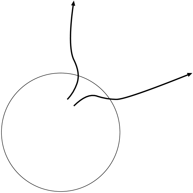
Figure 1: Set-up of solar wind simulations. The cartoon shows a schematic view of a super-radially open flux tube, which we set in our simulations.

We simulate the heating and acceleration of solar winds in 1D super-radially expansing flux tubes from the photosphere to sufficiently distant locations (0.1 – 0.3 AU). Here we summarize the basic points of the simulation set-up. For the details, please see SI05 and SI06. We determine radial magnetic field strength, $B_{r}$, from the conservation of magnetic flux :

$$B_{r}fr^{2}={\rm const.},$$ (1)

where $r$ is heliocentric distance, and $f$ is a super-radial expansion factor. We give radial variation of $f$ in advance. The structure of $B_{r}(r)$ is determined by surface radial field, $B_{r,0}$, and $f$, and is fixed during the simulations. In our simulations (SI05 & SI06), we consider the magnetic field of $\sim$ few hundred Gauss for $B_{r,0}$ and the total super-radial expansion factor of 75-450, which give the average magnetic field strength of open field regions, $B_{r,0}/f$, of an order of 1 G. We should remark that recent HINODE observations found that open magnetic flux tubes in polar regions are connected to ubiquitously distributed unipolar patches with more than kilo-Gauss (Tsuneta el al., 2008; Shiota et al., 2010). These open flux tubes super-radially open with a factor of several hundred to a thousand. Although the obtained $B_{r,0}$ and $f$ are slightly larger than those adopted in our simulations, the values of the average strength, $B_{r,0}/f$, are similar. As shown in SI06 and Suzuki (2006), $B_{r,0}/f$ is a more important parameter in determining the properties of the solar winds.

We inject transverse perturbations of magnetic field with various spectra from the photosphere. Outgoing Alfvén waves are excited by these fluctuations. The propagation and dissipation of the waves are dynamically treated by the following MHD equations :

$$\frac{d\rho}{dt}+\frac{\rho}{r^{2}f}\frac{\partial}{\partial r}(r^{2}fv_{r})=0,$$ (2)

$$\rho\frac{dv_{r}}{dt}=-\frac{\partial p}{\partial r}-\frac{1}{8\pi r^{2}f}\frac{\partial}{\partial r}(r^{2}fB_{\perp}^{2})+\frac{\rho v_{\perp}^{2}}{2r^{2}f}\frac{\partial}{\partial r}(r^{2}f)-\rho\frac{GM_{\odot}}{r^{2}},$$ (3)

$$\rho\frac{d}{dt}(r\sqrt{f}v_{\perp})=\frac{B_{r}}{4\pi}\frac{\partial}{\partial r}(r\sqrt{f}B_{\perp}).$$ (4)

$$\rho\frac{d}{dt}\left(e+\frac{v^{2}}{2}+\frac{B^{2}}{8\pi\rho}-\frac{GM_{\odot}}{r}\right)+\frac{1}{r^{2}f}\frac{\partial}{\partial r}\left[r^{2}f\left\{\left(p+\frac{B^{2}}{8\pi}\right)v_{r}\right.\right.$$

$$\left.\left.-\frac{B_{r}}{4\pi}(\mbox{\boldmath${B\cdot v}$})\right\}\right]+\frac{1}{r^{2}f}\frac{\partial}{\partial r}(r^{2}fF_{\rm c})+q_{\rm R}=0,$$ (5)

$$\frac{\partial B_{\perp}}{\partial t}=\frac{1}{r\sqrt{f}}\frac{\partial}{\partial r}[r\sqrt{f}(v_{\perp}B_{r}-v_{r}B_{\perp})],$$ (6)

where $\rho$, ${v}$, $p$, ${B}$ are density, velocity, pressure, and magnetic field strength, respectively, and subscripts $r$ and $\perp$ denote radial and tangential components; $\frac{d}{dt}$ and $\frac{\partial}{\partial t}$ denote Lagrangian and Eulerian derivatives, respectively; $e=\frac{1}{\gamma-1}\frac{p}{\rho}$ is specific energy and we assume the equation of state for ideal gas with a ratio of specific heat, $\gamma=5/3$; $G$ and $M_{\odot}$ are the gravitational constant and the solar mass; $F_{\rm c}(=\kappa_{0}T^{5/2}\frac{dT}{dr})$ is thermal conductive flux by Coulomb collisions, where $\kappa_{0}=10^{-6}$ in c.g.s unit (Braginskii, 1965); $q_{\rm R}$ is radiative cooling. We use optically thin radiative loss (Landini & Monsignori-Fossi, 1990) in the corona and take into account optically thick effects in the chromosphere (Anderson & Athay, 1989; Moriyasu et al., 2004, SI06).

We adopt the second-order MHD-Godunov-MOCCT scheme to update the physical quantities. Each cell boundary is treated as discontinuity, and for the time evolution we solve nonlinear Riemann shock tube problems with the magnetic pressure term by using the Rankin-Hugoniot relations. Therefore, heating is automatically calculated from the shock jump condition. A great advantage of our code is that no artificial viscosity is required even for strong MHD shocks; numerical diffusion is suppressed to the minimum level for adopted numerical resolution.

We initially set static atmosphere with a temperature $T=10^{4}$K to see whether the atmosphere is heated up to coronal temperature and accelerated to a transonic flow. At $t=0$ we start the inject of the transverse fluctuations from the photosphere and continue the simulations until the quasi-steady states are achieved.

2.2 Results

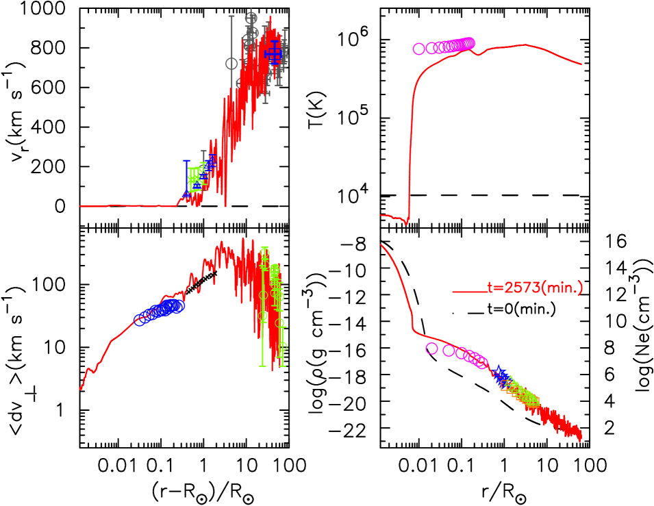
Figure 2: Comparison of the simulation result with observations of fast solar wind. Outflow speed, $v_{r}$(km s^-1) (Top-left), temperature, $T$(K) (top-right), rms transverse amplitude, $\langle dv_{\perp}\rangle$(km s^-1) (bottom-left), and density in logarithmic scale, $\log(\rho({\rm g\;cm^{-3}}))$ (bottom-right), are plotted. Observational data in the temperature panel are electron density, $\log(N_{e}({\rm cm^{-3}}))$ which is to be referred to the right axis. Dashed lines indicate the initial conditions and solid lines are the results at $t=2573$ minutes. In the bottom panel, the initial value ($\langle dv_{\perp}\rangle=0$) dose not appear. Top-left: Green vertical error bars are proton outflow speeds in an interplume region by UVCS/SoHO (Teriaca et al., 2003). Dark blue vertical error bars are proton outflow speeds by the Doppler dimming technique using UVCS/SoHO data (Zangrilli et al., 2002). A dark blue open square with errors is velocity by IPS measurements averaged in 0.13 - 0.3AU of high-latitude regions (Kojima et al., 2004). Light blue data are taken from Grall et al. (1996); crossed bars are IPS measurements by EISCAT, crossed bars with open circles are by VLBA measurements, and vertical error bars with open circles are data based on observation by SPARTAN 201-01 (Habbal et al., 1994). top-right: Pink circles are electron temperatures by CDS/SoHO (Fludra et al., 1999). bottom-left: Blue circles are non-thermal broadening inferred from SUMER/SoHO measurements (Banerjee et al., 1998). Cross hatched region is an empirical constraint of non-thermal broadening based on UVCS/SoHO observation (Esser et al., 1999). Green error bars are transverse velocity fluctuations derived from IPS measurements by EISCAT(Canals et al., 2002). bottom-right: Circles and stars are observations by SUMER/SoHO (Wilhelm et al., 1998) and by CDS/SoHO (Teriaca et al., 2003), respectively. Triangles (Teriaca et al., 2003) and squares (Lamy et al., 1997) are observations by LASCO/SoHO.

Before discussing the reflection of the Alfvén waves in various cases, we explain how the coronal heating and the solar wind acceleration were accomplished in the typical case which we studied in SI05 and SI06 for the fast solar wind. We adopt $B_{r,0}=161$ G, the total $f=75$, and the root-mean-squared (rms) surface amplitude, $\langle dv\rangle=0.7$ km s^-1. Figure 2 plots the final structure of the simulated solar wind after the quasi-steady state is achieved in comparison with observations of fast solar winds. In the four panels $v_{r}$(km s^-1), $T$(K), mass density, $\rho$(g cm^-3), and rms transverse amplitude, $\langle dv_{\perp}\rangle$(km s^-1) are plotted. As for the density, we compare our result with observed electron density, $N_{e}$, in the corona. When deriving $N_{e}$ from $\rho$ in the corona, we assume H and He are fully ionized, and $N_{e}({\rm cm^{-3}})=6\times 10^{23}\rho$(g cm^-3).

Figure 2 shows that the initially cool and static atmosphere is effectively heated and accelerated by the dissipation of the Alfvén waves. The sharp TR which divides the cool chromosphere with $T\sim 10^{4}$K and the hot corona with $T\sim 10^{6}$K is formed owing to a thermally unstable region around $T\sim 10^{5}$K in the radiative cooling function (Landini & Monsignori-Fossi, 1990). The hot corona streams out as the transonic solar wind. The simulation naturally explains the observed trend quite well. (see SI05 and SI06 for more detailed discussions.)

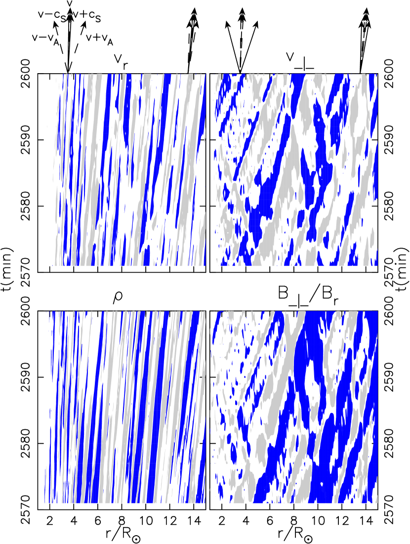
Figure 3: $r-t$ diagrams for $v_{r}$ (upper-left), $\rho$ (lower-left), $v_{\perp}$ (upper-right), and $B_{\perp}/B_{r}$ (lower-right.) The horizontal axises cover from $R_{\odot}$ to $15R_{\odot}$, and the vertical axises cover from $t=2570$ minutes to $2600$ minutes, where $R_{\odot}$ is the solar radius. Blue and gray shaded regions indicate positive and negative amplitudes which exceed certain thresholds. The thresholds are $dv_{r}=\pm 96$km/s for $v_{r}$, $d\rho/\rho=\pm 0.25$ for $\rho$, $v_{\perp}=\pm 180$km/s for $v_{\perp}$, and $B_{\perp}/B_{r}=\pm 0.16$ for $B_{\perp}/B_{r}$, where $d\rho$ and $dv_{r}$ are differences from the averaged $\rho$ and $v_{r}$. Arrows on the top panels indicate characteristics of Alfvén , slow MHD and entropy waves at the respective locations (see text).

The reflection of Alfvén waves are easily seen in $r-t$ diagrams. Figure 3 presents contours of amplitude of $v_{r}$, $\rho$, $v_{\perp}$, and $B_{\perp}/B_{r}$ in $R_{\odot}\leq r\leq 15R_{\odot}$ from $t=2570$ min. to $2600$ min. Blue (gray) shaded regions denote positive (negative) amplitude. Above the panels, we indicate the directions of the local 5 characteristics, two Alfvén , two slow, and one entropy waves at the respective positions. In our simple 1D geometry, $v_{r}$ and $\rho$ trace the slow modes which have longitudinal wave components, while $v_{\perp}$ and $B_{\perp}$ trace the Alfvén modes which are transverse (note that fast-mode and Alfvén mode degenerate in the simple 1D treatment, and then we simply call them Alfvén waves).

One can clearly see the Alfvén waves in $v_{\perp}$ and $B_{\perp}/B_{r}$ diagrams, which have the same slopes with the Alfvén characteristics shown above. One can also find the incoming modes propagating from lower-right to upper-left as well as the outgoing modes generated from the surface. These incoming waves are generated by the reflection at the ‘density mirrors’ of the slow modes in addition to the reflection owing to the shape deformation (SI05 & SI06). At intersection points of the outgoing and incoming characteristics the non-linear wave-wave interactions take place, which play a role in the wave dissipation.

The slow modes are seen in $v_{r}$ and $\rho$ diagrams. Although it might be difficult to distinguish, the most of the patterns are due to the outgoing slow modes which are generated from the perturbations of the Alfvén wave pressure, $B_{\perp}^{2}/8\pi$ (Kudoh & Shibata, 1999; Tsurutani et al., 2002). These slow waves steepen eventually and lead to the shock dissipation.

The processes discussed here are the combination of the direct mode conversion to the compressive waves and the parametric decay instability due to three-wave (outgoing Alfvén , incoming Alfvén , and outgoing slow waves) interactions (Goldstein, 1978; Terasawa et al., 1986) of the Alfvén waves. Although they are not generally efficient in the homogeneous background since they are the nonlinear mechanisms, the density gradient of the background plasma totally changes the situation. Owing to the gravity, the density rapidly decreases in the corona as $r$ increases, which results in the amplification of the wave amplitude so that the waves easily become nonlinear. Furthermore, the Alfvén speed varies a lot due to the change of the density even within one wavelength of Alfvén waves with periods of minutes or longer. This leads to both variation of the wave pressure in one wavelength and partial reflection through the deformation of the wave shape (Moore et al., 1991). The dissipation is greatly enhanced by the density stratification, in comparison with the case of the homogeneous background. Thus, the low-frequency Alfvén waves are effectively dissipated, which results in the heating and acceleration of the coronal plasma.

Figure 4: The top panels show the wave actions ($S_{\rm c}$) of the out-going (solid) and incoming (dashed) Alfvén waves. The bottom panels show density (solid) and temperature (dashed). The left panels are the results of the surface amplitude, $\langle dv\rangle=1.4$km s^-1, the middle panels are the results of $\langle dv\rangle=0.7$km s^-1, and the right panels are the results of $\langle dv\rangle=0.4$km s^-1.

From now, we examine how the reflection properties are affected by changing input parameters. In order to quantitatively study the dissipation and reflection of the Alfvén waves, we use an adiabatic constant, $S_{\rm c}$, of the outgoing Alfvén wave derived from wave action (Jacques, 1977):

$$S_{c,\pm}=\rho\langle\delta v_{\rm A,+}^{2}\rangle\frac{(v_{r}+v_{\rm A})^{2}}{v_{\rm A}}\frac{r^{2}f(r)}{r_{c}^{2}f(r_{c})},$$ (7)

where $v_{\rm A}=B_{r}/\sqrt{4\pi\rho}$ is Alfvén velocity and

$$\delta v_{\rm A,\pm}=\frac{1}{2}\left(v_{\perp}\mp B_{\perp}/\sqrt{4\pi\rho}\right)$$ (8)

is the amplitudes of the outgoing (for $+$ sign) and incoming (for $-$ sign) Alfvén waves (Elsässer variables).

First, we show the results with different values of surface fluctuations, $\langle dv\rangle=0.4,0.7,1.4$ km s^-1 (Figure 4). In the upper panel, we compare $S_{c,+}$ and $S_{c,-}$ of these three cases, whereas we use the absolute values for $S_{c,-}$ to show in logarithmic scale. As shown in the bottom panels, the density is very sensitive to the input $\langle dv\rangle$. The density of the $\langle dv\rangle=1.4$ km s^-1 case is 1000 times larger than the density of the $\langle dv\rangle=0.4$ km s^-1 case. Accordingly the mass fluxes of the solar winds differs about several hundred times. The differences of the densities and the mass fluxes between the two cases are much larger than the ratio of the input energy ($\propto dv^{2}$) $\approx 12$. The reasons why the density sensitively depends on the input surface perturbation can be explained by the reflection and the nonlinear damping of Alfvén waves.

The difference of the wave reflection in different $\langle dv\rangle$ cases are illustrated in the upper panels of Figure 4. In the smaller $\langle dv\rangle$ cases, the values of the outgoing (solid) and incoming (dashed) components are very similar especially in the chromospheric regions ($r-R_{\odot}\;\buildrel<\over{\sim}\;0.01R_{\odot}$). This indicates that most of the outgoing Alfvén waves generated from the surface is reflected back downward. Because the heating is smaller, the temperature is lower in the smaller $\langle dv\rangle$ cases. Then, the scale height becomes smaller and the density decreases rapidly. The Alfvén speed changes more rapidly and the wave shape is largely deformed, which enhances the reflection. When the input wave energy decreases, a positive feedback operates; a smaller fraction of the energy can reach the coronal region. As a result, the density and mass flux of the solar wind becomes much smaller than the decreasing factor of the input energy.

In addition to the effect of the wave reflection, the nonlinear dissipation of the Alfvén waves also plays a role in the sensitive behavior of the density on the input wave energy (SI06). When the input wave energy becomes smaller, the density becomes smaller as explained above. Then, the nonlinearity of Alfvén wave, $\delta v_{\rm A,+}/v_{\rm A}$, decreases not only because the amplitude, $\delta v_{\rm A,+}$, is small but also because the Alfvén speed, $v_{\rm A}(\propto 1/\sqrt{\rho})$, is larger. Therefore, the Alfvén waves do not dissipate and the heating is reduced, which further decreases the density; this is another type of positive feedbacks, which also results in the sensitive dependence of the density on the input wave energy.

Figure 5: Same as Figure 4 but for the cases with different spectra of surface perturbation. The left panels are the results of $P(\nu)\propto\nu^{-1}$ (pink noise), the middle panels are the results of $P(\nu)\propto\nu^{0}$ (white noise), and the right panels are the results of sinusoidal waves with 3 minutes.

Next, we investigate how the wave reflection is affected by the spectra of the input fluctuations. Here we study the three cases : The first case adopts the power spectrum, $P(\nu)\propto\nu^{-1}$ (pink noise), with respect to frequency, $\nu$; the second case adopts $P(\nu)\propto\nu^{0}$ (white noise); the third case adopts sinusoidal perturbation with period of 3 minutes. In the first and second cases, the range of the period is set from 20 seconds to 30 minutes. Figure 5 compares these three cases. The first and second cases show similar results, but in the chromospheric regions the first case suffers more reflection. This is because larger power is in longer wavelengths (lower frequency). If the wavelength is longer than the characteristic variation scale of Alfvén speed, Alfvén waves suffer more reflection.

The third case (sinusoidal perturbation) shows considerably different structure from these two cases. The transition region is not so sharp, which is seen in the temperature structure (dashed line in the bottom panel), because the heating is localized near the wave crests which are formed as a result of steepening of nonlinearly excited compressive waves. Then, the heating becomes more sporadic and responding to this intermittent heating the transition region moves up and down. This is a clear contrast to the first and second cases in which the sharp transition regions work as walls against the Alfvén waves because the Alfvén speeds change drastically. On the other hand, in the sinusoidal case Alfvén waves become more transmittant owing to the fluctuating transition region. As shown in the top panel, the reflected fraction (the ratio of the incoming component to the outgoing one in the chromosphere) is smaller in this case.

2.3 Discussions

2.3.1 Recent Observation of Waves

Wave activities are observed in various portions of the solar atmosphere. Propagating slow MHD waves are often observed in the corona as the fluctuations of intensity (Ofman et al., 1999; Sakurai et al., 2002; Banerjee et al., 2009). Tomczyk et al. (2007) detected Alfvén waves propagating along with magnetic field lines in the corona. Although the obtained wave amplitude is smaller than the value required for the coronal heating, this may be due to the line-of-sight effect (McIntosh et al., 2008). Indeed, nonthermal broadening of spectral lines, which are supposed to be closely linked to Alfvén waves, gives much larger amplitudes (Singh et al., 2004; Banerjee et al., 2009).

Alfvén (ic) waves are detected at the photospheric level in quiet regions (Ulrich, 1996) by analyzing the phase correlation of magnetic field and velocity perturbations. Similar attempts have been carried out in sunspot regions as well (Lites et al., 1998; Bellot Rubio et al., 2000), Recently, Fujimura & Tsuneta (2009) carried out very detailed analysis of the observed fluctuations by the spectro-polarimeter (SP) of the Solar Optical Telescope (SOT; Tsuneta et al., 2008; Suematsu et al., 2008; Ichimoto et al., 2008; Shimizu et al., 2008) aboard the HINODE satellite. They obtained the fluctuations of magnetic field, $\delta B$, the fluctuations of velocity field, $\delta v$, and the fluctuations of intensity, $\delta I$, which reflects density perturbation, $\delta\rho$ of pores, and magnetic concentrations in plages. The periods of the oscillations are distributed from 3 to 6 minutes in the pores and from 4 to 9 minutes in the plages. From the phase correlation of $\delta B$, $\delta v$, and $\delta I$ they investigated the modes and directions of the waves to that are attributed the observed fluctuations. One of the most important results is that the phase differences between $\delta v$ and $\delta B$ are nearly -90 degrees . The obtained phase correlation is consistent with standing kink-mode (transverse) or sausage-mode (longitudinal) waves, which are, roughly speaking, surface-mode counterparts of Alfvén and slow MHD waves. Namely, waves that propagate to positive and negative directions are almost equally exist at the photospheric level. Although it is quite difficult to estimate the fraction of sausage (compressive) mode and kink (nearly incompressive) mode because the transformation from $\delta I$ to $\delta\rho$ is not straightforward, it is expected that regions with smaller $\delta I$ are dominated by kink-mode oscillations. Based on this consideration, they picked up a particular pore region with relatively small $\delta I$. In this region, the phase difference between $\delta B$ and $\delta v$ is -96 degrees, which indicates that the upward propagating flux is slightly larger than the downward propagating component. Assuming the observed fluctuations attribute to kink-mode waves, they obtained the net Poynting flux that propagates upward as $2.7\times 10^{6}$ erg cm^-2s^-1.

Interestingly enough, our simulations also show very effective reflection of Alfvén waves below the transition region. In the reference case for the fast solar wind (Figure 2), 85% of the initial upward Poynting flux of the Alfvén waves from the photosphere is reflected back downward before reaching the corona. This implies that one can observe the comparable amount of downward flux to the upward component. The net leakage of the upgoing flux to the corona in this simulation is 15% of the input at the photosphere ($\sim 5\times 10^{5}$ erg cm^-2s^-1). These features seem quite consistent, at least in a qualitative sense, with the observation by Fujimura & Tsuneta (2009). The specific values of the leaking and reflected fluxes depend on strength and configuration of magnetic flux tubes and amplitudes of surface fluctuations.

2.3.2 Data Driven Simulations

The observation data are also used in numerical simulations. Recently, various groups are performing so-called data-driven simulations by adopting magnetic field data on the Sun (e.g. Manchester et al., 2008; Kataoka et al., 2009). While these works are mainly aiming at global heliospheric phenomena such as propagation of coronal mass ejections, observed data by HINODE are also applied for MHD simulations of surface activities. Matsumoto & Shibata (2009) have carried out numerical simulations in open field regions by using observed transverse motions on the Sun. They obtained horizontal motions of granules by local correlation tracking . These transverse motions are expected to excite Alfvénic waves that propagate along the vertical magnetic fields. They observed 14 different regions and derive the power spectrum of the transverse oscillations. Using the obtained spectrum as the input from the photosphere, they performed 1D MHD simulations in open field regions up to the corona following Kudoh & Shibata (1999). They found that, compared to artificial inputs of white noise or pink noise, more fraction of the Alfvén wave energy transmits through the transition region. They interpret that this is because more energy is resonantly trapped between the photosphere and the transition region and eventually leaks into the corona.

2.3.3 Slow Solar Winds

In this paper, we have introduced our simulation results for the fast solar winds from polar coronal holes. In SI06 and Suzuki (2006), we tried to explain observed data of slow solar winds in the same framework of the nonlinear dissipation of the Alfvén waves. We have shown that the slow winds from flux tubes with smaller $B_{r,0}/f$ and slightly larger $\langle dv_{\perp}\rangle$ well explain the observed properties of the slow streams from mid- to low-latitude regions; the same physical mechanism operates but the environments (e.g. geometries of flux tubes) make the differences between the fast and slow solar winds. This interpretation is quite consistent with the observed data by Interplanetary scintillation measurements (Kojima et al., 2005).

HINODE observations detected mass outflows from open regions in the vicinities of active regions (Sakao et al., 2007; Imada et al., 2007; Hara et al., 2008). These outflows might become slow solar winds and possibly give the significant contribution to the total mass loss from the Sun (Sakao et al., 2007). What is puzzling is that the acceleration seems to take place at a very low altitude. Harra et al. (2008) measured the Doppler velocities of the outflows and concluded that the outflow speeds reach $\approx 100$ km s^-1 at the height of $\sim 0.1R_{\odot}$ from the surface. Such rapid acceleration is very different from those inferred in the classical slow winds. For instance, the observations by Sheeley et al. (1997) shows that the slow winds associated with the streamer belt reach $\simeq 100$ km s^-1 above 2-3 solar radii.

It is difficult to explain the observed rapid acceleration by our simulations of the nonlinear Alfvén waves. If we increase the input energy ($\sim\langle dv^{2}\rangle$), density, rather than outflow speeds, increases owing to the larger heating. Probably other calculations or simulations will give similar tendency. To explain the outflow from the near active regions, pure momentum inputs are necessary.

3 Evolution to Red Giants

When the Sun evolve to a red giant star, the properties of the stellar wind also change. When the stellar atmosphere becomes cool enough to form dusts during the asymptotic giant branch (AGB), the stellar wind is mainly driven by the radiation pressure on the dust particles (Bowen, 1988). Before the AGB phase, namely from the main sequence to (early) red giant branch (RGB), the driving mechanism of the stellar winds is regarded to be similar to the solar wind; the origin of the driver is the kinetic energy of the surface convection, and MHD waves generated by the turbulent motion of the surface convection accelerates the stellar winds (e.g. Hartmann & MacGregor, 1980; Jatenco-Pereira & Opher, 1989; Charbonneau & MacGregor, 1995). However, the properties of the stellar winds change with stellar evolution primarily because the surface gravity decreases.

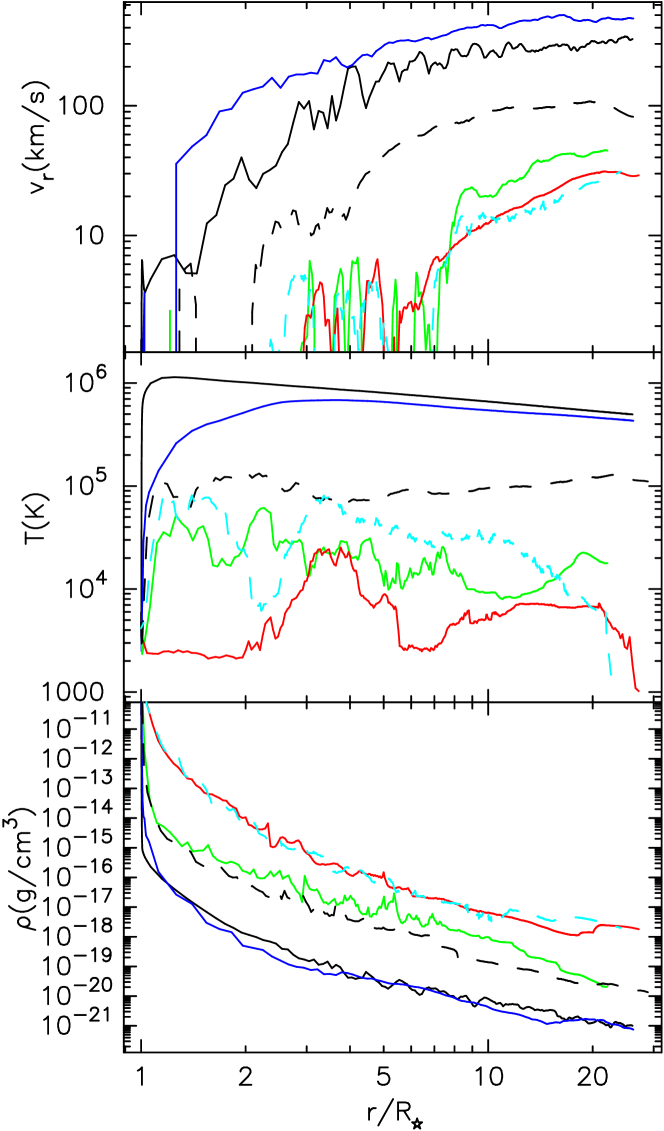
Figure 6: Evolution of stellar wind from the main sequence to RGB. From top to bottom, radial outflow velocity, $v_{r}$ (km s^-1), temperature, $T$ (K), and density, $\rho$(g cm^-3), are plotted. The solid lines are the results of the 1 $M_{\odot}$ stars ; the black, blue, green, and red lines are the results of the star with the surface gravity, $\log g=4.4$ (Sun), 3.4, 2.4, and 1.4, respectively. The dashed lines are the results of the $3\;M_{\odot}$ stars; the black and light-blue lines are the results of the stars with the surface gravity, $\log g=2.4$ and 1.4.

Based on these considerations, we studied the evolution of the stellar winds with the stellar evolution from the main sequence to the RGB (S07). We extend the solar wind simulation introduced in the previous section to simulate the red giant winds. We change the stellar radius, which controls the surface gravity, and effective temperature (or sound speed). We input the surface fluctuations that excite outgoing waves from the photosphere in the same manner as in the solar wind simulation. The amplitudes and spectra of the perturbations are estimated from the scaling relation of surface convective flux and period (Renzini et al., 1977, see also Brun & Palacios 2009 for recent simulations). We simulated the stellar winds from a $1M_{\odot}$ star with different surface gravities, $\log g=4.4$, 3.4, 2.4, and 1.4 (the Sun has $\log g=4.4$) to investigate the effect of the stellar evolution. In addition, we simulated the stellar winds from a $3M_{\odot}$ star with $\log=2.4$ and 1.4. In all the models we use the photospheric magnetic field, $B_{r,0}=240$ G, and the total super-radial expansion factor, $f=240$. Note that as for the main sequence star (the Sun in this case) these values are between the models for fast and slow solar winds (SI06). The stellar wind structures after the quasi-steady states are presented in Figure 6.

Figure 7: Cooling function of the solar metallicity gas from Landini & Monsignori-Fossi (1990). The main coolants in the respective temperature ranges are also indicated with arrows.

The figure shows that hot coronae with $T\;\buildrel>\over{\sim}\;10^{6}$ disappears when the star evolves to $\log g\leq 2.4$, and the density in the atmospheres and winds increase (when measured in stellar radii). The increase of the density is owing to the decrease of the surface gravity as a result of the expansion of the star; more mass can be lifted up to upper regions because of the smaller gravity. The decrease of the temperature can also be partly explained by the decrease of the gravity. When the star evolves to the red giant, the escape velocity becomes comparable to the sound speed; for example, the sound speed of the coronal gas ($\sim 150$ km s^-1) exceeds the escape speed of the red giant stars with $\log g\sim 2$ at a few stellar radii. Then, the hot corona with $T\;\buildrel>\over{\sim}\;10^{6}$ K cannot be confined by the gravity and inevitably streams out.

While the increase of the density is rather continuous with the stellar evolution, the temperature rapidly drops from the star with $\log g=3.4$ to the star with 2.4. Thermal instability plays a role in this rapid decrease of the temperature, in addition to the gravity effect explained above. Figure 7 shows the radiative cooling function adopted from Landini & Monsignori-Fossi (1990) of the solar metallicity gas under the optically thin approximation, which we use in the simulation. As shown in the figure, the radiative flux decreases for increasing temperature in $10^{5}\;({\rm K})\;\buildrel<\over{\sim}\;T\;\buildrel<\over{\sim}\;10^{6}\;({\rm K})$. In this region, the cooling of gas is suppressed when it is heated up; it is thermally unstable. Then, the gas is stable in only $T\;\buildrel<\over{\sim}\;10^{5}$ K or $T\;\buildrel>\over{\sim}\;10^{6}$ K in which thermal conduction also plays a role in the stabilization. This is the main reason why the temperature drops from $\sim 10^{6}$ K to $\;\buildrel<\over{\sim}\;10^{5}$ with stellar evolution. For more detail please see S07.

Figure 8: The left panels are the results of the main sequence star with the surface gravity of $\log g=4.4$ and the right panels are the results of the red giant star with $\log g=1.4$ of 1 $M_{\odot}$ star. The top panels show the wave actions ($S_{\rm c}$) of the out-going (solid) and incoming (dashed) Alfvén waves. The bottom panels show density (solid) and temperature (dashed). The wave action ($S_{\rm c}$) of the red giant case is reduced to 0.1 times of the original value for comparison.

The properties of the reflection of the Alfvén waves are also affected by the stellar evolution. Figure 8 compares the reflection of the outgoing Alfvén waves between the main sequence star ($\log g=4.4$) and the moderately evolved red giant star ($\log g=1.4$). As clearly illustrated in the bottom panels, the reflection of the outgoing Alfvén waves is significantly suppressed in the evolved star compared to the main sequence star. only 30% of the input Alfvén waves from the surface is reflected back in the evolved $1M_{\odot}$ star with $\log g=1.4$, 90% is reflected back in the main sequence star. This is mainly because the density slowly decreases in the red giant star and the variation scale of the Alfvén speed is larger. Then, the outgoing Alfvén waves do not suffer reflection so much and more fraction of the input energy can reach higher altitudes. However, because of the larger density the radiative loss is more effective in the evolved stars (S07).

The mass loss rate, $4\pi\rho v_{r}r^{2}$, of the red giant star with $\log g=1,4$ of 1 $M_{\odot}$ star is more than $10^{5}$ times larger than the mass loss rate of the main sequence star. This is much larger than the increase of the stellar surface area ($=1000$ times); the increase of the mass flux, $\rho v_{r}$, itself contributes significantly (S07; see also Schröder & Cuntz, 2005).

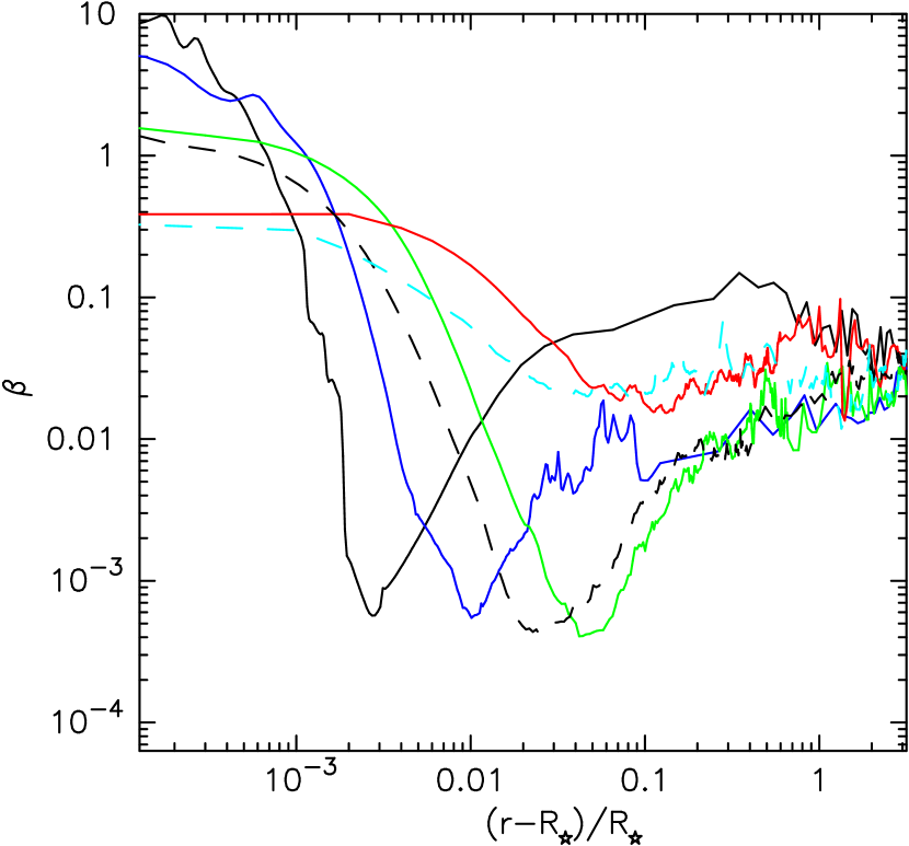
Figure 9: Plasma $\beta$ values as functions of stellar radii. The solid lines are the results of the $1M_{\odot}$ star; the black, blue, green, and red lines are the results of the star with the surface gravity, $\log g=4.4$ (Sun), 3.4, 2.4, and 1.4, respectively. The dashed lines are the results of the $3\;M_{\odot}$ stars; the black and light-blue lines are the results of the stars with the surface gravity, $\log g=2.4$ and 1.4.

The Alfvén wave-driven stellar wind plays an important role in terms of the energy conversion from magnetic energy to other types of energy. To study the energy conversion, a plasma $\beta$ value, which is defined as the ratio of gas pressure to magnetic pressure,

$$\beta=8\pi p/B^{2},$$ (9)

is a useful parameter. Figure 9 shows the $\beta$ values for the different six models. In the region closed to the surface, the $\beta$’s decrease on $r$ at first, which is more clearly seen in the unevolved stars. In this region, the atmosphere is mostly static and the density decreases rapidly according to an exponential manner. The decrease of the density is faster than the decrease of the magnetic energy $\propto B^{2}$, and then, the atmosphere becomes magnetically dominated, $\beta<1$. If the static atmosphere continued to the upper altitudes without the dissipation of the Alfvén waves, the $\beta$ values would keep decreasing.

In reality, however, the density structure is redistributed by the heating from the wave dissipation. In the main sequence ($\log g=4.4$) and subgiant ($\log g=3.4$) stars, the hot coronae are formed, which give larger pressure scale heights ( $\propto$ temperature). Therefore, the densities decrease more slowly than the magnetic energy, and the $\beta$ values increase in the coronal regions. In the red giant stars, although hot coronae do not form as in the main sequence and subgiant stars, the gas is lifted up directly by magnetic pressure associated with Alfvén waves in the weak gravity conditions, which are gradually connected to the stellar wind regions. Interestingly, the final $\beta$ values are $0.01-0.1$, being independent from the surface gravities. The redistribution of the density through the wave dissipation makes the plasma $\beta$ values stay at the moderate values.

4 Turbulent-driven Accretion Disk Winds

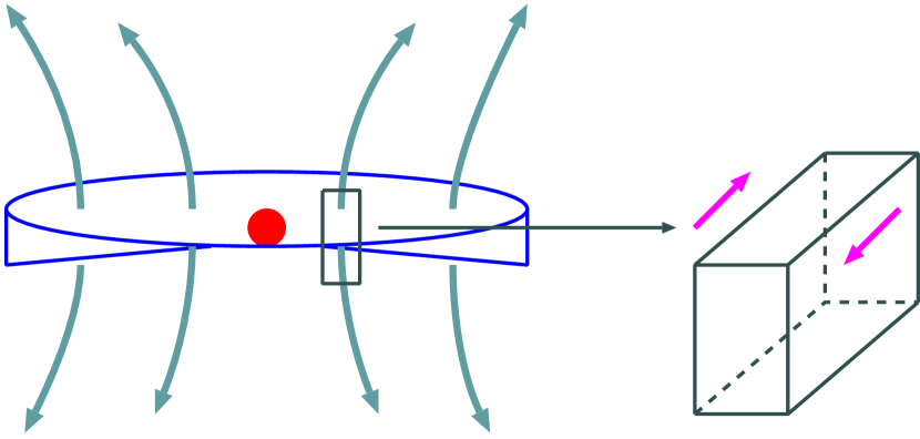
Figure 10: Schematic picture of the local shearing box simulation of an accretion disk.

We investigated accretion disk winds that are driven by MHD turbulence in accretion disks (Suzuki & Inutsuka, 2009). The geometrical aspects of disk winds are different from those of the stellar winds as easily expected. On the other hand, the driving mechanism shows similarities to the solar and red giant winds, which we discuss from now.

To study turbulence driven accretion disk winds, we performed 3D MHD simulations in a local patch of an accretion disk (Hawley et al. 1995; Matsumoto & Tajima 1995; Figure 10). Here, we neglect the effects of curvature and the simulations are carried out in a local Cartesian box that co-rotates with a Keplerian rotating disk. Following the convention (Hawley et al. 1995), $x$, $y$, and $z$ coordinates corresponds to radial, azimuthal, and vertical directions, respectively. While in the $x$ direction we do not take into account the radial gradients of the background density, in the $z$ direction the density stratification owing to the gravity by a central star is included. The size of the simulation box is $(x,y,z)=(\pm 0.5H,\pm 2H,\pm 4H)$, where a scale height, $H$, is defined from rotation frequency, $\Omega$, and sound speed as $H=\sqrt{2}c_{s}/\Omega$. We use $(32,64,256)$ mesh points for the $(x,y,z)$ coordinates. The $z$ size of the simulation box covers from the sufficiently lower region to upper region of an entire disk so that we can simultaneously treat the amplification of magnetic field by MRI and excitation of disk winds in a self-consistent manner. This is an advantage of the simulation of the accretion disk winds in comparison to the simulations of solar/stellar winds, in which we give the conditions at the surface based observationally inferred values without considering the generation of the magnetic field in the solar/stellar interiors.

Because the co-rotating box is not in an inertial coordinate, inertial forces need to be taken into account in the momentum equations :

$$\frac{d\mbox{\boldmath${v}$}}{dt}=-\frac{1}{\rho}\nabla(p+\frac{B^{2}}{8\pi})+\frac{(\mbox{\boldmath${B}$}\cdot\nabla)\mbox{\boldmath${B}$}}{4\pi\rho}-2\mbox{\boldmath${\Omega_{0}}$}\times\mbox{\boldmath${v}$}+3\Omega_{0}^{2}\mbox{\boldmath${x}$}-\Omega_{0}^{2}\mbox{\boldmath${z}$},$$ (10)

where the third term on the right hand side is Coriolis force, the fourth term corresponds to tidal expansion which is the sum of centrifugal force and the radial direction of the gravity by a central star, and the last term is the vertical component of the gravity which gives the stratification of the density in the vertical direction. We assume isothermal gas instead of solving the energy equation in order to focus of the dynamics of the disk winds. In the $x$ direction, the shearing boundary condition (Hawley et al.1995) is adopted to mimic the differential rotation of a Keplerian rotating disk. The simple periodic boundary condition is applied to the $y$ direction. The outgoing condition (SI06) is prescribed to the $z$ direction to properly treat streaming out disk winds. We would like to note that our simulation is the first attempt that adopts the real outgoing boundary to the disk wind simulation in the local shearing box, whereas the simple zero-gradient boundary was used in previous studies (Miller & Stone, 2000; Hirose et al., 2006). As the initial condition, we give Keplerian rotation, $v_{x}=-3/2\Omega x$, with small perturbations as seeds for MRI and set up weak vertical magnetic fields with $\beta=10^{6}$ at the midplane. In the vertical direction, we give the hydrostatic density structure, $\rho\propto\exp(-z^{2}/H^{2})$.

Figure 11: Time-averaged disk structure during $t=200-400$ rotations. The variables are also averaged on $x-y$ plane at each $z$ grid. The top left panel shows $v_{z}/c_{s}$ (solid), whereas the dotted line is the initial condition ($v_{z}/c_{s}=0$). The bottom left panel presents the density (solid) in comparison with the initial condition (dotted). The top right panel presents magnetic energy, $B^{2}/4\pi$. The dashed, solid, and dotted lines correspond to $x$, $y$, and $z$ components, whereas the $y$ component shows both mean (thick) and fluctuation (thin) components. The bottom right panel shows the plasma $\beta$ (solid) in comparison with the initial value (dotted).

In this review paper we mainly focus on the time-averaged structure of disk winds. We would like to briefly describe the time evolution and dynamical properties of the simulated local accretion disk (see Suzuki & Inutsuka 2009 for more detail). After $\sim 3$ rotations, MRI triggers MHD turbulence firstly around $z\sim\pm(2-3)H$. In the higher regions ($|z|>3H$), MRI does not set in because the circumstance is magnetically dominate from the beginning and stable against MRI. On the other hand, the delay of the MRI trigerring in the near-midplane region is an artifact. Since in this region the plasma $\beta$ is too high (gas pressure dominated) at first, we cannot resolve the most unstable wavelength of MRI. However, MRI gradually takes place later on. As the magnetic field strength increases, the most unstable wavelength can be eventually resolved at the midplane. After 100 rotation, the entire region except the surface regions ($|z|>3H$) becomes turbulent and the disk winds are driven by MHD turbulent pressure from the upper and lower surfaces. At $200$ rotations, the magnetic field strength almost saturates, balancing the amplification by MRI with the cancellation by magnetic reconnections and the escape with the disk winds. At this time, the magnetic energy is amplified 1000 times of the initial energy of the weak vertical field, and the field lines are dominated by the toroidal ($y$) component (see below).

An interesting feature is that the disk winds are blow off intermittently. The mass fluxes of the disk winds become strong every 5-10 rotations quasi-periodically. This is a consequence of breakups of large scale channel flows at $z\approx\pm 2H$ (Suzuki & Inutsuka 2009).

Figure 11 presents the disk wind structure averaging over 200 - 400 rotations. The variables are averaged on the $x-y$ plane at each $z$ point. The top left panel shows that the gas streams out of the upper and lower surfaces. The average outflow velocity is nearly the sound speed at the upper and lower boundaries. The disk winds are dominantly accelerated by magnetic energy (Poyinting flux) of the MHD turbulence, which we inspect from now.

The top right panel shows magnetic energy at the saturated state. The dashed, solid, and dotted lines are $x$, $y$, and $z$ components. In the $y$ component we are showing both mean, $\langle B_{y}\rangle^{2}$ and fluctuation, $\delta B_{y}^{2}$, components. $\langle B_{y}\rangle^{2}$ is the simple average on $x-y$ planes, $\langle B_{y}(z)\rangle=\int\int dxdyB_{y}(x,y,z)/(L_{x}L_{y})$, and the the fluctuations are determined from $\delta B_{y}^{2}(z)=\int\int dxdy(B_{y}(x,y,z)-\langle B_{y}(z)\rangle)^{2}/(L_{x}L_{y})$, where $L_{x}(=H)$ and $L_{y}(=4H)$ are the $x$ and $y$ lengths of the simulation box. As for $B_{x}$ and $B_{z}$ the fluctuation components greatly dominate the means, and so we simply present $B_{x}^{2}$ and $B_{z}^{2}$. The magnetic energy, which is dominated by the toroidal ($y$) component as a consequence of winding, is amplified by $\approx$ 1000 times of the initial value ($B_{z,0}^{2}/4\pi=10^{-6}$) in most of the region ($|z|<3H$). While in the region near the mid-plane ($|z|<1.5H$), the magnetic field is dominated by fluctuating component ($\delta B_{y}$), the coherent component ($\langle B_{y}\rangle$) dominates in the regions near the surfaces ($|z|>1.5H$). In the surface regions the magnetic pressure is comparable to or larger than the gas pressure ($\beta\;\buildrel<\over{\sim}\;1$), and thus, the gas motions cannot control the configuration of the magnetic fields. Therefore, the field lines tend to be straightened by magnetic tension to give $\langle B\rangle^{2}>\delta B^{2}$ there, even if the gas is turbulent. We also note that $\langle B_{z}^{2}\rangle$ is amplified by MRI and Parker (1966) instability, whereas $\langle B_{z}\rangle^{2}$ is strictly conserved.

The comparison of the final density structure (solid) with the initial hydrostatic structure (dotted) in the bottom left panel shows that the mass is loaded up to the onset regions of outflows from $z\approx\pm 2H$ by the amplified magnetic energy. The plasma $\beta$ value in the bottom right panel is a good indicator to understand the locations of the mass loading. The panel shows that the wind onset regions correspond to $\beta\approx 1$, which indicates that the winds start to be accelerated when the magnetic pressure exceeds the gas pressure. In the further upper regions, $|z|\;\buildrel>\over{\sim}\;3H$, $\beta$ stays almost constant slightly below unity. Without disk winds, $\beta$ decreases with increasing height in the hydrostatic structure. However, the mass loading and disk winds inhibit the decrease of $\beta$. We can interpret that the density structure is redistributed to give the almost constant $\beta$ in the wind regions. This is, in a qualitative sense, similar to the $\beta$ structures in the stellar winds (Figure 9). The detailed features are different mainly because we do not solve the energy equation with radiative cooling and conduction in the disk wind simulations.

Figure 12: Time-averaged Poynting associated magnetic tension, $-B_{z}v_{\perp}B_{\perp}$, flux of magnetic tension.

The disk winds are driven by Poynting flux; both magnetic pressures and tension almost equally contribute. The magnetic tension term, $-B_{z}v_{\perp}B_{\perp}$ ($\perp$ denotes $x$ and $y$) shows an interesting distribution, which is shown in Figure 12. In the surface regions, the absolute values decrease with increasing $z$, because the Poynting flux is converted to the kinetic energy of the disk winds; this is natural behavior. However, at $|z|\approx\pm 1.5H$, the solid line crosses the 0 line. This indicates that the Poynting flux of the tension force directs toward both surface and midplane from here. This is a result of the breakups of large scale channel flows at $|z|\approx\pm 1.5H$ (Suzuki & Inutsuka, 2009).

The Poynting flux associated with Alfvén waves is expressed as the same shape, $-B_{z}v_{\perp}B_{\perp}$, because they are propagating by tension restoring force. The properties of the Poynting flux of the magnetic tension shown in Figure 12 are different from the Alfvén waves discussed in the solar and stellar winds, because $\delta B_{\perp}\gg B_{z}$ in the disk wind situation. The Poynting flux here is mainly by large-scale channel flows in mid altitude regions ($z\sim 2H$) and is associated with a U-shape magnetic field by Parker instability in the surface regions ($|z|\;\buildrel>\over{\sim}\;3H$: Suzuki et al.2010).

5 Summary

We have introduced the results of our simulation studies on Alfvén wave-driven winds. In the section 2 we summarized the solar wind simulations presented in SI05 and SI06, emphasizing the reflection of Alfvén waves. In the standard run, 15% of the initial wave energy flux from the photosphere can transmit into the corona, which is sufficient for the heating and acceleration of the solar winds. The Alfvén waves nonlinearly generate compressive waves which eventually steepen and heat up the ambient gas by the shock heating. In another way of the explanation, the outgoing Alfvén waves dissipate by parametric decay to incoming Alfvén waves and outgoing compressive waves. This process is very efficient in the density stratified atmosphere.

The structure of the solar winds shows very sensitive dependence on the input wave amplitude by the positive feedback mechanism: When increasing the amplitude, the coronal density becomes larger and the pressure scale height becomes longer because of the larger heating. The larger density enhances the wave dissipation because the wave nonlinearly is larger owing to the smaller Alfvén speed ($\propto 1/\sqrt{\rho}$). The longer pressure scale height reduces the wave reflection. Therefore, the heating is enhanced when the surface amplitude slightly increases. This shows that the structure of solar wind is largely altered on a small change of the input energy through the reflection and the nonlinear dissipation of the Alfvén waves.

We introduced recent HINODE observations of Alfvénic oscillations. The obtained data by Fujimura & Tsuneta (2009) can be explained by the sum of upgoing Alfvén waves and the comparable amount of the reflected component. They can estimate the leakage Poynting flux of the Alfvénic oscillations to the upper location from the phase correlation of the perturbing magnetic field and the velocity. They analyzed one case and found that the sufficient energy to heat the corona and solar wind is going upward. These observed properties are quite consistent with what we get in the simulations.

We discussed the roles of Alfvén waves in the context of stellar evolution. Before reaching AGB phase when dusts are formed in cool atmosphere, it is expected that, similarly to the solar wind, the Alfvén waves play a major role in driving the stellar winds. By using the surface fluctuation strength estimated from the convective flux, we performed the MHD simulations. When a star evolves to RGB phase, the hot corona suddenly disappears and the atmosphere streams out as the cool chromospheric winds in which magnetized hot bubbles intermittently float. The main reason of the disappearance of the hot corona is the gravity effect; the atmosphere flows out before heated up owing to the weak gravity confinement. In addition, the thermal instability also plays a role in the sudden drop of the temperature. In evolved stars, the Alfvén waves do not suffer reflection because the density decreases more slowly and the change of Alfvén speeds become more gradual. This is a part of the reason why the mass loss rate jumps up with stellar evolution.

We also introduced the accretion disk winds by MHD turbulence amplified by MRI. The disk winds are driven by Poynting flux when the magnetic energy dominates the gas energy. In the disk wind regions the plasma $\beta$ value is kept slightly below unity by the redistribution of the density structure, which is qualitatively similar to what we got in the simulation of the solar and stellar winds. On the other hands, the disk winds are intermittent mainly because of the breakups of large scale channel flows. In the simulations, we only model the onset region of the disk winds. In further upper region with magnetically dominated condition, Alfvén waves might play a role in accerating the winds.