Vibrational Tamm states at the edges of graphene nanoribbons

Abstract

We study vibrational states localized at the edges of graphene nanoribbons. Such surface oscillations can be considered as a phonon analog of Tamm states well known in the electronic theory. We consider both armchair and zigzag graphene stripes and demonstrate that surface modes correspond to phonons localized at the edges of the graphene nanoribbon, and they can be classified as in-plane and out-of-plane modes. In addition, in armchair nanoribbons anharmonic edge modes can experience longitudinal localization in the form of self-localized nonlinear modes, or surface breather solitons.

I Introduction

Graphite nanocrystallites are recently discovered carbon-based nanomaterials p1 which are a few atoms thick and stable under ambient conditions, and they keep many promises as materials for nanoscale transistors p2 . Remarkable properties of graphite structures make their study one of the hot topics of nanoscience p3 .

Graphene nanoribbons are effectively low-dimensional nanostructures similar to carbon nanotubes, but they differ from nanotubes by the presence of edges. Due to the edges, graphene nanoribbons can demonstrate many novel geometry-driven properties, depending on their width and helicity. A majority of the current studies of graphene nanoribbons target their electronic and magnetic properties stipulated by the presence of edges, including the existence of the edge modes lee , which are an analog of surface states in this two-dimensional geometry.

In general, surface states are spatially localized modes which can be generated at surfaces book_S , and such surface states have been studied in many branches of of physics including electrons in crystals Tamm ; Shockley , surface phonons Maradudin , surface polaritons Agranovich , and optical surface modes in waveguide arrays ivan ; ivan_exp . In this paper, we analyze the specific properties of vibrational phonon modes localized at the edges of graphene nanoribbons, the so-called edge phonon modes. Such localized surface modes can be considered as a phonon analog of Tamm states well known in the electronic theory Tamm .

Vibrational edge modes in graphene nanoribbons have been discussed recently for the hydrogen-terminated graphene nanoribbons p4 . Using the second-generation reactive empirical bond-order potential and density-functional theory calculations, it was demonstrated that two different edge modes can exist in armchair nanoribbons, whereas the zigzag nanoribbons can support only one such mode. Importantly, all those edge modes were found to correspond to the out-of-plane vibrations of the edge hydrogen atoms.

In this paper, we employ numerical analysis and molecular dynamics simulations to study localized modes in graphene nanoribbons. We demonstrate that such nanostructures can support much larger number of vibrational phonon modes localized at the edges. More specifically, we find that the armchair nanoribbon can support 7 edge modes, whereas the zigzag nanoribbon can support 12 edge modes. Only one part of such modes correspond to out-of-plane oscillations of the edge atoms, whereas and the second part is characterized by in-plane edge oscillations. Chemical modification of the edge atoms can lead to the generation of larger number of localized surface modes. In addition, numerical simulations of anharmonic oscillations demonstrate that in armchair nanoribbons the vibrational energy can become self-trapped along the edge of the stripe with the formation of both in-plane and out-of-plane surface breather solitons.

The paper is organized as follows. In Sec. II we discuss our model including the potentials for describing the interatomic interactions and the edge effects. Section III is devoted to a general linear analysis, and it discusses the dispersion curves for both armchair and zigzag nanoribbons. In Sec. IV we describe the specific properties of the edge modes and corresponding energy localization. Some properties of anharmonic oscillations and surface breather solitons are discussed in Sec. V, whereas Sec. VI concludes the paper.

II Model of graphene nanoribbons

We model the graphene nanoribbon as a planar stripe of graphite, with the properties depending on the stripe width and chirality. Here we consider two most typical geometries of the armchair nanoribbon [see Fig. 1(a)] and zigzag nanoribbon [see Fig. 1(b)].

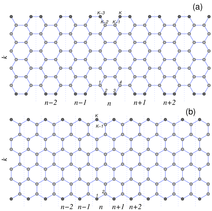
Figure 1: Schematic view of (a) armchair and (b) zigzag nanoribbons with the atom numbering. The edge atoms are shown as filled circles. Dotted lines separate the elementary cells of the nanoribbon. $M$ is the number of atoms in the elementary cell.

The structure of the nanoribbon can be presented through a longitudinal repetition of the elementary cell composed of $K$ atoms, as shown in Figs. 1(a,b). For the armchair, the number $K$ is multiple of 4, whereas for the zigzag nanoribbon the number $K$ is multiple of 2. We use the atom numbering shown in Figs. 1(a,b). In this case, each carbon atom has a two-component index $\alpha=(n,k)$, where $n=0,\pm 1,\pm 2,...$ stands for the number of the elementary cells, and $k=1,2,...,K$ stands for the number of atoms in the cell.

Each elementary cell of the armchair nanoribbon has four edge atoms, whereas the zigzag nanoribbon has only two edge atoms. In Figures 1(a,b), we show these edge atoms as filled circles. In a realistic case, the edge atoms are chemically modified and, generally speaking, the following situations are possible p5 ; p6 : a single hydrogen CH (hydrogen-terminated graphene nanoribbon), CH₂ – two hydrogens, COH – a hydroxyl group, and CHOH – a hydrogen atom and a hydroxyl group that resulted from the water decomposition.

In this study, we do not take into account the specific chemical nature of the surface atoms, but consider a change of the effective mass of the edge atom. Therefore, in our model of graphene nanoribbons we take the mass of atoms inside the stripe as $M_{0}=12m_{p}$, and for the edge atoms we consider a larger mass, such as $M_{1}=13m_{p}$, $14m_{p}$, $29m_{p}$, $30m_{p}$ (where $m_{p}=1.6603\cdot 10^{-27}$kg is the proton mass).

To describe nanoribbon oscillations, we write the system Hamiltonian in the form,

$$H=\sum_{n=-\infty}^{+\infty}\sum_{k=1}^{K}\left[\frac{1}{2}M_{(n,k)}(\dot{\bf u}_{(n,k)},\dot{\bf u}_{(n,k)})+P_{(n,k)}\right],$$ (1)

where $M_{\alpha}$ is the mass of the hydrogen atom with the index $\alpha=(n,k)$ (for internal atoms we take $M_{\alpha}=M_{0}$, whereas for the edge atoms we take a larger mass, $M_{\alpha}=M_{1}>M_{0}$), ${\bf u}_{\alpha}=(x_{\alpha}(t),y_{\alpha}(t),z_{\alpha}(t))$ is the radius-vector of the carbon atom with the index $\alpha$ at the moment $t$. The term $P_{\alpha}$ describes the interaction of the atom with the index $\alpha=(n,k)$ and its neighboring atoms. The potential depends on variations of bond length, bond angles, and dihedral angles between the planes formed by three neighboring carbon atoms, and it can be written in the form

$$P=\sum_{\Omega_{1}}U_{1}+\sum_{\Omega_{2}}U_{2}+\sum_{\Omega_{3}}U_{3}+\sum_{\Omega_{4}}U_{4}+\sum_{\Omega_{5}}U_{5},$$ (2)

where $\Omega_{i}$, with $i=1,2,3,4,5$, are the sets of configurations including up to nearest-neighbor interactions. Owing to a large redundancy, the sets only need to contain configurations of the atoms shown in Fig. 2, including their rotated and mirrored versions.

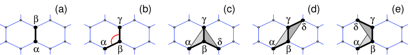
Figure 2: Configurations containing up to $i$-th nearest-neighbor interactions for: (a) $i=1$, (b) $i=2$, (c) $i=3$, (d) $i=4$, and (e) $i=5$.

The potential $U_{1}({\bf u}_{\alpha},{\bf u}_{\beta})$ describes the deformation energy due to a direct interaction between pairs of atoms with the indexes $\alpha$ and $\beta$, as shown in Fig. 2(a). The potential $U_{2}({\bf u}_{\alpha},{\bf u}_{\beta},{\bf u}_{\gamma})$ describes the deformation energy of the angle between the valent bonds ${\bf u}_{\alpha}{\bf u}_{\beta}$ and ${\bf u}_{\beta}{\bf u}_{\gamma}$, see Fig. 2(b). Potentials $U_{i}({\bf u}_{\alpha},{\bf u}_{\beta},{\bf u}_{\gamma},{\bf u}_{\delta})$, $i=3$, 4, 5, describes the deformation energy associated with a change of the effective angle between the planes ${\bf u}_{\alpha},{\bf u}_{\beta},{\bf u}_{\gamma}$ and ${\bf u}_{\beta},{\bf u}_{\gamma},{\bf u}_{\delta}$, as shown in Figs. 2(c,d,e).

We use the potentials employed in the modeling of the dynamics of large polymer macromolecules p7 ; p8 ; p9 ; p10 ; p11 for the valent bond coupling,

$$U_{1}({\bf u}_{1},{\bf u}_{2})=\epsilon_{1}\{\exp[-\alpha_{0}(\rho-\rho_{0})]-1\}^{2},~{}~{}~{}\rho=|{\bf u}_{2}-{\bf u}_{1}|,$$ (3)

where $\epsilon_{1}=4.9632$ eV is the energy of the valent bond and $\rho_{0}=1.418$ Å  is the equilibrium length of the bond; the potential of the valent angle

$$U_{2}({\bf u}_{1},{\bf u}_{2},{\bf u}_{3})=\epsilon_{2}(\cos\varphi-\cos\varphi_{0})^{2},$$ (4)

$$\cos\varphi=({\bf u}_{3}-{\bf u}_{2},{\bf u}_{1}-{\bf u}_{2})/(|{\bf u}_{3}-{\bf u}_{2}|\cdot|{\bf u}_{2}-{\bf u}_{1}|),$$

so that the equilibrium value of the angle is defined as $\cos\varphi_{0}=\cos(2\pi/3)=-1/2$; the potential of the torsion angle

$$U_{i}({\bf u}_{1},{\bf u}_{2},{\bf u}_{3},{\bf u}_{4})=\epsilon_{i}(1-z_{i}\cos\phi),$$ (5)

$$\cos\phi=({\bf v}_{1},{\bf v}_{2})/(|{\bf v}_{1}|\cdot|{\bf v}_{2}|),$$

$${\bf v}_{1}=({\bf u}_{2}-{\bf u}_{1})\times({\bf u}_{3}-{\bf u}_{2}),$$

$${\bf v}_{2}=({\bf u}_{3}-{\bf u}_{2})\times({\bf u}_{3}-{\bf u}_{4}),$$

where the sign $z_{i}=1$ for the indices $i=3,4$ (equilibrium value of the torsional angle $\phi_{0}=0$) and $z_{i}=-1$ for the index $i=5$ ($\phi_{0}=\pi$).

The specific values of the parameters are $\alpha_{0}=1.7889$ Å^-1, $\epsilon_{2}=1.3143$ eV, and $\epsilon_{3}=0.499$ eV, and they are found from the frequency spectrum of small-amplitude oscillations of a sheet of graphite p12 . According to the results of Ref. p13 the energy $\epsilon_{4}$ is close to the energy $\epsilon_{3}$, whereas $\epsilon_{5}\ll\epsilon_{4}$ ($|\epsilon_{5}/\epsilon_{4}|<1/20$). Therefore, in what follows we use the values $\epsilon_{4}=\epsilon_{3}=0.499$ eV and assume $\epsilon_{5}=0$, the latter means that we omit the last term in the sum (2).

III Dispersion curves

In the equilibrium state, $\{{\bf u}^{0}_{(n,k)}\}_{n=-\infty,~{}k=1}^{+\infty,~{}K}$, all atoms are in the plane of the nanoribbon, so that all valent bonds have the equilibrium length $\rho=\rho_{0}$, and all angle between the bonds coincide, $\varphi=2\pi/3$. Armchair nanoribbon is characterized by the longitudinal shift $h_{x}=3\rho_{0}$ and width $D_{y}=\sqrt{3}(K/2-1)\rho_{0}/2$, where $K$ is the number of atoms in the elementary cell. Zigzag nanoribbon is characterized by the longitudinal shift $h_{x}=\sqrt{3}\rho_{0}$ and width $D_{y}=\rho_{0}(3K-4)/4$.

Next, we introduce $3K$-dimensional vector,

$${\bf x_{n}}=({\bf u}_{(n,1)}-{\bf u}^{0}_{(n,1)},...,{\bf u}_{(n,K)}-{\bf u}^{0}_{(n,K)})$$

describing a shift of the atom of the $n$-th cell from its equilibrium position. Then, the nanoribbon Hamiltonian can be written in the following form,

$$H=\sum_{n}\{\frac{1}{2}({\bf M}\dot{\bf x}_{n},\dot{\bf x}_{n})+{\cal P}({\bf x}_{n-1},{\bf x}_{n},{\bf x}_{n+1})\},$$ (6)

where ${\bf M}$ is the diagonal matrix of masses of all atoms of the elementary cell.

Hamiltonian (6) generates the following set of the equations of motion:

$$-{\bf M}\ddot{\bf x}_{n} = {\cal P}_{{\bf x}_{1}}({\bf x}_{n},{\bf x}_{n+1},{\bf x}_{n+2})+{\cal P}_{{\bf x}_{2}}({\bf x}_{n-1},{\bf x}_{n},{\bf x}_{n+1})$$ (7)

$$+{\cal P}_{{\bf x}_{3}}({\bf x}_{n-2},{\bf x}_{n-1},{\bf x}_{n})$$

In the linear approximation, this system takes the form

$$-{\bf M}\ddot{\bf x}_{n}={\bf B}_{1}{\bf x}_{n}+{\bf B}_{2}{\bf x}_{n+1}+{\bf B}^{*}_{2}{\bf x}_{n-1}+{\bf B}_{3}{\bf x}_{n+2}+{\bf B}^{*}_{3}{\bf x}_{n-2},$$ (8)

where the matrix elements are defined as

$${\bf B}_{1}={\cal P}_{{\bf x}_{1}{\bf x}_{1}}+{\cal P}_{{\bf x}_{2}{\bf x}_{2}}+{\cal P}_{{\bf x}_{3}{\bf x}_{3}},$$

$${\bf B}_{2}={\cal P}_{{\bf x}_{1}{\bf x}_{2}}+{\cal P}_{{\bf x}_{2}{\bf x}_{3}},~{}{\bf B}_{3}={\cal P}_{{\bf x}_{1}{\bf x}_{3}},$$

and the matrix of the partial derivatives takes the form

$${\cal P}_{{\bf x}_{i}{\bf x}_{j}}=\frac{\partial^{2}\cal P}{\partial{\bf x}_{i}\partial{\bf x}_{j}}({\bf 0},{\bf 0},{\bf 0}),~{}~{}i,j=1,2,3.$$

Solutions of the system of linear equations (8) can be sought in the standard form,

$${\bf x}_{n}=A{\bf e}\exp(iqn-i\omega t),$$ (9)

where $A$ is the mode amplitude, ${\bf e}$ is the normalized dimensionless vector ($({\bf Me},{\bf e})/M_{0}=1)$, $q\in[0,\pi]$ is the dimensionless wave number, and $\omega$ is the phonon frequency. Substituting the expression (9) into the system (8), we obtain the eigenvalue problem

$$\omega^{2}{\bf Me}=[{\bf B}_{1}+{\bf B}_{2}e^{iq}+{\bf B}_{2}^{*}e^{-iq}+{\bf B}_{3}e^{2iq}+{\bf B}_{3}^{*}e^{-2iq}]{\bf e}.$$ (10)

Therefore, in order to find the dispersion relations characterizing the modes of the nanoribbon for each fixed value of the wave number $0\leq q\leq\pi$ we need to find the eigenvalues of the Hermitian matrix (10) of the order $3K\times 3K$. As a result, the dispersion curves are composed of $3K$ branches $\{\omega_{j}(q)\}_{j=1}^{3K}$, as shown in Fig. 3. Two thirds of the branches corresponds to the atom vibrations in the plane of the nanoribbon $xy$ (in-plane vibrations), whereas only one third corresponds to the vibrations orthogonal to the plane (out-of-plane vibrations), when the atoms are shifted along the axes $z$.

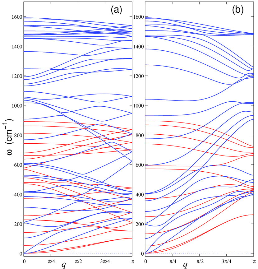
Figure 3: (color online) Structure of $3K$ dispersion curves for (a) armchair nanoribbon with the width $D_{y}=11.05$ Å  ($K=20$), and (b) zigzag nanoribbon with the width $D_{y}=11.34$ Å  ($K=12$). Blue (black) curves correspond to the in-plane vibrations, and red (gray) curves correspond to out-of-plane vibrations. Mass of the edge atoms is $M_{1}=13m_{p}$.

As is seen in Fig. 3, the spectrum of the nanoribbon oscillations occupies the frequency interval $[0,\omega_{m}]$, where the maximum (cutoff) frequency $\omega_{m}$ practically does not depend on the chirality. The maximum frequency $\omega_{m}=1600$ cm^-1. This value agrees well with the experimental data for a planar graphite p14 ; p15 . Four branches of the dispersion curves start from the origin, $(q=0,~{}\omega=0)$. The first branch $\omega_{1}(q)$ corresponds to the orthogonal (out-of-plane) bending vibrations of the nanoribbon; the second branch $\omega_{2}(q)$ describes the bending planar (in-plane) vibrations in the plane. These branches approach smoothly the axes $q$: $\omega(q)/q\rightarrow 0$, when $q\rightarrow 0$, so that the corresponding long-wave phonons possess no dispersion. The third $\omega_{3}(q)$ and fourth $\omega_{4}(q)$ branches of the dispersion curves correspond to the out-of-plane twisting and in-plane longitudinal vibrational modes, respectively. The corresponding long-wave modes possess nonzero dispersion, so that we can define two limiting values,

$$v_{t}=h_{x}\lim_{q\rightarrow 0}\frac{\omega_{3}(q)}{q},~{}~{}\mbox{and}~{}~{}v_{l}=h_{x}\lim_{q\rightarrow 0}\frac{\omega_{4}(q)}{q}$$

which defines the sound speeds of twisting and longitudinal phonons in the nanoribbon. The values of these speeds depend on the nanoribbon chirality. Nanoribbons of the same width but different chiralities support phonons with different sound speeds: armchair nanoribbon with $K=20$ (width $D_{y}=11.05$ Å) has the velocities $v_{t}=3400$ m/s and $v_{l}=24900$ m/s, whereas for the zigzag nanoribbon with $K=12$ (width $D_{y}=11.34$ Å) these velocities are smaller, $v_{t}=1900$ m/s and $v_{l}=13200$ m/s. When the width of the nanoribbon grows, the velocity of the longitudinal sound remains unchanged while the velocity of the twisting modes decreases monotonically.

IV Edge modes

Solution of the eigenvalue problem (10) demonstrates that the nanoribbon can support vibrational modes localized at the edges, the so-called edge phonons. To find such surface modes, we should consider the nanoribbons of a sufficiently large width, and we take the large number of atoms in the elementary cell, $K=120$.

To analyze oscillations (9), we define the distribution function of the oscillatory energy in the elementary cell of the nanoribbon as follows

$$p_{i}=M_{i}(|e_{3(i-1)+1}|^{2}+|e_{3(i-1)+2}|^{2}+|e_{3(i-1)+3}|^{2})/M_{0}\geq 0,$$

where $i=1,2,...,K$ is the number of atoms in the cell, $M_{i}$ is the mass of the $i$-th atoms, $e_{j}$ is the component of the eigenvector ${\bf e}=\{e_{j}\}_{j=1}^{3K}$. The energy distribution is normalized by the following condition,

$$\sum_{i=1}^{K}p_{i}=({\bf Me},{\bf e})/M_{0}=1.$$

We introduce the parameter characterizing the transverse energy localization in the nanoribbon as follows,

$$d=1/\sum_{i=1}^{K}p_{i}^{2}.$$

This parameter characterizes the inverse width of the energy localization in the elementary cell. If the vibrational mode is localized only on one atom (i.e. there exists an atom $i_{0}$ for which $p_{i_{0}}=1$), the inverse width is $d=1$. In the opposite limit, when the vibrational energy is distributed equally on all atoms ($p_{i}\equiv 1/K$), we have $d=K$, so that in a general case $1\leq d\leq K$.

To be more specific, we define the vibrational mode as being localized provided $d<20$. Our numerical analysis of the oscillatory eigenmodes shows that localization may occur only at the edges of the nanoribbon. The structure of the $3K$ dispersion curves of the armchair and zigzag nanoribbons are shown in Figs. 4 and 5, where thick lines mark the edge modes of the nanoribbon. Such localized surface modes exist in both armchair and zigzag nanoribbons.

Table 1: Frequencies $\omega$ (dimension $[\omega]=$cm^-1) of the localized edge oscillations with the wave numbers $q=0$ and $q=\pi$, depending on the nanoribbon chirality and mass of the edge atom $M_{1}$ (dimension $[M_{1}]=m_{p}$). Out-of-plane vibrations are marked by italic. Oscillations with the wave number $q=0$ are underlined. Corresponding energy densities of the edge modes are presented in Figs. 6 and 7.

type	$M_{1}$	1	2	3	4	5	6	7	8	9	10	11	12	13	14
armchair	13	227	1452	102	150	236	268	1067	-	-	-	-	-	-	-
armchair	30	151	303	971	1335	70	110	180	180	210	245	598	690	1113	1482
zigzag	13	583	1466	261	393	406	431	432	661	716	912	1194	1478	-	-
zigzag	30	547	1276	172	284	368	413	432	661	716	742	1136	1159	1455	-

Now we consider in more details the edge modes with the wave numbers $q=0$ and $q=\pi$. The values of the frequencies of these modes are summarized in Table 1. When the mass of the edge atom is $M_{1}=13m_{p}$ (the effective edge atom corresponds to the molecular group CH), the armchair nanoribbon has 7 edge modes (3 out-of-plane and 4 in-plane), and zigzag nanoribbon has 12 edge modes (6 out-of-plane and 6 in-plane). If the mass of the edge atoms is increased, the number of localized modes growths as well. For example, for $M_{1}=30m_{p}$ (when the effective edge atom corresponds to the molecular group CHOH), the armchair has already 14 edge modes (4 out-of-plane and 10 in-plane), and the zigzag nanoribbon has 13 edge modes (6 out-of-plane and 7 in-plane).

We notice that for $K=120$, an increase of the mass of the edge atoms does not change substantially the dispersion curves because the number of the edge atoms is much smaller than the number of atoms in the elementary cell (elementary cell of the armchair nanoribbon has 4 edge atoms, and the zigzag nanoribbon – 2 edge atoms). However, the surface modes are localized at the edge atoms, so that a change of the mass of the edge atoms change the mode frequency substantially. As can be seen from Figs. 4 and 5, a change of the mass of the edge atoms from $M_{1}=13m_{p}$ to $M_{1}=30m_{p}$ leads mainly to a shift of the dispersion curves corresponding to the edge modes. This behavior provides an additional indication of the existence of strongly localized surface modes with the properties different from those of the bulk modes.

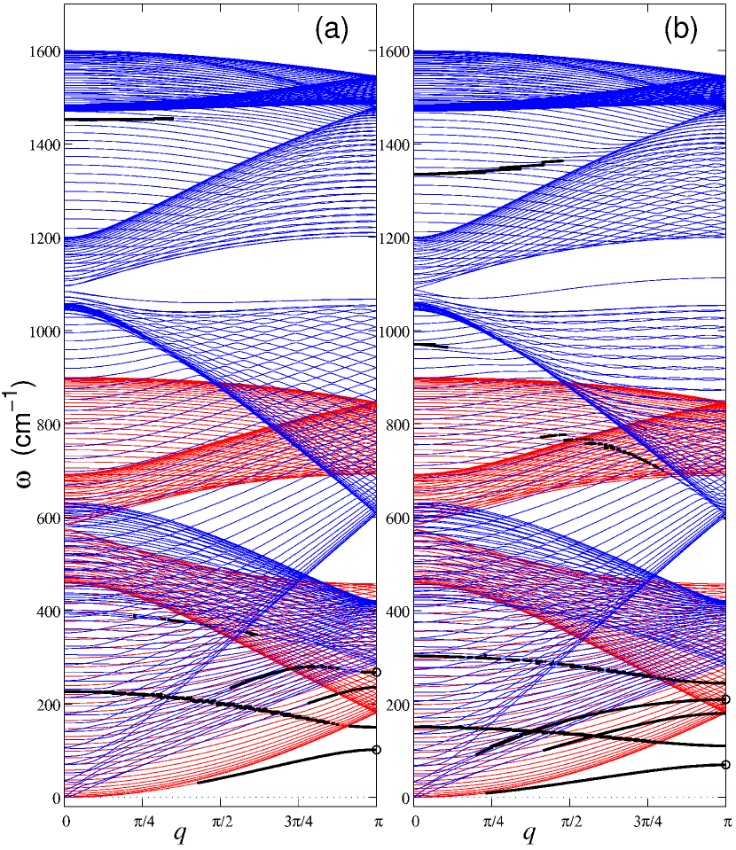
Figure 4: (color online) Structure of $3K$ dispersion curves of the armchair nanoribbons for (a) mass of the edge atoms $M_{1}=13m_{p}$ and (b) $M_{1}=30m_{p}$. The number of atoms in the elementary cell is $K=120$. Blue (black) curves correspond to in-plane vibrations, red (gray) curves – to the out-of-plane vibrations, thick black curves – oscillations localized at the nanoribbon edges. The marked points show the band edges where nonlinear breathers can appear in the form of the longitudinally localized edge modes.

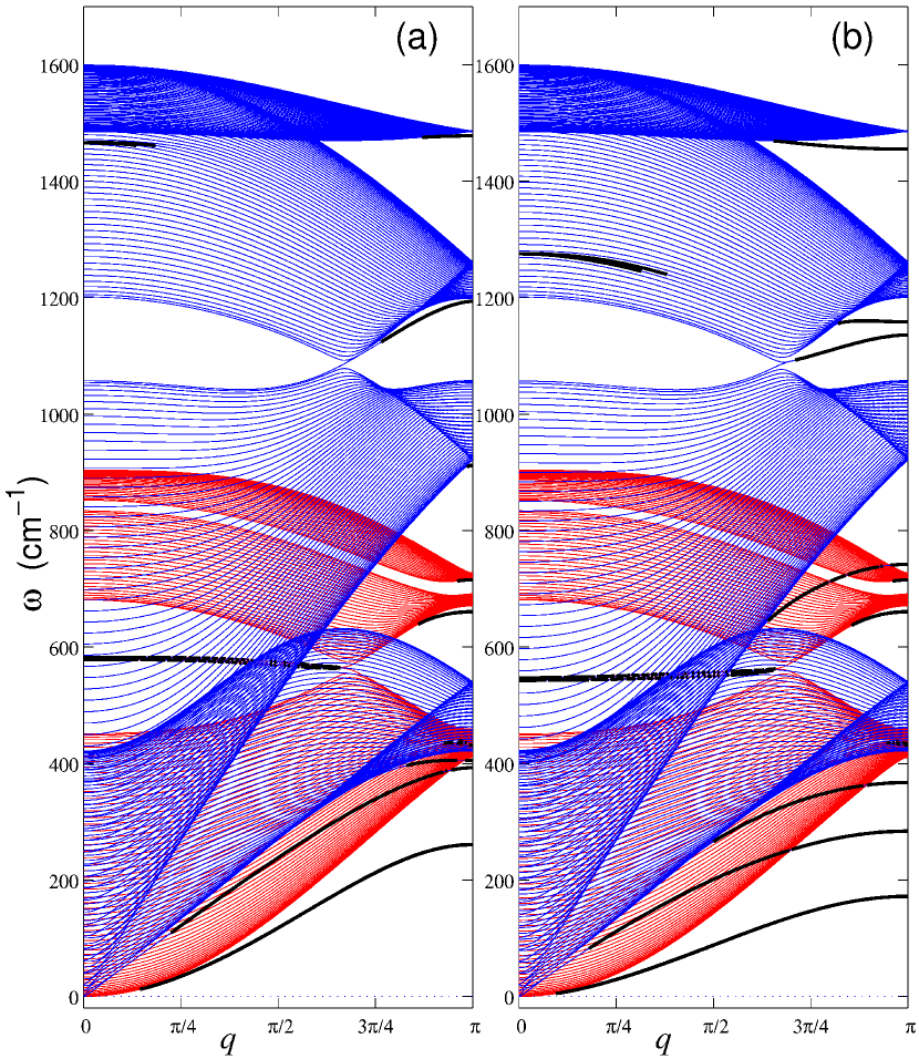
Figure 5: (color online) Structure of $3K$ dispersion curves of the zigzag nanoribbons for (a) mass of the edge atoms $M_{1}=13m_{p}$ and (b) $M_{1}=30m_{p}$. The number of atoms in the elementary cell is $K=120$. Blue (black) curves correspond to in-plane vibrations, red (gray) curves – to the out-of-plane vibrations, thick black curves – oscillations localized at the nanoribbon edges.

Transverse distribution of the energy of the surface localized states in the graphene nanoribbon is shown in Figs. 6 and 7. As follows from these results, the oscillations are mainly localized near the nanoribbon edges. For the armchair nanoribbon, the oscillations penetrate inside the stripe for less than 4 nm, and for the zigzag nanoribbon the oscillations decay for no more than 2 nm. For $M_{1}=13m_{p}$, the edge atoms of the armchair nanoribbon always participate in the surface vibration, whereas in zigzag nanoribbons the edge atoms may not contribute into the oscillatory mode, as shown in Fig. 7 for the modes with the numbers $l=6$, 7, 8 9).

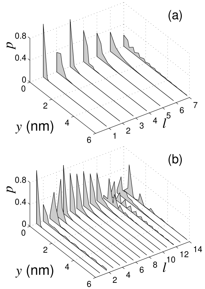
Figure 6: Transverse distribution of energy of the edge modes in the armchair nanoribbon with the wave numbers $q=0$, and $q=\pi$ for the mass of the edge atoms: (a) $M_{1}=13m_{p}$ ($q=0$ for $l\leq 2$, $q=\pi$ for $l\geq 3$) and (b) $M_{1}=30m_{p}$ ($q=0$ for $l\leq 4$, $q=\pi$ for $l\geq 5$). Here $y$ is the distance to the edge of the nanoribbon, $l$ is the mode number, $p(y)$ is the energy density normalized by the condition: $\int_{0}^{\infty}p(y)dy=1$. The values of the frequencies are summarized in Table 1.

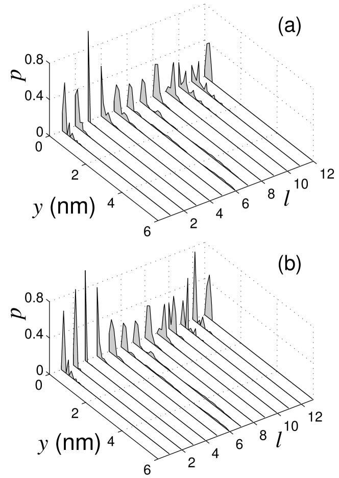
Figure 7: Transverse distribution of energy of the edge modes in the zigzag nanoribbon with the wave numbers $q=0$, and $q=\pi$ for the mass of the edge atoms: (a) $M_{1}=13m_{p}$ and (b) $M_{1}=30m_{p}$ ($q=0$ for $l\leq 2$, $q=\pi$ for $l\geq 3$). Here $y$ is the distance to the edge of the nanoribbon, $l$ is the mode number, $p(y)$ is the energy density normalized by the condition: $\int_{0}^{\infty}p(y)dy=1$. The values of the frequencies are summarized in Table 1.

The specific structure of the edge oscillations in the graphene nanoribbon are shown in Figs. 8 and 9. These edge modes can be divided into three groups. The first group is composed by low-frequency out-of-plane vibrations which mainly occur due to deformation of the soft dihedral angles. For the armchair nanoribbon with the mass of the edge atoms $M_{1}=13m_{p}$, these oscillations have the frequencies $\omega=102$, 150 and 227 cm^-1, whereas for the zigzag nanoribbons the similar modes have the frequencies: $\omega=261$, 431, 432, 583, 661, and 716 cm^-1. As can be seen from Figs. 6(a), 7(a), and Table 1, these oscillations are the most localized. The main vibrational energy is concentrated in the edge atoms, which oscillate orthogonally to the nanoribbon plane, except the modes in the zigzag nanoribbon with the frequencies 431, 432, 661, and 716 cm^-1 (here the edge atoms are static while the hexagons which contains these atoms rotate).

The second group of the edge modes is composed by the edge in-plane vibrations which occur due to a deformation of the valent angles. For the armchair nanoribbon these modes have the frequencies 236 and 268 cm^-1, and for the zigzag nanoribbon, the frequencies 393 and 406 cm^-1.

Finally, the third group of the surface modes is composed by high-frequency edge oscillations which occur in the nanoribbon plane which occur due to the deformation of the hard valent bonds. For the armchair nanoribbons, these are the edge modes with the frequencies 1067 and 1452 cm^-1, and for the zigzag nanoribbon, with the frequencies 912, 1194, 1466, and 1478 cm^-1.

We would like to mention that in the paper p4 the edge vibrations were studied by another method by using the second-generation reactive empirical bond order (REBOII) potential and density-functional theory calculations. This method does not allow to study nanoribbons of large width so that the authors of Ref. p4 considered the nanoribbons with $K=20$ atoms of hydrogen in the elementary cell, taking into account only the oscillations of the C–H groups. They found several types of the out-of-plane edge vibrational modes: two edge modes for the armchair nanoribbon (with the frequencies 365 and 858 cm^-1), and one mode for the zigzag nanoribbon (with the frequency 610 cm^-1).

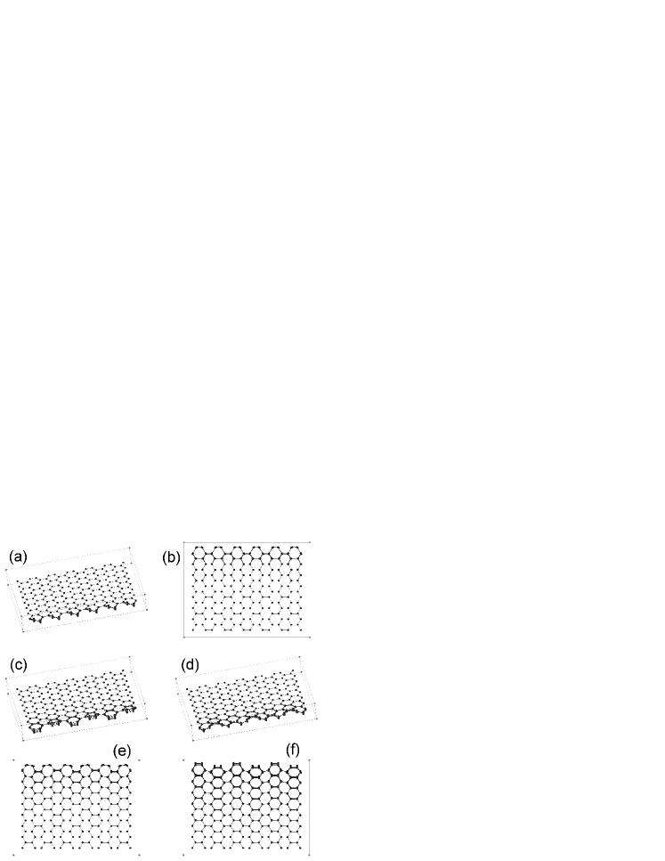
Figure 8: Six edge modes of the armchair nanoribbon. Shown are the displacements of atoms of the nanoribbon at quarter of an oscillation period, for: (a) out-of-plane vibration with $\omega=227$ cm^-1, $q=0$; (b) in-plane vibration with $\omega=1452$ cm^-1, $q=0$; (c) out-of-plane vibration with $\omega=102$ cm^-1, $q=\pi$; (d) out-of-plane vibration with $\omega=150$ cm^-1, $q=\pi$; (e) in-plane vibration with $\omega=236$ cm^-1, $q=\pi$; (f) in-plane vibration with $\omega=268$ cm^-1, $q=\pi$. Mass of the edge atom is $M_{1}=13m_{p}$.

In our work, using the mechanical model and direct molecular-dynamics numerical simulations allow to study much wider nanoribbons and, therefore, to find many more types of surface modes. We consider the edge C–H atomic group as a single edge atom with the mass $M_{1}=13m_{p}$, so that we are not able to study the vibrational mode associated with the motion of one hydrogen atom with the frequency 858 cm^-1 from the paper p4 . However, for other two vibrational modes with the frequencies 365 and 610 cm^-1, both carbon and hydrogen atoms participate in vibrations, so that we can find similar modes by applying our approach, with the frequencies 227 and 583 cm^-1. Taking into account the motion of the hydrogen atoms leads to a correction of the oscillation frequency, as well as to a larger number of the edge modes, due to additional modes induced by separate motion of hydrogen and carbon atoms but not the whole group C–H.

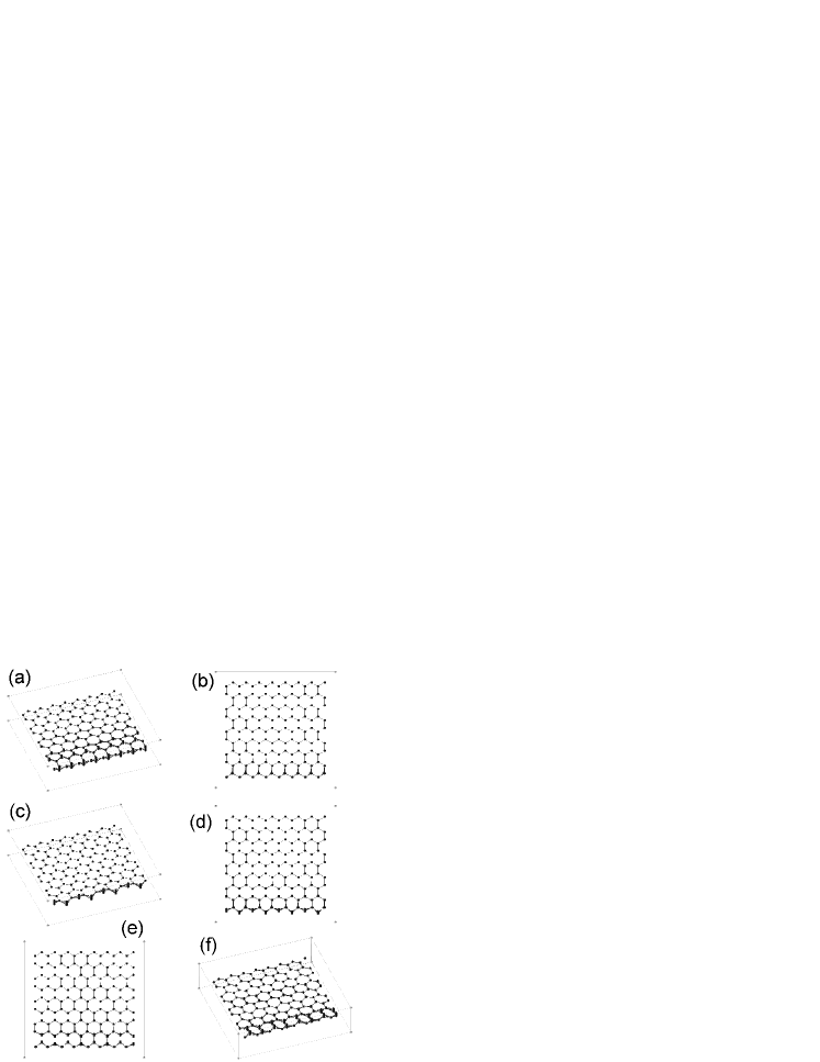
Figure 9: Six edge modes of the zigzag nanoribbon. Shown are the displacements of atoms of the nanoribbon at quarter of an oscillation period, for: (a) out-of-plane vibration with $\omega=583$ cm^-1, $q=0$; (b) in-plane vibration with $\omega=1466$ cm^-1, $q=0$; (c) out-of-plane vibration with $\omega=261$ cm^-1, $q=\pi$; (d) in-plane vibration with $\omega=393$ cm^-1, $q=\pi$; (e) in-plane vibration with $\omega=406$ cm^-1, $q=\pi$; (f) out-of-plane vibration with $\omega=431$ cm^-1, $q=\pi$. Mass of the edge atoms is $M_{1}=13m_{p}$.

V Longitudinal localization and surface solitons

The surface oscillations described above are localized at the edges of the stripe, and they correspond to quasi-one-dimensional excitations of the nanoribbon. Therefore, similar to other types of nonlinear modes, we may expect that such surface mode may experience the longitudinal localization with the formation of breather solitons. Such novel type of surface breathers exist due to the transverse energy localization in the surface state and nonlinearity-induced longitudinal localization along the nanoribbon edge.

To analyze the existence of breather solitons, we consider the nanoribbon of a fixed length and free edges with $N=500$ periods. We introduce friction at the far edges in order to absorb phonons propagating away from the localization region. To find spatially localized nonlinear states, we integrate numerically the system of equations (7) ($1\leq n\leq N$) with the initial conditions corresponding to a localized state at the edge of the nanoribbon,

$${\bf x}_{n}(t)=A_{n}{\bf e}\exp(iqn-i\omega t),$$ (11)

where $A_{n}=A\;{\rm sech}\{\mu[(n-N/2)+1/2]\}$, with the parameter $\mu>0$ characterizing the inverse width of the initial excitation, and the amplitude $A>0$. A complex unit $3M$-dimensional vector ${\bf e}={\bf e}_{r}+i{\bf e}_{i}$, a solution of the linear equation (10), corresponds to the edge mode with the wave numbers $q=0,~{}\pi$ and the frequency $\omega$.

For the system of equations (7), the ansatz (11) corresponds to the following initial conditions,

$${\bf x}_{n}(0) = A_{n}[{\bf e}_{r}\cos(q\tilde{n})-{\bf e}_{i}\sin(q\tilde{n})],$$ (12)

$$\dot{\bf x}_{n}(0) = A_{n}\omega[{\bf e}_{r}\sin(q\tilde{n})-{\bf e}_{i}\cos(q\tilde{n})],$$

where $\tilde{n}=n-N/2+1/2$.

The breather frequency can only split-off from one of the linear dispersion bands. As follows from Figs. 4 and 5, the frequency branches corresponding to the edge vibrations have either minimal or maximum values at $q=0$ and $q=\pi$, so that we use these values in the initial conditions (12).

By changing the value of the initial amplitude $A$ and the inverse width $\mu$, and analyzing the dynamics of the system (7) with the initial conditions (12), we may arrive at the conclusion if the system under consideration can support spatially localized states in the form of the breather solitons, as self-trapped nonlinear modes splitting-off from the corresponding edge of the linear dispersion band. If such a breather exists, the initial excitation (12) will experience no substantial spreading, whereas it will spread out if the breather conditions are not satisfied.

Our extensive numerical simulations reveal that the edge breather are not possible for the zigzag nanoribbons, and the initial excitation of the form (12) always spreads. However, for the armchair nanoribbons the longitudinal localization of the edge modes becomes possible with the wave number $q=\pi$ and frequency $\omega=102$ (out-of-plane vibration) and 268 cm^-1 (in-plane vibration), see Fig. 10. For the inverse width $\mu=0.05$ and amplitude $A=0.008$ Å, the initial localized vibrational state with the frequency $\omega=102$ cm^-1 decays slowly, but this decay stops when the initial amplitude is increased to the value $A=0.016$ Å, and it evolves into a localized breathing mode with the breather frequency 103 cm^-1. When we increase the initial amplitude to the value $A=0.032$ Å, we observe the generation of two breathers which interact nonlinearly.

Similarly, for the planar edge vibration with the frequency $\omega=268$ cm^-1 the initial localized state spreads when its amplitude is $A=0.004$ Å  [see Fig. 10(a)], it gets self-trapped for $A=0.008$ Å  and generates a breather with the frequency 267 cm^-1 [see Fig. 10(b)], and for $A=0.016$ Å  it creates two interacting breathers.

Our studies demonstrate that armchair nanoribbons can support two types of spatially localized surface breathers. One type of breathers originates from the localization of out-of-plane edge mode with the frequency $\omega=102$ cm^-1. This edge mode is shown in Fig. 8(c), where the edge atoms of the neighboring elementary cells oscillate with the opposite phases in the direction perpendicular to the nanoribbon plane. The other type of breathers originates from the longitudinal localization of the in-plane edge mode with the frequency $\omega=268$ cm^-1. This edge mode is shown in Fig. 8(f), where the edge atoms oscillate transversally in the nanoribbon plane. The frequency of the former breather grows with the amplitude, while the frequency of the latter breather decays with the amplitude, in accord with the structure of the dispersion curves presented in Fig. 4.

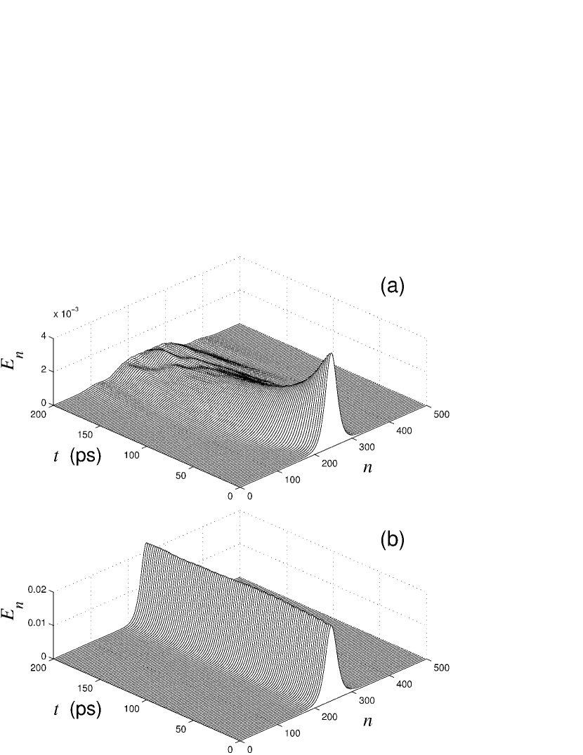
Figure 10: Dynamics of the initially localized edge excitation of the armchair nanoribbon (wave number $q=\pi$, frequency $\omega=268$ cm^-1, and inverse dimensionless width $\mu=0.05$) for the initial amplitude: (a) $A=0.004$ and (b) $A=0.008$ Å. Shown is the temporal evolution of the the kinetic energy $E_{n}$ in two first edge layers of atoms of the nanoribbon ($k=1$, 2, 3, 4). Mass of the edge atoms is $M_{1}=13m_{p}$.

VI Conclusions

We have demonstrated that both armchair and zigzag graphene nanoribbons can support various types of vibrational Tamm states in the form of phonons localized at the edges of the graphene stripe. We have shown that such localized modes appear in the gaps of the frequency spectrum of the nanoribbon oscillations, and they can be classified as in-plane and out-of-plane surface modes. In the former case, all atoms oscillate in the plane of the nanoribbon, whereas in the latter case the atoms oscillate perpendicular to the plane. We have found that some of these edge modes can experience self-localization along the nanoribbon edge with the formation of spatially localized breather solitons. Our molecular dynamics simulations have revealed the existence of two types of such breather solitons, out-of-plane vibrational breathers with the frequency 103 cm^-1 and in-plane breathers with the frequency 267 cm^-1.

References

- (1) K. S. Novoselov, A. K. Geim, S. V. Morozov, D. Jiang, Y. Zhang, S. V. Dubonos, I. V. Grigorieva, A. A. Firsov, G. W. C. Kaye, and T. H. Laby, Science 306, 666 (2004).
- (2) A. K. Geim and K. S. Novoselov, Nature Materials 6, 183 (2007).
- (3) M. I. Katsnelson, Materials Today 10, 20 (2007).
- (4) See, e.g., G. Lee and K. Cho, Phys. Rev. B 79, 165440 (2009), and references therein.
- (5) S. G. Davidson and M. Steslicka, Basic Theory of Surface States (Oxford Science Publications, New York, 1996).
- (6) I. Tamm, Phys. Z. Sowjetunion 1, 733 (1932).
- (7) W. Shockley, Phys. Rev. 56, 317 (1939).
- (8) A.A. Maradudin and G. Stegeman, in Surface Phonons, W. Kress and F.W. De Wette, eds. (Springer-Verlag, Berlin, 1991), pp. 5-35.
- (9) V. M. Agranovich and D. L. Mills, Surface Polaritons (North Holland, Amsterdam, 1984).
- (10) I. L. Garanovich, A. A. Sukhorukov, and Yu. S. Kivshar, Phys. Rev. Lett. 100, 203904 (2008).
- (11) A. Szameit, I. L. Garanovich, M. Heinrich, A. A. Sukhorukov, F. Dreisow, T. Pertsch, S. Nolte, A. Tunnermann, and Yu. S. Kivshar, Phys. Rev. Lett. 101, 203902 (2008).
- (12) M. Vandescuren, P. Hermet, V. Meunier, L. Henrard, and Ph. Lambin, Phys. Rev. B 78, 195401 (2008).
- (13) G. Lee and K. Cho, Phys. Rev. B 79, 165440 (2009).
- (14) D. W. Boukhvalov and M. I. Katsnelson, Nano Letters 8, 4373 (2008).
- (15) D. W. Noid, B. G. Sumpter, and B. Wunderlich, Macromolecules 24, 4148 (1991).
- (16) B. G. Sumpter, D. W. Noid, G. L. Liang, and B. Wunderlich, Adv. Polym. Sci. 116, 27 (1994).
- (17) A.V. Savin and L.I. Manevitch, Phys. Rev. B 58, 11386 (1998).
- (18) A.V. Savin and L.I. Manevitch, Phys. Rev. E 61, 7065 (2000).
- (19) A. V. Savin and L. I. Manevitch, Phys. Rev. B 67, 144302 (2003).
- (20) A. V. Savin and Yu. S. Kivshar, Europhys. Letters 82, 66002 (2008).
- (21) D. Gunlycke, H. M. Lawler, and C. T. White, Phys. Rev. B 77, 014303 (2008).
- (22) R. Al-Jishi and G. Dresselhaus, Phys. Rev. B 26, 4514 (1982).
- (23) T. Aizawa, R. Souda, S. Otani, Y. Ishizawa, and C. Oshima, Phys. Rev. B 42, 11469 (1990).