Chaotic vibrations and strong scars

1. Introduction

What relates an earthquake, a drum, a 2-dimensional mesoscopic cavity, a microwave oven and an optical fibre? The equations governing wave propagation in these systems (seismic, acoustic, electronic, microwave and optical) are linear. As a result, the solutions of the wave equations can be decomposed as a sum over vibrating eigenmodes (or stationary modes). The discrete (or “quantum”) nature of this eigenmode decomposition is due to the compact geometry of the above-mentioned “cavities”. Mathematically, the latter are modelled by compact, $d$-dimensional Riemannian manifolds $(X,g)$ with or without boundaries.

To simplify the presentation, we will restrict ourselves to scalar waves, described by a real wavefunction $\psi(x,t)$. The eigenmodes $(\psi_{n}(x))_{n\geq 0}$ then satisfy Helmholtz’s equation

(1.1) $$\Delta\psi_{n}+k_{n}^{2}\,\psi_{n}=0\,,$$

where $\Delta:H^{2}\to L^{2}$ is the Laplace-Beltrami operator on $X$ and $k_{n}\geq 0$ is the vibration frequency of the mode $\psi_{n}$. If the manifold has a boundary (as is the case for an acoustic drum or for electromagnetic cavities), the wavefunction must generally satisfy specific boundary conditions, dictated by the physics of the system: the simplest ones are the Dirichlet ($\psi_{|\partial X}=0$) and Neumann ($\partial_{\nu}\psi_{|\partial X}=0$) boundary conditions, where $\partial_{\nu}$ is the normal derivative at the boundary.

Our goal is to describe the eigenmodes, in particular the high-frequency eigenmodes ($k_{n}\gg 1$). Specifically, we would like to predict the localization properties of the modes $\psi_{n}$, from our knowledge of the geometry of the manifold $(X,g)$.

Consider, for instance, the case of a bounded domain in the Euclidean plane, which we will call a billiard. For some very particular billiard shapes (e.g. a rectangle, a circle or an ellipse), there exists a choice of coordinates allowing one to separate the variables in Helmholtz’s equation (1.1), thereby reducing it to a one-dimensional eigenvalue problem (of the Sturm-Liouville type). In the high-frequency limit, the latter can be solved to arbitrarily high precision through WKB methods, or sometimes even exactly (see Figure 1.1). The high-energy eigenmodes of such domains are hence very well-understood.

This separation of variables can be interpreted as a particular symmetry of the classical dynamics of the billiard (the motion of a point particle rolling frictionless across the billiard and bouncing on its boundary). This dynamics is Liouville-integrable, which means that there is a conserved quantity in addition to the kinetic energy. For instance, in a circular billiard the angular momentum of the particle is conserved. The classical trajectories are then very “regular” (see Figure 1.1). The same regularity is observed in the eigenfunctions and can be explained by the existence of a non-trivial differential operator commuting with the Laplacian.

  

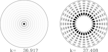
Figure 1.1. Left: one orbit of the circular billiard. Center and right: two eigenmodes of that billiard, with their respective frequencies.

As soon as an integrable billiard is slightly deformed, the symmetry is broken: the geodesic flow is no longer integrable; it becomes chaotic in some regions of phase space. We do not have any approximate formula at hand to describe the eigenmodes. The extreme situation consists of fully chaotic billiards, like the “stadium” displayed in Figure 1.2 (the word “chaotic” is a fuzzy notion; the results we present below will always rely on precise mathematical assumptions).

We mention that the most recent numerical methods (the boundary operator and the “scaling method”) allow one to compute a few tens of thousands of eigenmodes for 2-dimensional billiards, at most a few thousands in 3 dimensions and much less if the metric is not Euclidean. The difficulty stems from the fact that a mode of frequency $k_{n}\gg 1$ oscillates on a scale $\sim 1/k_{n}$ (the wavelength); one thus needs a finer and finer mesh when increasing the frequency. On the other hand, the analytical methods and results we present below are especially fitted to describe these high-frequency modes.

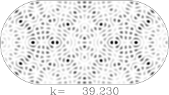
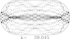
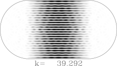
Figure 1.2. Top left: one typical “ergodic” orbit of the “stadium”: it equidistribues across the whole billiard. The three other plots feature eigenmodes of frequencies $k_{n}\approx 39$. Bottom left: a “scar” on the (unstable) horizontal periodic orbit. Bottom right: a “bouncing ball” mode.

1.1. Semiclassical methods

In the general case of a Riemannian manifold, the classical dynamics (away from the boundaries) consists of the Hamiltonian flow $g^{t}$ on the cotangent bundle $T^{*}X$, generated by the free motion Hamiltonian

(1.2) $$H(x,\xi)=\frac{|\xi|^{2}}{2},\quad(x,\xi)\in T^{*}X.$$

The flow on the energy layer $H^{-1}(1/2)=S^{*}X=\{(x,\xi)\,:\,|\xi|=1\}$ is simply the geodesic flow on the manifold (with reflections on the boundary in the case $\partial X\neq 0$).

The high-frequency regime allows us to use the tools of semiclassical analysis. Indeed, the Helmholtz equation (1.1) can be interpreted as a stationary Schrödinger equation: taking $\hbar_{n}=k_{n}^{-1}$ as an “effective Planck’s constant”, the eigenmode $\psi_{n}$ satisfies

(1.3) $$-\frac{\hbar_{n}^{2}\Delta}{2}\,\psi_{n}=\frac{1}{2}\,\psi_{n}.$$

The operator $-\frac{\hbar^{2}\Delta}{2}$ on the left-hand side is the quantum Hamiltonian governing the dynamics of a particle moving freely inside the cavity; it is the quantization of the classical Hamiltonian (1.2). The above equation describes a quantum particle in a stationary state of energy $E=1/2$ (in this formalism, the energy is fixed but Planck’s “constant” is the running variable). The high-frequency limit $k_{n}\to\infty$ exactly corresponds to the semiclassical regime $\hbar=\hbar_{n}\to 0$. In the following, the eigenmode will be denoted by $\psi_{n}$ or $\psi_{\hbar}$.

The correspondence principle provides a connection between the Schrödinger propagator, namely the unitary flow $U^{t}=e^{{it\hbar}\frac{\Delta}{2}}$ acting on $L^{2}(X)$ and the geodesic flow $g^{t}$ acting on the phase space $T^{*}X$. The former “converges” towards the latter in the semiclassical limit $\hbar\to 0$, in a sense made explicit below. The aim of semiclassical analysis is to exploit this correspondence and use our understanding of the geodesic flow in order to extract properties of the Schrödinger flow.

To analyse the eigenmodes we need to observe them by using quantum observables. For us, an observable is a real function $A\in C^{\infty}(T^{*}X)$ that will be used as a test function to measure the phase space localization of a wavefunction. One can associate to this function a quantum observable $\operatorname{Op}_{\hbar}(A)$, which is a selfadjoint operator on $L^{2}(X)$ obtained from $A$ through a certain ($\hbar$-dependent) quantization procedure. For instance, on $X=\mathbb{R}^{d}$ a possible procedure is the Weyl quantization

(1.4) $$\operatorname{Op}_{\hbar}^{W}(A)f(x)=\frac{1}{(2\pi\hbar)^{d}}\int A\left(\frac{x+y}{2},\xi\right)e^{\frac{i}{\hbar}\xi.(x-y)}f(y)dy\,d\xi.$$

The simplest case consists of functions $A(x,\xi)=A(x)$ independent of the momentum; $\operatorname{Op}_{\hbar}^{W}(A)$ is then the operator of multiplication by $A(x)$. If $A=A(\xi)$ is a polynomial in the variable $\xi$ then $\operatorname{Op}_{\hbar}^{W}(A)$ is the differential operator $A\left(\frac{\hbar}{i}\frac{\partial}{\partial x}\right)$. The role of the parameter $\hbar$ in the definition of $\operatorname{Op}_{\hbar}^{W}(A)$ is to adapt that operator to the study of functions oscillating on a spatial scale $\sim\hbar$. On a general smooth manifold $X$, one can define a quantization $\operatorname{Op}_{\hbar}(A)$ by using the formula (1.4) in local charts and then glue together the charts using a smooth partition of unity.

A mathematical version of the correspondence principle takes the form of an Egorov theorem. It states that quantization (approximately) commutes with evolution for observables:

(1.5) $$\|e^{-it\hbar\frac{\Delta}{2}}\operatorname{Op}_{\hbar}(A)e^{{it\hbar}\frac{\Delta}{2}}-\operatorname{Op}_{\hbar}(A\circ g^{t})\|_{\mathcal{L}(L^{2})}=\mathcal{O}_{A,t}(\hbar)\,.\quad\text{{(Egorov)}}$$

1.2. Semiclassical measures

In quantum mechanics, the function $|\psi(x)|^{2}$ describes the probability (density) of finding the particle at the position $x\in X$. A measuring device will only be able to measure the probability integrated over a small region (a “pixel”) $\int_{B}|\psi(x)|^{2}\,dx$, which can be expressed as a diagonal matrix element $\langle\psi,{\mathchoice{1\mskip-4.0mu{\rm{l}}}{1\mskip-4.0mu{\rm{l}}}{1\mskip-4.5mu{\rm{l}}}{1\mskip-5.0mu{\rm{l}}}}_{B}\psi\rangle$. Here ${\mathchoice{1\mskip-4.0mu{\rm{l}}}{1\mskip-4.0mu{\rm{l}}}{1\mskip-4.5mu{\rm{l}}}{1\mskip-5.0mu{\rm{l}}}}_{B}$ is the multiplication operator (on $L^{2}(X)$) by the characteristic function on $B$.

More generally, for a nontrivial observable $A(x,\xi)$ supported in a small phase space region, the matrix element $\langle\psi,\operatorname{Op}_{\hbar}(A)\psi\rangle$ provides information on the probability of the particle lying in this region. From the linearity of the quantization scheme $A\mapsto\operatorname{Op}_{\hbar}(A)$, this matrix element defines a distribution $\mu_{\psi}$ on $T^{*}X$:

$$\mu_{\psi}(A)\stackrel{{\scriptstyle\rm{def}}}{{=}}\langle\psi,\operatorname{Op}_{\hbar}(A)\psi\rangle,\qquad\forall A\in C_{0}^{\infty}(T^{*}X).$$

This distribution (which depends on the state $\psi$ but also on the scale $\hbar$) is called the Wigner measure of the state $\psi$. The projection of $\mu_{\psi}$ on $X$ is equal to the probability measure $|\psi(x)|^{2}\,dx$; for this reason, $\mu_{\psi}$ is also called a microlocal lift of that measure. Still, $\mu_{\psi}$ contains more information: it takes the phase of $\psi$ into account and thereby also describes the local momentum of the particle (measured at the scale $\hbar$).

In order to study the localization properties of the eigenmodes $\psi_{n}$, we will consider their Wigner measures $\mu_{\psi_{n}}=\mu_{n}$ (constructed with the adapted scales $\hbar_{n}$). It is difficult to state anything rigorous about the Wigner measures of individual eigenmodes so we will only aim to understand the limits of (subsequences of) the family $(\mu_{n})_{n\geq 0}$ in the weak topology on distributions. Such a limit $\mu$ is called a semiclassical measure of the manifold $X$. Basic properties of the quantization scheme imply that:

• $\mu$ is a probability measure supported on the energy shell $S^{*}X$.

• $\mu$ is invariant through the geodesic flow: $\mu=(g^{t})_{*}(\mu)$, $\forall t\in\mathbb{R}$.

• The collection of semiclassical measures $\mu$ does not depend on the choices of local symplectic coordinates involved in the definition of the quantization scheme $A\mapsto\operatorname{Op}_{\hbar}(A)$.

The second property is a direct consequence of the Egorov theorem (1.5).

Starting from the family of quantum stationary modes $(\psi_{n})_{n}$, we have constructed one or several probability measures $\mu$ on $S^{*}X$, invariant through the classical flow. Each of them describes the asymptotical localization properties of the modes in some subsequence $(\psi_{n_{j}})_{j\geq 1}$.

1.3. Is any invariant measure a semiclassical measure?

On a general Riemannian manifold $X$, the geodesic flow admits many different invariant probability measures. The Liouville measure, defined as the disintegration on the energy shell $S^{*}X$ of the symplectic volume $dx\,d\xi$, is a “natural” invariant measure on $S^{*}X$. We will denote it by $L$ in the following. Furthermore, each periodic geodesic carries a unique invariant probability measure. The chaotic flows we will consider admit a countable set of periodic geodesics, the union of which fills $S^{*}X$ densely.

Given a manifold $(X,g)$, we are led to the following question: Among all $g^{t}$-invariant probability measures on $S^{*}X$, which ones do actually appear as semiclassical measures? Equivalently, to which invariant measures can the Wigner measures $(\mu_{n})$ converge to in the high-frequency limit?

At the moment, the answer to this question for a general manifold $X$ is unknown. We will henceforth be less ambitious and restrict ourselves to geodesic flows satisfying well-controlled dynamical properties: the strongly chaotic systems.

2. Chaotic geodesic flows

The word “chaotic” is quite vague so we will need to provide more precise dynamical assumptions. All chaotic flows we will consider are ergodic with respect to the Liouville measure. This means that $S^{*}X$ cannot be split into two invariant subsets of positive measures. A more “physical” definition is the following: the trajectory starting on a typical point $\rho\in S^{*}X$ will cover $S^{*}X$ in a uniform way at long times (see Figure 1.2) so that “time average equals spatial average”.

The “stadium” billiard (see Figure 1.2) enjoys a stronger chaoticity: mixing, meaning that any (small) ball $B\subset S^{*}X$ evolved through the flow will spread uniformly throughout $S^{*}X$ for large times. The strongest form of chaos is reached by the geodesic flow on a manifold of negative curvature; such a flow is uniformly hyperbolic or, equivalently, it has the Anosov property [3]. All trajectories are then unstable with respect to small variations of the initial conditions. Paradoxically, this strong instability leads to a good mathematical control on the long time properties of the flow. Such a flow is fast mixing with respect to $L$.

Numerical computations of eigenmodes are easier to perform for Euclidean billiards than on curved manifolds; on the other hand, the semiclassical analysis is more efficient in the case of boundary-free compact manifolds so most rigorous results below concern the latter.

2.1. Quantum ergodicity

Ergodicity alone already strongly constrains the structure of the high-frequency eigenmodes: almost all of these eigenmodes are equidistributed on $S^{*}X$.

Theorem 2.1 (Quantum ergodicity).

[22, 24, 9] Assume the geodesic flow on $(X,g)$ is ergodic with respect to the Liouville measure on $S^{*}X$.

Then, there exists a subsequence $(n_{j})\subset\mathbb{N}$ of density $1$ such that the Wigner measures of the corresponding eigenmodes satisfy

$$\mu_{n_{j}}\mathop{\longrightarrow}\limits_{j\to\infty}L\,.$$

The phrase “of density $1$” means that $\frac{\#\{n_{j}\leq N\}}{N}\stackrel{{\scriptstyle N\to\infty}}{{\to}}1$. Therefore, if there exists a subsequence of eigenmodes converging towards a semiclassical measure $\mu\neq L$, this subsequence must be sparse and consist of exceptional eigenmodes.

2.2. “Scars” and exceptional semiclassical measures

Numerical computations of eigenmodes of some chaotic billiards have revealed interesting structures. In 1984, Heller [15] observed that some eigenmodes of the “stadium” billiard (the ergodicity of which had been demonstrated by Bunimovich) are “enhanced” along some periodic geodesics. He called such an enhancement a “scar” of the periodic geodesic upon the eigenmode (see Figure 1.2). Although it is well-understood that an eigenmode can be concentrated along a stable periodic geodesic, the observed localization along unstable geodesics is more difficult to justify. The enhancement observed by Heller was mostly “visual”; the more quantitative studies that followed Heller’s paper (e.g. [5]) seem to exclude the possibility of a positive probability weight remaining in arbitrary small neighbourhoods of the corresponding geodesic. Such a positive weight would have indicated that the corresponding semiclassical measures “charge” the unstable orbit (a phenomenon referred to as “strong scar” in [21]). Contrary to the case of Euclidean billiards, numerical studies on surfaces of constant negative curvature have not shown the presence of “scars” [4].

On the mathematical level, the most precise results on the localization of eigenmodes are obtained in the case of certain surfaces of constant negative curvature enjoying specific arithmetic symmetries, called “congruence surfaces”. A famous example is the modular surface (which is not compact). For these surfaces, there exists a commutative algebra of selfadjoint operators on $L^{2}(X)$ (called Hecke operators), which also commute with the Laplacian. It is then reasonable to focus on the orthonormal bases formed of joint eigenmodes of these operators (called Hecke eigenmodes). Rudnick and Sarnak have shown [21] that semiclassical measures associated with such bases cannot charge any periodic geodesic (“no strong scar” on congruence surfaces). This result, as well as the numerical studies mentioned above, suggested to them the following

Conjecture 2.2 (Quantum unique ergodicity).

Let $(X,g)$ be a compact Riemannian manifold of negative curvature. For any orthonormal eigenbasis of the Laplacian, the sequence of Wigner measures $(\mu_{n})_{n\geq 0}$ admits a unique limit (in the weak topology), namely the Liouville measure.

This conjecture goes far beyond the non-existence of “strong scars”. It also excludes all the “fractal” invariant measures.

This conjecture has been proved by E. Lindenstrauss in the case of compact congruence surfaces, provided one only considers Hecke eigenbases [18]. The first part of the proof [7] (which relies heavily on the Hecke algebra) consists of estimating from below the entropies of the ergodic components of a semiclassical measure. We will see below that the entropy is also at the heart of our results.

2.3. The role of multiplicity?

A priori, there can be multiple eigenvalues in the spectrum of the Laplacian, in which case one can make various choices of orthonormal eigenbases. On a negatively curved surface, it is known [6] that the eigenvalue $k_{n}^{2}$ has multiplicity $\mathcal{O}\left(\frac{k_{n}}{\log k_{n}}\right)$ but this is far from what people expect, namely a uniformly bounded multiplicity. One could modify Conjecture 2.2 so that the statement holds for a given basis (e.g. a Hecke eigenbasis in the case of a congruence surface) but may be false for another basis.

In parallel with the study of chaotic geodesic flows, people have also considered toy models of discrete time symplectic transformations on some compact phase spaces. The most famous example of such transformations is better known as “Arnold’s cat map” on the 2-dimensional torus. It consists of a linear transformation $(x,\xi)\to M(x,\xi)$, where the unimodular matrix $M\in SL(2,\mathbb{Z})$ is hyperbolic, i.e. it satisfies $|{\rm tr}M|>2$. The “Anosov property” then results from the fact that no eigenvalue of $M$ has modulus $1$. That transformation can be quantized to produce a family of unitary propagators, depending on a mock Planck parameter $\hbar_{N}=(2\pi N)^{-1}$, where $N$ is an integer [14]. Such propagators have been named “quantum maps” and have served as a “laboratory” for the study of quantum chaotic systems, both on the numerical and analytical sides.

Concerning the classification of semiclassical measures, the “quantized cat map” has exhibited unexpectedly rich features. On the one hand, this system enjoys arithmetic symmetries, allowing one to define “Hecke eigenbases” and prove the quantum unique ergodicity for such eigenbases [16]. On the other hand, for some (scarce) values of $N$ the spectrum of the quantum propagator contains large degeneracies. This fact has been exploited in [10] to construct sequences of eigenfunctions violating quantum unique ergodicity: the corresponding Wigner measures $\mu_{N}$ converge to the semiclassical measure

(2.1) $$\mu=\frac{1}{2}\delta_{O}+\frac{1}{2}L,$$

where $L=dx\,d\xi$ is now the symplectic volume measure and $\delta_{0}$ is the $M$-invariant probability measure supported on a periodic orbit of $M$.

This result shows that the quantum unique ergodicity conjecture can be wrong when extended to chaotic systems more general than geodesic flows. More precisely, for the “cat map” the conjecture holds true for a certain eigenbasis but is wrong for another one.

Another result concerning the “cat map” is the following: the weight $1/2$ carried by the scar in (2.1) is maximal [11]. In particular, no semiclassical measure can be supported on a countable union of periodic orbits. In the next section, dealing with our more recent results on Anosov geodesic flows, we will see this factor $1/2$ reappear.

3. Entropic bounds on semiclassical measures

In this section, we consider the case of a compact manifold (without boundary) of negative sectional curvature. As mentioned earlier, the corresponding geodesic flow has many invariant probability measures. The Kolmogorov-Sinai entropy associated with an invariant measure is a number $h_{KS}(\mu)\geq 0$, defined below. We stress a few important properties:

• A measure supported by a periodic trajectory has zero entropy.

• The maximal entropy $h_{\max}$ is reached for a unique invariant measure, called the Bowen-Margulis measure, of support $S^{*}X$.

• According to the Ruelle-Pesin inequality,

  (3.1) $$h_{KS}(\mu)\leq\int\sum_{k=1}^{d-1}\lambda_{k}^{+}d\mu,$$

  where the functions $\lambda_{1}^{+}(\rho)\geq\lambda^{+}_{2}(\rho)\geq\cdots\geq\lambda_{d-1}(\rho)>0$, defined $\mu$-almost everywhere, are the positive Lyapunov exponents of the flow. Equality in (3.1) is reached only if $\mu$ is the Liouville measure [17].

• On a manifold of constant curvature $-1$, the inequality reads $h_{KS}(\mu)\leq d-1$. The Bowen-Margulis measure is then equal to the Liouville measure.

• The functional $h_{KS}$ is affine on the convex set of invariant probability measures.

These properties show that the entropy provides a quantitative indication of the localization of an invariant measure. For instance, a positive lower bound on the entropy of a measure implies that it cannot be supported by a countable union of periodic geodesics. This is precisely the content of our first result.

Theorem 3.1.

(1) [1] Let $X$ be a compact Riemannian manifold such that the geodesic flow has the Anosov property. Then every semiclassical measure $\mu$ on $S^{*}X$ satisfies

$$h_{KS}(\mu)>0.$$

(2) [2] Under the same assumptions, let $\lambda_{j}^{+}(\rho)$ be the positive Lyapunov exponents and $\lambda_{\max}=\lim_{t\to\infty}\frac{1}{t}\log\sup_{\rho\in S^{*}X}||dg^{t}_{\rho}||$ be the maximal expansion rate of the geodesic flow. Then the entropy of $\mu$ satisfies

(3.2) $$h_{KS}(\mu)\geq\int\sum_{k=1}^{d-1}\lambda_{k}^{+}d\mu-\frac{d-1}{2}\lambda_{\max}\,.$$

In constant curvature $-1$, this bound reads $h_{KS}(\mu)\geq\frac{d-1}{2}$.

Corollary 1.

[1] Let $X$ be a compact manifold of dimension $d$ and constant sectional curvature $-1$. Then, for any semiclassical measure $\mu$, the support of $\mu$ has Hausdorff dimension $\geq d$.

In constant negative curvature, the lower bound $h_{KS}(\mu)\geq\frac{d-1}{2}$ implies that at most $1/2$ of the mass of $\mu$ can consist of a scar on a periodic orbit. This is in perfect agreement with the similar result proved for “Arnold’s cat map” (see §2.3).

The right-hand side of (3.2) can be negative if the curvature varies a lot, which unfortunately makes the result trivial. A more natural lower bound to hope for would be

(3.3) $$h_{KS}(\mu)\geq\frac{1}{2}\int\sum_{k=1}^{d-1}\lambda_{k}^{+}d\mu.$$

This lower bound has been obtained recently by G. Rivière for surfaces ($d=2$) of nonpositive curvature [20]. B. Gutkin has proved an analogous result for certain quantum maps with a variable Lyapunov exponent [12]; he also constructed eigenstates for which the lower bound is attained.

From the Ruelle–Pesin inequality (3.1), we notice that proving the quantum unique ergodicity conjecture in the case of Anosov geodesic flows would amount to getting rid of the factor $1/2$ in (3.3).

We finally provide a definition of the entropy and a short comparison between the entropy bound of Bourgain-Lindenstrauss [7] and ours.

Definition 1.

The shortest definition of the entropy results from a theorem due to Brin and Katok [8]. For any time $T>0$, introduce a distance on $S^{*}X$,

$$d_{T}(\rho,\rho^{\prime})=\max_{t\in[-T/2,T/2]}d(g^{t}\rho,g^{t}\rho^{\prime}),$$

where $d$ is the distance built from the Riemannian metric. For $\epsilon>0$, denote by $B_{T}(\rho,\epsilon)$ the ball of centre $\rho$ and radius $\epsilon$ for the distance $d_{T}$. When $\epsilon$ is fixed and $T$ goes to infinity, it looks like a thinner and thinner tubular neighbourhood of the geodesic segment $[g^{-\epsilon}\rho,g^{+\epsilon}\rho]$ (this tubular neighbourhood is of radius $e^{-T/2}$ if the curvature of $X$ is constant and equal to $-1$).

Let $\mu$ be a $g^{t}$–invariant probability measure on $S^{*}X$. Then, for $\mu$-almost every $\rho$, the limit

$$\lim_{\epsilon\longrightarrow 0}\,\liminf_{T\longrightarrow+\infty}-\frac{1}{T}\log\mu\big{(}B_{T}(\rho,\epsilon)\big{)}\\ =\lim_{\epsilon\longrightarrow 0}\,\limsup_{T\longrightarrow+\infty}-\frac{1}{T}\log\mu\big{(}B_{T}(\rho,\epsilon)\big{)}\stackrel{{\scriptstyle\rm{def}}}{{=}}h_{KS}(\mu,\rho)$$

exists and it is called the local entropy of the measure $\mu$ at the point $\rho$ (it is independent of $\rho$ if $\mu$ is ergodic). The Kolmogorov-Sinai entropy is the average of the local entropies:

$$h_{KS}(\mu)=\int h_{KS}(\mu,\rho)d\mu(\rho).$$

Remark 3.2.

In the case of congruence surfaces, Bourgain and Lindenstrauss [7] proved the following bound on the microlocal lifts of Hecke eigenbases: for any $\rho$, and all $\epsilon>0$ small enough,

$$\mu_{n}\big{(}B_{T}(\rho,\epsilon)\big{)}\leq Ce^{-T/9},$$

where the constant $C$ does not depend on $\rho$ or $n$. This immediately yields that any semiclassical measure associated with these eigenmodes satisfies $\mu(B_{T}(\rho,\epsilon))\leq Ce^{-T/9}$, which implies that any ergodic component of $\mu$ has entropy $\geq\frac{1}{9}$.

In [2], we work with a different, but equivalent, definition of the entropy. On a manifold of dimension $d$ and constant curvature $-1$, the bound we prove can be (at least intuitively) interpreted as

(3.4) $$\mu_{n}\big{(}B_{T}(\rho,\epsilon)\big{)}\leq C\,k_{n}^{\frac{d-1}{2}}\,e^{-\frac{(d-1)T}{2}},$$

where $k_{n}^{2}$ is the eigenvalue of the Laplacian associated with $\psi_{n}$. This bound only becomes non-trivial for times $T>\log k_{n}$. For this reason, we cannot directly deduce bounds on the weights $\mu(B_{T}(\rho,\epsilon))$; the link between (3.4) and the entropic bounds of Theorem 3.1 is less direct and uses some specific features of quantum mechanics.

References

- [1] N. Anantharaman, Entropy and the localization of eigenfunctions, Ann. of Math. 168 435–475 (2008)
- [2] N. Anantharaman, S. Nonnenmacher, Half-delocalization of eigenfunctions of the Laplacian on an Anosov manifold, Ann. Inst. Fourier 57, 2465–2523 (2007); N. Anantharaman, H. Koch and S. Nonnenmacher, Entropy of eigenfunctions, communication at International Congress of Mathematical Physics, Rio de Janeiro, 2006; arXiv:0704.1564
- [3] D. V. Anosov, Geodesic flows on closed Riemannian manifolds of negative curvature, Trudy Mat. Inst. Steklov. 90, (1967)
- [4] R. Aurich and F. Steiner, Statistical properties of highly excited quantum eigenstates of a strongly chaotic system, Physica D 64, 185–214 (1993)
- [5] A. H. Barnett, Asymptotic rate of quantum ergodicity in chaotic Euclidean billiards, Comm. Pure Appl. Math. 59, 1457–1488 (2006)
- [6] P. Bérard, On the wave equation on a compact Riemannian manifold without conjugate points, Math. Z. 155 (1977), no. 3, 249–276.
- [7] J. Bourgain, E. Lindenstrauss, Entropy of quantum limits, Comm. Math. Phys. 233, 153–171 (2003)
- [8] M. Brin, A. Katok, On local entropy, Geometric dynamics (Rio de Janeiro, 1981), 30–38, Lecture Notes in Math., 1007, Springer, Berlin, 1983.
- [9] Y. Colin de Verdière, Ergodicité et fonctions propres du Laplacien, Commun. Math. Phys. 102, 497–502 (1985)
- [10] F. Faure, S. Nonnenmacher and S. De Bièvre, Scarred eigenstates for quantum cat maps of minimal periods, Commun. Math. Phys. 239, 449–492 (2003).
- [11] F. Faure and S. Nonnenmacher, On the maximal scarring for quantum cat map eigenstates, Commun. Math. Phys. 245, 201–214 (2004)
- [12] B. Gutkin, Entropic bounds on semiclassical measures for quantized one-dimensional maps, arXiv:0802.3400
- [13] A. Hassell, Ergodic billiards that are not quantum uniquely ergodic, with an appendix by A. Hassell and L. Hillairet, arXiv:0807.0666
- [14] J. H. Hannay and M. V. Berry, Quantisation of linear maps on the torus – Fresnel diffraction by a periodic grating, Physica D 1, 267–290 (1980)
- [15] E. J. Heller, Bound-state eigenfunctions of classically chaotic Hamiltonian systems: scars of periodic orbits, Phys. Rev. Lett. 53, 1515–1518 (1984)
- [16] P. Kurlberg and Z. Rudnick, Hecke theory and equidistribution for the quantization of linear maps of the torus, Duke Math. J. 103, 47–77 (2000)
- [17] F. Ledrappier, L.-S. Young, The metric entropy of diffeomorphisms. I. Characterization of measures satisfying Pesin’s entropy formula, Ann. of Math. 122, 509–539 (1985)
- [18] E. Lindenstrauss, Invariant measures and arithmetic quantum unique ergodicity, Ann. of Math. 163, 165-219 (2006)
- [19] H. Maassen and J. B. M. Uffink, Generalized entropic uncertainty relations, Phys. Rev. Lett. 60, 1103–1106 (1988)
- [20] G. Rivière, Entropy of semiclassical measures in dimension 2, arXiv:0809.0230
- [21] Z. Rudnick and P. Sarnak, The behaviour of eigenstates of arithmetic hyperbolic manifolds, Commun. Math. Phys. 161, 195–213 (1994)
- [22] A. Shnirelman, Ergodic properties of eigenfunctions, Usp. Math. Nauk. 29, 181–182 (1974)
- [23] E. Vergini and M. Saraceno, Calculation by scaling of highly excited states of billiards, Phys. Rev. E 52, 2204 (1995)
- [24] S. Zelditch, Uniform distribution of the eigenfunctions on compact hyperbolic surfaces, Duke Math. J. 55, 919–941 (1987)