Broadband noise decoherence in solid-state complex architectures

Abstract

Broadband noise represents a severe limitation towards the implementation of a solid-state quantum information processor. Considering common spectral forms, we propose a classification of noise sources based on the effects produced instead of on their microscopic origin. We illustrate a multi-stage approach to broadband noise which systematically includes only the relevant information on the environment, out of the huge parametrization needed for a microscopic description. We apply this technique to a solid-state two-qubit gate in a fixed coupling implementation scheme.

1 Introduction

Building scalable multi-qubit systems is presently the main challenge towards the implementation of a solid-state quantum information processor [1]. High-fidelity single qubit gates based both on semi- [2] and super-conducting technologies are nowadays available. In particular, for the three basic types of superconducting qubits (charge, flux and phase) single-qubit operations with high quality factor have been demonstrated in different laboratories [3, 4]. Further improvement has been recently achieved with circuit-QED architectures [5, 6]. Multi-qubit systems instead have been proved harder to operate, the main limitation arising from the broadband solid state noise. The requirements for building an elementary quantum processor are in fact quite demanding on the efficiency of the protocols. This includes both severe constraints on readout and a sufficient isolation from fluctuations to reduce decoherence effects.

Based on experiments on the different Josephson junction (JJ) setups, there is presently a general consensus on the most common noise spectral forms and on the main consequences on systems evolutions. Typically noise is broadband and structured, i. e. the noise spectrum extends to several decades, it is non-monotonic, sometimes a few resonances are present.

Noise with $1/f$ spectrum is common to virtually all nanodevices. Its physical origin varies from device to device and depends on the specific material. Different implementations are in fact more sensitive either to charge, flux or to critical current fluctuations with spectral density scaling as the inverse of the frequency. The presence of slow components in the environment makes the decay of the coherent signal strongly dependent on the experimental protocol being used [4, 7, 8, 9]. Measurements protocols requiring numerous repetitions are particularly sensitive to the unstable device calibration due to low-frequency fluctuations. The leading effect is defocusing of the measured signal, analogous to inhomogeneous broadening in NMR [10]. The intrinsic high-frequency cut-off of $1/f$ noise is hardly detectable, measurements typically extending to $100$ Hz (recently charge noise up to $10$ MHz has been detected in a SET [11]). Incoherent energy exchanges between system and environment, leading to relaxation and decoherence, occur at typical operating frequencies (about $10$ GHz). Indirect measurements of noise spectrum in this frequency range often suggest a white or ohmic behavior [12, 13]. In addition, narrow resonances at selected frequencies (sometimes resonant with the nanodevice relevant energy scales) have being observed [14, 15]. In certain devices they originate from the circuitry [16] and may eventually be reduced by circuit design. More often, resonances are signatures of the presence of spurious fluctuators which also show up in the time resolved evolution, unambiguously proving the discrete nature of the noise sources [17]. Such fluctuators may severely limit the reliability of nanodevices [9, 18].

Explanation of this rich physics is beyond phenomenological theories describing the environment as a set of harmonic oscillators. On the other side, an accurate characterization of the noise sources might be a priory inefficient, since a huge number of parameters would be required for a microscopic description. Therefore one may follow a different route, consisting in classifying noise sources on the basis of their effects instead of on their nature and to understand, case by case, which is the efficient description of the environment. The required information may in fact depend on the specific protocol, especially when the environment is long-time correlated. This program is meaningful for quantum information where relevant time scales are much smaller than the decoherence time. This means that in the generic favorable situation coupling with the environment has simple effects on the system dynamics. As a difference with condensed matter physics where long time behavior is emphasized and interesting problems involve entanglement of a many-body system.

Here we illustrate a road-map to treat broadband noise which allows to obtain reasonable approximations by systematically including only the relevant information on the environment, out of the huge parametrization needed to specify it. The multi-stage approach for the different classes of broadband noise has been originally introduced for single qubit gates [9]. The obtained predictions for the decay of the coherent signal are in agreement with observations in various JJ implementations and in different protocols [8, 9]. We mention the observed decay of Ramsey fringes in charge-phase qubits [4] and recent results on flux/phase qubits [19]. Here we extend the procedure to complex solid-state architectures. As an illustrative case, we perform a systematic analysis of the effects and interplay of low and high frequency noise components in a two-qubit gate in a fixed coupling scheme. Such a systematic analysis points out that efficient operations in the solid state require an accurate preliminary characterization of the noise spectral characteristics and tuning appropriately the device working point.

The paper is organized as follows: in Section 2 we introduce the general framework of solid-state multi qubit gates and illustrate the characteristics of the most common spectral forms. In Section 3 we propose a classification of the noise sources and in Section 4 we present a multi-stage approach to deal with broadband noise. Section 5 is dedicated to adiabatic noise. In Section 6 the multistage approach is applied to a universal two-qubit gate. Section 7 summarizes our main findings.

2 Multi-qubit systems and noise

A multi-qubit gate can be modeled by the following Hamiltonian ($\hbar=1$)

$${\mathcal{H}}_{G}(t)=\sum_{i}\,{\mathcal{H}}_{Q}^{(i)}(t)\,+\,\sum_{i,j}{\mathcal{H}}_{ij}(t)$$ (1)

where for each qubit, labeled by $i=1,\dots,n$, ${\mathcal{H}}_{Q}^{(i)}(t)=-\frac{1}{2}\;\vec{\Omega}_{i}(t)\cdot\vec{\sigma}^{(i)}$ includes set of parameters intrinsic to the device and time dependent classical control fields. Manipulation of tunable fields allows control of the dynamics and design of arbitrary single qubit operations via unitary transformations. Interactions among qubits and the needed additional parametrization to describe the multi-qubit gate are included in $\sum_{i,j}{\mathcal{H}}_{ij}(t)$. Depending on the design, the control Hamiltonian may span a reduced subspace of the qubit Liouville space. In other words, there is a limited number of ports available for control, for tuning, for state preparation and measurement. Noise is also coupled via these ports. It is rather usual that only one of the control fields allows the required fast addressing of each qubit. Therefore we focus on a model where both the control fields, $A(t)$, and the environment are coupled to a single qubit operator, say $\sigma_{z}^{(i)}$,

$${\mathcal{H}}_{Q}^{(i)}(t)\, = \,-\frac{\Omega_{i}}{2}\,\cos\theta_{i}\,\sigma_{z}^{(i)}\,-\frac{\Omega_{i}}{2}\,\,\sin\theta_{i}\,\sigma_{x}^{(i)}-\frac{1}{2}\,A(t)\,\sigma_{z}^{(i)}\,,$$ (2)

$${\mathcal{H}}(t) = \,{\mathcal{H}}_{G}(t)+\frac{1}{2}\,\sum_{i}\sigma_{z}^{(i)}\otimes\hat{X}_{i}+{\mathcal{H}}_{R}\,,$$ (3)

where the polar angles $\theta_{i}$ define qubit-$i$ working point. The environment Hamiltonian is ${\mathcal{H}}_{R}$ and $\hat{X}_{i}$ is a collective environment variable acting on qubit $i$. Model (3) implies a projection of the device Hamiltonian onto the subspace spanned by the two lowest energy eigenstates for each qubit. This description is valid provided that manipulations with the control fields do not induce leakage to higher energy states of the device [20].

We leave unspecified the nature of the noise sources described by ${\mathcal{H}}_{R}$, relevant cases being either discrete or Gaussian fluctuations. In addition, the environment Hamiltonian may include correlations among noise sources affecting each qubit. In the spirit of the present analysis, we assume that the only information at our disposal is the power spectrum of $\hat{X}_{i}$ fluctuations

$$S_{X_{i}}(\omega)=\int_{0}^{\infty}dt\;e^{i\omega t}\left\{\frac{1}{2}\,\langle\hat{X}_{i}(t)\hat{X}_{i}(0)+\hat{X}_{i}(0)\hat{X}_{i}(t)\rangle-\langle\hat{X}_{i}\rangle^{2}\right\}\,,$$ (4)

where $\langle...\rangle$ denotes the equilibrium average with respect to ${\mathcal{H}}_{R}$. We remark that the effect of the environment on the system dynamics is completely characterized by $S_{X_{i}}(\omega)$ only if the environment is composed of harmonic oscillators or if it is weakly coupled to the system and short time correlated. Of course this is not the case if low-energy excitations determine memory effects. This is the typical situation in the solid state where in general additional statistical information on the environment is required.

We assume that each noise component $\hat{X}_{i}$ has broadband spectrum $S_{X_{i}}(\omega)=\frac{A}{\omega}$, $\omega\in\{\gamma_{m},\gamma_{M}\}$ followed by a white or ohmic flank at frequencies $\omega\gg\gamma_{M}$. Low- and high-frequency cutoffs depend on the specific setup. Impurities of various origin responsible for random telegraph fluctuations contribute Lorentzian peaks to the power spectrum $S_{rtn}(\omega)=\frac{v_{0}^{2}}{2}\,\frac{\gamma}{\gamma^{2}+\omega^{2}}$. Such a spectrum originates from classical fluctuations $\hat{X}\to X(t)$, where $X(t)$ randomly switches between two values $\{0,v_{0}\}$ with rate $\gamma$. An ensemble of $N_{bi}$ bistable impurities with a distribution of switching rates $\propto 1/\gamma$, $\gamma\in[\gamma_{m},\gamma_{M}]$ and average coupling strength $\overline{v}$, gives rise to $1/f$-spectrum, $S^{1/f}(\omega)\approx[(\pi/4)\,N_{bi}\overline{v^{2}}/\ln(\gamma_{M}/\gamma_{m})]\,\,\omega^{-1}$ [21]. Selected Lorentzian peaks may be visible in the spectrum if individual impurities are strongly coupled, i. e. when $v_{0}/\gamma\gg 1$. Instead, damped coherent fluctuators at frequencies $\omega_{0}$, in the simplest cases contribute to the total spectrum with additional peaks, $S_{cf}(\omega)=\frac{v_{0}^{2}}{2}\,\frac{\gamma_{0}}{\gamma_{0}^{2}+(\omega-\omega_{0})^{2}}$. Spectroscopic evidence of coherent impurities of frequency $\omega_{0}$ close to the qubit Larmor frequency has been reported in [14, 22]. Remarkably, the possibility to exploit spurious quantum two-level systems as qubits [23] or for quantum memory operations has been recently demonstrated [24]. In these cases a quantum description of the impurity is required [25, 26].

3 Three classes of noise

The above description illuminates that in the solid state we have to deal with broadband and structured noise. In other words, the noise spectrum extends to several decades, it is non-monotonic, sometimes a few resonances are present. The various noise sources responsible for the above phenomenology have a qualitative different influence on the system evolution. This naturally leads to a classification of the noise sources according to the effects produced rather than to their specific nature.

The effects of high-amplitude noise at low frequencies, like $1/f$ noise, vary from protocol to protocol. This feature is typical of non-Markovian baths. Quantum operations necessarily require repetitions of single detections, each leading to Boolean answer. Therefore, even ”single shot” measurements result from numerous repetitions of single runs in an overall process which may last minutes. In the presence of low frequency fluctuations this leads to unstable device calibration and random clock frequencies in the various repetitions. As a result, a de-focused signal is observed, a phenomenon analogous to inhomogeneous broadening in NMR. Re-focusing protocols, like echo or some dynamical decoupling schemes, allow partial recovery of the signal [7, 13]. Since the environment is long-time correlated, statistical information beyond the power spectrum may be required to describe its effects. This is the case for instance in echo protocols [8, 18]. Environments with long-time memory belong to the class of adiabatic noise, for which the Born-Oppenheimer approximation is applicable. We classify this part of the noise spectrum as ”adiabatic noise”.

Noise at higher frequency, around the system typical scales (e.g. single qubit Larmor frequencies), results in incoherent energy exchanges between the quantum device and the environment. In particular, high-frequency noise is responsible for spontaneous decay. For systems relevant for quantum information, the system-bath coupling is rather small, in addition high-frequency noise is short-time correlated. Therefore, in simplest cases, effects can be described by a Born-Markov master equation [27]. For single qubit gates it leads to the relaxation and secular dephasing times, $T_{1}=\sin^{2}\theta\,S_{X}(\Omega)/2$ and $T_{2}=2T_{1}$ [10]. We classify this part of the noise spectrum as ”quantum noise”.

Finally, resonances in the spectrum unveil the presence of discrete noise sources which severely effect the system performances, in particular reliability of devices. This is the case when classical impurities are slow enough to induce a visible bistable instability in the system intrinsic frequency. For instance, single qubit gates in the presence of random telegraph noise (switching rate $\gamma$) may display two effective frequencies, $\Omega$ and $\Omega^{\prime}$, depending on the impurity state. Their visibility is measured by the ratio $g=(\Omega^{\prime}-\Omega)/\gamma$. Beatings can be observed in the ”strong coupling” regime $g>1$ [28]. Quantum impurities may also entangle with the device. This additionally leads to a variety of features, like peculiar temperature dependencies of decay rates [25]. Under these conditions, knowledge of the power spectrum is absolutely insufficient and in order to describe these effects the relevant system Hilbert space has to be enlarged to include the responsible environmental degrees of freedom. Effects in general depend on the specific protocol and require a microscopic model of the fluctuators. We classify this part of the noise spectrum as ”strongly-coupled noise”.

Each noise class requires a specific approximation scheme, which is not appropriate for the other classes. The overall effect results from the interplay of the three classes of noise. In the following Section we will illustrate a multi-scale theory to deal with solid state broadband noise.

4 Multi-scale theory for broadband noise

We are interested to a reduced description of the $n$-qubit system, expressed by the reduced density matrix $\rho^{n}(t)$. It is formally obtained by tracing out environmental degrees of freedom from the total density matrix $W^{Q,A,SC}(t)$, which depends on quantum (Q), adiabatic (A) and strongly coupled (SC) variables. The elimination procedure can be conveniently performed by separating in the interaction Hamiltonian, $\sum_{i}\sigma_{z}^{(i)}\otimes\hat{X}_{i}$, various noise classes, e.g. by formally writing

$$\sigma_{z}^{(i)}\otimes\hat{X}_{i}=\sigma_{z}^{(i)}\otimes\hat{X}_{i}^{Q}+\sigma_{z}^{(i)}\otimes\hat{X}_{i}^{A}+\sigma_{z}^{(i)}\otimes\hat{X}_{i}^{SC}\,.$$ (5)

Adiabatic noise is typically correlated on a time scale much longer than the inverse of the natural frequencies $\Omega_{i}$, then application of the Born-Oppenheimer approximation is equivalent to replace $\hat{X}_{i}^{A}$ with a classical stochastic field $X_{i}^{A}(t)$. This approach is valid when the contribution of adiabatic noise to spontaneous decay is negligible, a necessary condition being $t\ll T_{1}^{A}\propto S_{X}^{A}(\Omega_{i})^{-1}$. This condition is usually satisfied at short enough times, since $S_{X}^{A}(\omega)$ is substantially different from zero only at frequencies $\omega\ll\Omega_{i}$.

This fact already suggests a route to trace-out different noise classes in the appropriate order. The total density matrix parametrically depends on the specific realization of the slow random drives $\vec{X}(t)\equiv\{X_{i}^{A}(t)\}$ and may be written as $W^{Q,A,SC}(t)=W^{Q,SC}(t|\vec{X}(t))$. The first step is to trace out quantum noise. In the simplest cases this requires solving a master equation. In a second stage, the average over all the realizations of the stochastic processes, $\vec{X}(t)$, is performed. This leads to a reduced density matrix for the $n$-qubit system plus the strongly coupled degrees of freedom. These have to be traced out in a final stage by solving the Heisenberg equations of motion, or by approaches suitable to the specific microscopic Hamiltonian or interaction. For instance, the dynamics may be solved exactly for some special quantum impurity models at pure dephasing, $\theta_{i}=0$, when impurities are longitudinally coupled to each qubit [18, 28]. The ordered multi-stage elimination procedure can be formally written as

$$\rho^{n}(t)=Tr_{SC}\left\{\int{\mathcal{D}}[\vec{X}(t)]\,P[\vec{X}(t)]\;Tr_{Q}\Big{[}\,W^{Q,SC}\Big{(}t|\vec{X}(t)\Big{)}\,\Big{]}\right\}\,.$$ (6)

In the following Section we concentrate on the elimination of adiabatic noise. The ordered procedure will be illustrated in Section 6 for a two-qubit gate.

5 Adiabatic noise

In general, the adiabatic approximation holds true for times short enough to fulfill the necessary condition, $t\ll T_{1}^{A}$. In the peculiar, pure dephasing regime, $\theta_{i}=0$, relaxation processes are forbidden and the adiabatic approximation is exact for any $S_{X_{i}}(\omega)$. In addition, the adiabatic scheme can be applied also in the presence of correlations between processes $X_{i}(t)$ and $X_{j}(t)$ [29]. For the sake of clarity here we consider adiabatic noise affecting independently each qubit. Moreover, we exclude time-dependent drives in $A(t)$ and in ${\mathcal{H}}_{ij}(t)$. The procedure can be straightforwardly extended for instance to Rabi oscillations and other ac-drives [30].

Suppose we are able to diagonalize, for each realization $\vec{X}(t)$ of the stochastic processes, the system Hamiltonian,

$${\mathcal{H}}(t)=-\sum_{i}\,\frac{1}{2}\;\vec{\Omega}_{i}\cdot\vec{\sigma}^{(i)}\,+\,\sum_{i,j}{\mathcal{H}}_{ij}+\frac{1}{2}\,\sum_{i}\sigma_{z}^{(i)}\otimes X_{i}(t)\,,$$ (7)

and denote $\,|\,{m(\vec{X}_{t})}\,\rangle\,$ an instantaneous eigenstate of (7) with eigenvalue $E_{m}(t)$. If the system is prepared in a pure state, $\,|\,{\psi\,0}\,\rangle\,$, in the adiabatic approximation, each component $\,|\,{m(\vec{X}_{0})}\,\rangle\,\!\!\,\langle\,{m(\vec{X}_{0})}\,|\,{\psi\,0}\,\rangle\,$ evolves in time according to

$$\,|\,{m(\vec{X}_{t})}\,\rangle\,{\mathrm{e}}^{i\Phi^{D}_{m}(t)}\,\langle\,{m(\vec{X}_{0})}\,|\,{\psi\,0}\,\rangle\,\,,$$

where $\Phi^{D}_{m}(t)=-i\int_{0}^{t}ds\,E_{m}(s)$ is the dynamic phase. The stray fields $\vec{X}(t)$ affect the time evolution of the gate fidelity via modifications of the phases $\Phi^{D}_{m}(t)$ and of the eigenstates $\,|\,{m(\vec{X}_{t})}\,\rangle\,$. In addition, $\,|\,{m(\vec{X}_{0})}\,\rangle\,$ reflects imperfect preparation due to the random field. This occurs, for instance, when the system is prepared by a reset to a pure state vector $\,|\,{\psi\,0}\,\rangle\,$ followed by an initialization pulse whose effect depends also on the stray field at $t=0$. The evolution of the system conditional density matrix can be presented in a compact form

$$\rho^{n}\big{(}t|\vec{X}(s)\big{)} = \sum_{m\,p}R_{mp}[\vec{X}_{0},\vec{X}_{t}]\;{\mathrm{e}}^{-i\int_{0}^{t}ds\,\Omega_{mp}(s)}\,,$$ (8)

where the instantaneous splittings appearing in the phase factor are $\Omega_{mp}(t)=-\,\Omega_{pm}(t)=E_{m}(t)-E_{p}(t)$ and we have introduced the operator

$$R_{mp}[\vec{X}_{0},\vec{X}_{t}]=\,\,|\,{m(\vec{X}_{t})}\,\rangle\,\,\langle\,{m(\vec{X}_{0})}\,|\,\rho(0)\,|\,{p(\vec{X}_{0})}\,\rangle\,\,\langle\,{p(\vec{X}_{t})}\,|\,$$ (9)

which contains information about the preparation and the eigenstates errors. Finally, the average of $\rho^{n}\big{(}t|\vec{X}(s)\big{)}$ over the stochastic process yields the system density matrix, which can be presented as a path integral

$$\rho^{n}(t) = \int\hskip-2.0pt{\cal D}\big{[}\vec{X}(s)\big{]}\,P[\vec{X}(s)]\,\rho^{n}\big{(}t|\vec{X}(s)\big{)}\,.$$ (10)

Here $P[\vec{X}(s)]$ contains information both on the stochastic processes and on details of the specific protocol. It is convenient to split it as follows

$$P[\vec{X}(s)]\,=\,F[\vec{X}(s)]\;p[\vec{X}(s)]\,,$$

where $p[\vec{X}(s)]$ is the probability of the realization $\vec{X}(s)$ . The filter function $F[\vec{X}(s)]$ describes the specific operation. For most of present day experiments on solid-state qubits $F[\vec{X}(s)]=1$. For an open-loop feedback protocol, which allows initial control of some collective variable of the environment, say $\vec{X}_{0}=0$, we should put $F[\vec{X}(s)]\propto\,\delta(\vec{X}_{0})=\,\Pi_{i}\delta(X_{i0})$.

A critical issue is the identification of $p[\vec{X}(s)]$ for the specific noise sources, as those displaying $1/f$ power spectrum. If we sample the stochastic process at times $t_{k}=k\Delta t$, with $\Delta t=t/m$ and $k=0,\dots,m$, we can identify

$$p[\vec{X}(s)]=\lim_{m\to\infty}p_{m+1}(\vec{X}_{m},t;\dots;\vec{X}_{1},t_{1};\vec{X}_{0},0)\,,$$ (11)

where $p_{m+1}(.)$ is a $m+1$ joint probability and we have used the shorthand notation $\vec{X}_{k}\equiv\vec{X}_{t_{k}}$. In the following we will propose a systematic method to select only the relevant statistical information on the stochastic process out of the full characterization included in $p[\vec{X}(s)]$.

We would like to remark, at this point, that in the adiabatic treatment the word decoherence is perhaps abused. Decoherence is ultimately due to entanglement of the qubit to a quantum environment [31, 32], whereas classical adiabatic noise produces only de-focusing. However, unless the signal can be totally re-focused, and this is impossible in practice, the behavior of $\rho(t)$ is the same as for true decoherence [33]. In other words, although proper and improper mixed states at the fundamental level are well distinct concepts [34], they are not distinct in the density matrix description. We also observe that present day “applied” research on solid-state coherent nanodevices for quantum information focuses on the ”short-time” dynamics, since a signal which is almost decayed is useless. In this context, methods as the adiabatic approximation are valuable even if they are not accurate at long time scales and are not valid down to zero temperature.

5.1 Longitudinal approximation

The longitudinal approximation consists in neglecting modifications of the eigenstates $\,|\,{m(\vec{X}_{t})}\,\rangle\,$ and preparation effects. Without loss of generality, we may assume vanishing average of the stochastic processes after the preparation pulse, $\vec{X}_{0}$. The longitudinal approximation amounts to put $\,|\,{m(\vec{X}_{t})}\,\rangle\,=\,|\,{m(\vec{X}_{0})}\,\rangle\,=\,|\,{m}\,\rangle\,$ where $\,|\,{m}\,\rangle\,$ is an eigenstate of the system Hamiltonian ${\cal H}_{G}$. Then $R_{mp}[\vec{X}_{0},\vec{X}_{t}]\approx\,|\,{m}\,\rangle\,\rho^{n}_{mp}(0)\,\langle\,{p}\,|\,$ is a projected element of the initial density matrix and Eq.(10) simplifies to

$$\rho^{n}_{mp}(t) = \rho^{n}_{mp}(0)\,\int\hskip-2.0pt{\cal D}[\vec{X}(s)]\,P[\vec{X}(s)]\;{\mathrm{e}}^{-i\int_{0}^{t}\!\!ds\,\Omega_{mp}(s)}\,.$$ (12)

The significance of the longitudinal approximation is easily illustrated for a single qubit gate, when the system Hamiltonian reduces to

$${\mathcal{H}}(t)=-\frac{\Omega}{2}\cos\theta\,\sigma_{z}\,-\frac{\Omega}{2}\,\sin\theta\,\sigma_{x}-\frac{1}{2}\sigma_{z}\otimes X(t)\,.$$ (13)

In this case, retaining variations of the splitting $\Omega$ amounts to consider only fluctuations of the length of the vector $\vec{\Omega}$. This would be the only effect if the noise would act longitudinally, $\theta=0$. Variations of the eigenstates $\,|\,{m(X_{t})}\,\rangle\,$ originate instead from ”transverse” variations of $\vec{\Omega}$ .

The longitudinal assumption has been performed in Ref.[35] to discuss the effect of Gaussian adiabatic environments. The present approach automatically provides constraints on its validity and shows that whereas errors due to transverse fluctuations are weakly dependent on time, phase errors accumulate. Therefore, transverse noise in the adiabatic approximation has possibly some effect only at very short times, but the phase damping channel eventually prevails. These considerations strongly depend on the amplitude of the noise. We checked analytically and with simulations that they hold true for realistic figures of noise as those measured in experiments by Zorin et al. [36].

In the longitudinal approximation, diagonal elements of the reduced density matrix in the eigenstate basis, $\,|\,{m}\,\rangle\,=\,|\,{\pm}\,\rangle\,$, do not decay. Instead, the decay of the off-diagonal elements results from $\rho_{\!\raisebox{-2.0pt}{\tiny$+-$}}(t)=\rho_{\!\raisebox{-2.0pt}{\tiny$+-$}}(0)\exp[-i\,\Phi(t)]$, where the complex average phase is given by

$$\Phi(t)=-\Omega t+i\ln\int\!\!{\cal D}[X(s)]\,P[X(s)]\,{\mathrm{e}}^{i\int_{0}^{t}\!\!ds\,\Omega[X(s)]}\,.$$ (14)

We notice that the longitudinal approximation may be exact for certain protocols, which therefore are not affected by adiabatic transverse noise. For instance, this is the case if the system is described by (13) and it is prepared in a state $\rho(0)={1\over 2}(1\pm\sigma_{y})$. If we measure $\sigma_{y}$, since $\,\langle\,{m(X_{t})}\,|\,\sigma_{y}\,|\,{p(X_{t})}\,\rangle\,$ do not depend on $X_{t}$, the result is not affected by transverse fluctuations and $\overline{\langle\sigma_{y}(t)\rangle}=\langle\sigma_{y}(0)\rangle\,\cos[{\cal R}e\,\!\Phi(t)]\,\exp\{{\cal I}m\,\!\Phi(t)\}$. This the case of the decaying oscillations pattern measured with Ramsey interference [4], if the effect of imperfect $\pi/2$ pulses is negligible.

5.1.1 Static path approximation

A standard approximation of the path integrals (10,12) consists in neglecting the time dependence in the path, $\vec{X}(s)=\vec{X}_{0}$ and taking $F[\vec{X}]=1$. In this Static Path Approximation (SPA) the problem reduces to ordinary integrations with $p_{1}(\vec{X}_{0},0)\equiv p(\vec{X}_{0})$. In the single qubit case, for instance, Eq.(14) gives average phase shift

$$\Phi(t)\,\approx\,-\Omega t+i\ln\int\hskip-2.0ptdX_{0}\,p(X_{0})\;{\mathrm{e}}^{i\Omega(X_{0})t}\,,$$ (15)

where $\Omega(X_{0})=\sqrt{[\Omega\sin\theta+X_{0}]^{2}+(\Omega\cos\theta)^{2}}$. Eq.(15) describes the effect of a distribution of stray energy shifts $\Omega_{mp}(X)-\Omega_{mp}(0)$ and corresponds to the rigid lattice breadth contribution to inhomogeneous broadening [10]. In experiments with solid state devices this approximation describes the measurement procedure consisting in signal acquisition and averaging over a large number $N$ of repetitions of the protocol, for an overall time $t_{m}$ (which may also be minutes in actual experiments). Due to slow fluctuations of the solid state environment calibration, the initial value, $\Omega\sin\theta+X_{0}$, fluctuates during the repetitions blurring the average signal, independently on the measurement being single-shot or not.

The probability $p(X_{0})$ describes the distribution of the random variable obtained by sampling the stochastic process $X(t)$ at the initial time of each repetition, i. e. at times $t_{k}=k\,t_{m}/N$, $k=0,N-1$. If $X_{0}$ results from many independent random variables of a multimode environment, the central limit theorem applies and $p(X_{0})$ is a Gaussian distribution with standard deviation $\sigma$

$$\sigma^{2}\,=\,\langle X^{2}\rangle\,=\,\int\frac{d\omega}{\pi}\,S_{X}^{A}(\omega)\,,$$

with integration limits $1/t_{m}$, and the high-frequency cut-off of the $1/f$ spectrum, $\gamma_{M}$. In the SPA the distribution standard deviation, $\sigma$, is the only adiabatic noise characteristic parameter. If the equilibrium average of the stochastic process vanishes, Eq.(15) reduces to

$$\Phi(t)\,\approx\,-\Omega t+i\ln\int\hskip-2.0pt{dX_{0}\over\sqrt{2\pi\sigma^{2}}}\;{\mathrm{e}}^{X_{0}^{2}\over 2\sigma^{2}}\;{\mathrm{e}}^{it\,\sqrt{[\Omega\sin\theta+X_{0}]^{2}+(\Omega\cos\theta)^{2}}}\,.$$ (16)

A convenient approximation is obtained by expanding $\Omega(X_{0})$ to second order in $X_{0}$, which leads to [9]

$$-i\,\Phi(t)=i\Omega t-{1\over 2}\,{(\cos\theta\,\sigma t)^{2}\over 1+i\sin\theta^{2}\sigma^{2}t/\Omega}-{1\over 2}\,\ln\Big{(}1+i\sin\theta^{2}{\sigma^{2}t\over\Omega}\Big{)}\,.$$ (17)

The short-times decay of coherent oscillations qualitatively depends on the working point. In fact, the suppression of the signal, $\exp[{\cal I}m\,\Phi(t)]$, turns from a $\,\exp(-{1\over 2}(\cos\theta\sigma t)^{2})$ behavior at $\theta\approx 0$ to a power law, $[1+(\sin\theta^{2}\sigma^{2}t/\Omega)^{2}]^{-1/4}$, at $\theta\approx\pi/2$. In these limits Eq.(17) reproduces known results for Gaussian $1/f$ environments. In particular, at $\theta=0$ we obtain the short-times limit, $t\ll 1/\gamma_{M}$, of the exact result of Ref.[32]. At $\theta=\pi/2$ the short and intermediate times result of Ref. [35] is reproduced. The fact that results of a diagrammatic approach with a quantum environment, as those of Ref. [35], can be reproduced and generalized already at the simple SPA level makes the semi-classical approach quite promising. It shows that, at least for not too long times (but surely longer than times of interest for quantum state processing), the quantum nature of the environment may not be relevant for the class of problems which can be treated in the Born-Oppenheimer approximation. Notice also that the SPA itself has surely a wide validity since it does not require information about the dynamics of the noise sources, provided they are slow [37].

5.1.2 Beyond SPA: first correction

Going beyond the SPA amounts to sample more accurately the stochastic process $\vec{X}(s)$ in (11). The first correction to the SPA is obtained by parametrizing the random process as follows $\vec{X}(s)=\vec{X}_{0}+\frac{\vec{X}_{t}-\vec{X}_{0}}{t}s$. Inserting this expression in (10) and approximating $p[\vec{X}(s)]$ in (11) with the conditional probability $p[\vec{X}_{t},t;\vec{X}_{0},0]$, we obtain

$$\rho(t) = \int\,d\vec{X}_{t}\,d\vec{X}_{0}\,p_{2}(\vec{X}_{t},t;\vec{X}_{0},0)\,\rho\big{(}t|\vec{X}_{0}+\frac{\vec{X}_{t}-\vec{X}_{0}}{t}s\big{)}\,.$$ (18)

The joint probability depends on the statistics of the noise sources. Therefore the first correction to the SPA distinguishes discrete and Gaussian processes. Considering again a single qubit, the average phase (14) at the working point $\theta=\pi/2$ for generic Gaussian noise becomes

$$i\Phi(t)=i\Omega t+{1\over 2}\ln\Big{[}1+i{\sigma^{2}[1-\pi(t)]t\over\Omega}\Big{]}+{1\over 2}\ln\Big{[}1+i{\sigma^{2}\pi(t)\,t\over 3\,\Omega}\Big{]}\,,$$

where $\pi(t)={1\over 2\sigma^{2}}\int_{0}^{\infty}\,(d\omega/\pi)\,S(\omega)(1-\mathrm{e}^{-i\omega t})$ is a transition probability, depending on the stochastic process. For Ornstein-Uhlenbeck processes it reduces to the result of Ref. [38]. The first correction suggests that the SPA, in principle valid for $t<1/\gamma_{M}$, may have a broader validity. This is illustrated in Fig.(1) where the adiabatic approximation (numerical evaluation of Eq.(14)) is compared with the exact (numerical) dynamics in the presence of $1/f$ noise and with the analytic forms resulting from the SPA and its first correction. For $1/f$ noise due to a set of bistable impurities the SPA valid also for $t\gg 1/\gamma_{M}$, if $\gamma_{M}\lesssim\Omega$. Of course the adiabatic approximation is tenable if $t<T_{1}^{A}=2/S_{X}^{A}(\Omega)$.

By sampling more accurately the adiabatic process $\vec{X}(t)$ it is possible to selectively include the statistical information needed for the specific measurement process. For instance, echo protocols are able to partly re-focus the signal, in other words de-focusing described by the SPA is almost canceled by the echo pulse sequence. The decay of the echo signal is due to the un-canceled dynamics of the low-frequency fluctuations and to quantum noise. The leading effect of adiabatic noise can be estimated by a proper parametrization of $\vec{X}(t)$, similar to the one considered in the present paragraph [30].

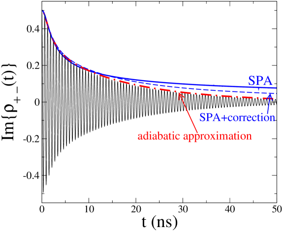
Figure 1: Imaginary part of the coherence $\rho_{+-}(t)$ at $\theta=\pi/2$: Numerical simulations of an adiabatic $1/f$ environment, $S^{1/f}(\omega)\approx[(\pi/4)\,N_{bf}\overline{v^{2}}/\ln(\gamma_{M}/\gamma_{m})]\,\,\omega^{-1}$, correspond to the thin black line. Noise is produced by $n_{d}=250$ bistable fluctuators per decade, with $1/t_{m}=10^{5}$ rad/s $\leq\gamma_{i}\leq\gamma_{M}=10^{9}$ rad/s $<\Omega=10^{10}$ rad/s. The coupling $\bar{v}=0.02\,\Omega$ is appropriate to charge devices, and corresponds to $S(\omega)=16\pi AE_{C}^{2}/\omega$ with $A\sim 10^{-6}$ [36]. The adiabatic approximation fully accounts for dephasing (numerical evaluation of Eq.(14), red dot-dashed line). The Static Path Approximation (SPA) Eq.(17) (blue solid line) and the first correction (blue dashed line) account for the initial suppression, and it is valid also for times $t\gg 1/\gamma_{M}$.

6 Two-qubit universal gate: multi-stage approach

In the present Section we apply the multi-stage approach to a universal two-qubit gate based on a fixed coupling scheme. Capacitive and inductive fixed couplings [39] have been used to demonstrate two-qubit logic gates in different JJ implementations [40]. Entanglement is generated by tuning single-qubit energy spacing to achieve mutual resonance. To this end, during the gate operation at least one qubit has to be moved away from the working point of minimal sensitivity to parameters variations, the ”optimal point”. This has so far represented the main drawback of the fixed-coupling scheme for Josephson implementations, with the exception of phase qubits [41]. More recent proposals have attempted to solve this problem by introducing tunable coupling schemes [42]. Most of them rely on additional circuit elements and gain their tunability from ac-driving [43] or from ”adiabatic” couplers [44]. Some of these coupling schemes have been tested in experiments and are potentially scalable [45]. None of these implementations is however totally immune from imperfections. In general, introducing additional on-chip circuits elements opens new ports to noise. The possibility to employ ”minimal” fixed coupling schemes has been recently reconsidered in Ref. [46], pointing out the possibility to single out ”optimal coupling” conditions which ensure reasonable protection from $1/f$ fluctuations.

In order to implement a $\sqrt{\rm{i-SWAP}}$ gate in a fixed coupling scheme we need two resonant qubits with a transverse coupling, as described by the Hamiltonian

$$\mathcal{H}_{0}=-\frac{\Omega}{2}\,\sigma_{x}^{(1)}\otimes\mathbb{I}^{(2)}-\frac{\Omega}{2}\,\mathbb{I}^{(1)}\otimes\sigma_{x}^{(2)}+\frac{\omega_{c}}{2}\,\sigma_{z}^{(1)}\otimes\sigma_{z}^{(2)}$$ (19)

where $\omega_{c}$ is the coupling strength, and $\sigma_{x}^{(i)}$ the pseudo-spin operators whose eigenstates $|\pm\rangle$ (eigenvalues $\pm 1$) are the computational states of qubit $i$. Eigenvalues and eigenvectors of $\mathcal{H}_{0}$ are given by

$$\omega_{0} = -\Omega\sqrt{1+g^{2}/4}\quad,\quad|0\rangle\,=\,-\sin\frac{\varphi}{2}\,|++\rangle\,+\,\cos\frac{\varphi}{2}\,|--\rangle$$ (20)

$$\omega_{1} = -\omega_{c}/2\quad\quad\;,\quad\quad\quad|1\rangle\,=\,\frac{1}{\sqrt{2}}\,(-|+-\rangle\,+\,|-+\rangle)$$ (21)

$$\omega_{2} = \omega_{c}/2\quad\quad\quad\;,\quad\quad\quad\;|2\rangle\,=\,\frac{1}{\sqrt{2}}\,(|+-\rangle\,+\,|-+\rangle)$$ (22)

$$\omega_{3} = \Omega\sqrt{1+g^{2}/4}\quad\;,\quad\quad|3\rangle\,=\,\cos\frac{\varphi}{2}\,|++\rangle\,+\,\sin\frac{\varphi}{2}\,|--\rangle$$ (23)

where $\sin\varphi=g/(2\sqrt{1+g^{2}/4})$, $\cos\varphi=-1/\sqrt{1+g^{2}/4}$ with $g=\omega_{c}/\Omega$ and we have used the shorthand notation $|\mu\nu\rangle=|\mu\rangle_{1}\otimes|\nu\rangle_{2}\;\mu,\nu\in\{+,-\}$. The level structure of the coupled system is schematically illustrated in Fig.(2). As a result of the diagonal block structure of the Hamiltonian (19) in the computational space, the two-qubit Hilbert space is factorized in two subspaces spanned by pairs of eigenvectors. A system prepared in $|+-\rangle$, freely evolving for a time $t_{E}=\pi/2\omega_{c}$, yields the entangled state $(|+-\rangle-i|-+\rangle)/\sqrt{2}$, corresponding to a $\sqrt{\rm{i-SWAP}}$ operation. The pair of states $|1\rangle$ and $|2\rangle$ span the subspace where the $\sqrt{\rm{i-SWAP}}$ gate is realized, which we name SWAP-subspace. The subspace spanned by the pair of states $|0\rangle$ and $|3\rangle$ is termed Z-subspace.

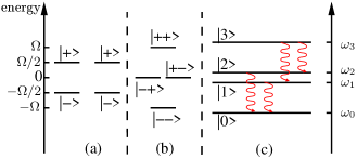
Figure 2: (a) Level structure of the uncoupled resonant qubits; (b) levels in the two-qubit Hilbert space and logic basis of product states. (c) When the coupling is turned on $|+-\rangle$ and $|-+\rangle$ mix and an energy splitting $\omega_{c}\ll\Omega$ develops between the eigenstates $\{|2\rangle,|1\rangle\}$, spanning the SWAP subspace. Product states $|--\rangle$ and $|++\rangle$ weakly mix and split, with $2\Omega\sqrt{1+g^{2}/4}$. The eigenstates $\{|0\rangle,|3\rangle\}$ span the Z subspace. Transverse noise (24) only mix eigenstates belonging to the two subspaces. Dissipative transitions between subspaces are indicated by wavy lines. At typical temperatures, $k_{B}T\ll\Omega$, thermal excitation processes between subspaces can be neglected.

Eq.(19) models, for instance, capacitive coupled charge qubits or inductively coupled flux qubits [40]. Typically, these system can be driven by pulses acting along the transverse direction, $\sigma_{z}^{(i)}$. The same port introduces noise into the system . Here we consider noise sources acting transversely with respect to each qubit, i. e. the interaction Hamiltonian takes the form

$$\mathcal{H}_{\mathrm{I}}=-\frac{1}{2}\,\sigma_{z}^{(1)}\otimes\mathbb{I}_{2}\,\hat{X}_{1}-\frac{1}{2}\,\mathbb{I}_{1}\otimes\sigma_{z}^{(2)}\,\hat{X}_{2}.$$ (24)

Each noise component $\hat{X}_{i}$ has broadband spectrum $S_{X_{i}}(\omega)=\frac{A}{\omega}$, $\omega\in\{\gamma_{m},\gamma_{M}\}$ followed by a white flank at frequencies $\omega\geq\gamma_{M}$. Correlated noise sources acting on both qubits have been addressed in [29].

If the system is initialized in the SWAP subspace, for instance in the state $|+\,-\rangle$, bitwise readout gives the qubit 1 switching probability $P^{(1)}(t)$, i.e. the probability that it will pass to the state $|-\rangle$, and the probability $P^{(2)}(t)$ of finding the qubit 2 in the initial state $|-\rangle$. Cyclic anti-correlation of the probabilities signals the formation of the entangled state during the $\sqrt{\rm{i-SWAP}}$ operation. In terms of the two qubit reduced density matrix in the eigenstate basis the switching probabilities read

$$\!\!\!\!\!\!\!\!\!\!\!\!\!\!\!\!\!\!\!\!\!\!\!\!\!\!\!P^{(1)}(t)=\,\langle-|{\rm Tr}_{2}\rho(t)|-\rangle = \frac{1}{2}\left[\,\rho_{11}(t)+\rho_{22}(t)\right]+\rho_{00}(t)+\left[\,\rho_{33}(t)-\rho_{00}(t)\right]\sin^{2}\frac{\varphi}{2}$$ (25)

$$+{\rm Re}[\rho_{12}(t)]+{\rm Re}[\rho_{03}(t)]\sin\varphi$$

$$\!\!\!\!\!\!\!\!\!\!\!\!\!\!\!\!\!\!\!\!\!\!\!\!\!\!\!P^{(2)}(t)=\langle-|{\rm Tr}_{1}\rho(t)|-\rangle = \frac{1}{2}\left[\,\rho_{11}(t)+\rho_{22}(t)\right]+\rho_{00}(t)+\left[\,\rho_{33}(t)-\rho_{00}(t)\right]\sin^{2}\frac{\varphi}{2}$$ (26)

$$-{\rm Re}[\rho_{12}(t)]+{\rm Re}[\rho_{03}(t)]\sin\varphi.$$

The matrix elements entering the above probabilities can be evaluated in the multi-stage approach.

6.1 Multi-stage approach

We split the interaction as in Eq.(5), $\hat{X}_{i}=\hat{X}_{i}^{Q}+X_{i}(t)$. Low-frequency noise is treated in the adiabatic and longitudinal approximation. In addition we limit the analysis to the SPA. We denote with $\omega_{i}(X_{1},X_{2})$ the eigenvalues of $\mathcal{H}_{0}+\mathcal{H}_{\mathrm{I}}$ with $\hat{X}_{i}\to\{X_{i}\}$.

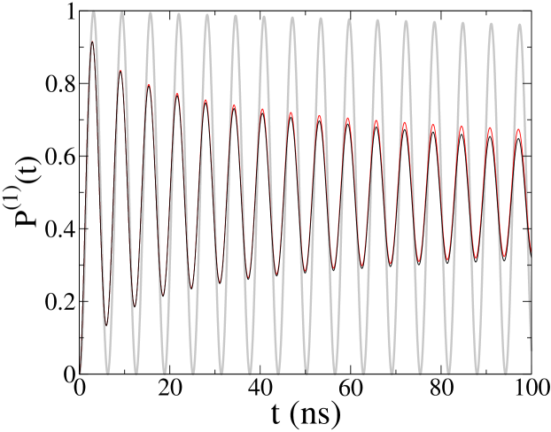
Figure 3: Interplay of adiabatic and quantum noise in the switching probability of qubit 1. Adiabatic noise in the SPA is parametrized by $\sigma/\Omega=0.08$. The effect of low-frequency noise is shown in red, the effect of white noise, $S_{x_{i}}(\omega)\approx 8\times 10^{5}$s^-1, in gray. Interplay of adiabatic and quantum noise is shown by the black line. The interaction strength is $\omega_{c}/\Omega=0.01$.

First stage: elimination of quantum noise Quantum noise is traced out by solving the Born-Markov master equation for the reduced density matrix [49] with eigenvalues parametrically dependent on the random fields $\{X_{i}\}$. In the system eigenstate basis  and performing the secular approximation (to be self-consistently checked) it takes the standard form [27]:

$$\dot{\rho}_{ii}(t) = -\sum_{m\neq i}\Gamma_{im}\,\rho_{ii}(t)+\sum_{m\neq i}\Gamma_{mi}\,\rho_{mm}(t)$$ (27)

$$\dot{\rho}_{ij}(t) = -(i\omega_{ij}+\widetilde{\Gamma}_{ij})\,\rho_{ij}(t)\,,$$ (28)

where $\omega_{ij}=\omega_{i}(X_{1},X_{2})-\omega_{j}(X_{1},X_{2})$. The rates $\Gamma_{lm}$, $\tilde{\Gamma}_{ij}$ depend on the real parts of the lesser and greater Green’s functions, describing emission (absorption) rates to (from) the quantum reservoirs [47]. In addition, for white quantum noise energy shifts are vanishing and do not appear in Eq. (28). Because of the symmetry of (19), dissipative transitions inside each - SWAP or Z - subspace are forbidden. The allowed inelastic energy exchange processes are evidenced in Fig.(2). The only independent emission rates are $\Gamma_{10}=\Gamma_{32}$, $\Gamma_{20}=\Gamma_{31}$. They read

$$\begin{array}[]{ll}\Gamma_{10}=\frac{1}{8}\,(1+\sin\varphi)\,[C_{X_{1}}(\omega_{10})+C_{X_{2}}(\omega_{10})]\\ \Gamma_{20}=\frac{1}{8}\,(1-\sin\varphi)\,[C_{X_{1}}(\omega_{20})+C_{X_{2}}(\omega_{20})]\,,\end{array}$$ (31)

where the absorption rates, $C_{X_{i}}(\omega)=\frac{2\,S_{X_{i}}^{Q}(\omega)}{1+\exp{(-\omega/k_{B}T)}}$, are related to the spectrum of quantum noise, $S_{X_{i}}^{Q}(\omega)$. Emission rates have the same form with $C_{X_{i}}(\omega_{lm})$ replaced by $C_{X_{i}}(-\omega_{lm})$. For the considered initial condition, $|+-\rangle$, the only non vanishing elements of the reduced density matrix in the eigenbasis of ${\mathcal{H}}_{0}$ are the populations and the SWAP coherence, $\rho_{21}(t)$. For independent quantum noise sources acting on the two qubits, the SWAP decay rate reads $\widetilde{\Gamma}_{12}=\frac{1}{2}\,[\Gamma_{10}+\Gamma_{01}+\Gamma_{20}+\Gamma_{02}]=\frac{1}{2}\,[\Gamma_{1}+\Gamma_{2}]$, where $\Gamma_{i}=\Gamma_{i0}+\Gamma_{0i}$, $i=1,2$, are relaxation rates of the SWAP levels. From Eq.(28) we get

$$\rho_{21}(t)=-\frac{1}{2}\,e^{i\omega_{21}(X_{1},X_{2})t}\,e^{-\widetilde{\Gamma}_{12}t}\,.$$ (32)

The secular approximation is valid provided that $\omega_{21}\approx\omega_{c}\gg\widetilde{\Gamma}_{12}$. This condition is fulfilled, for instance, for white noise levels extrapolated from single charge-phase qubit experiments, as it can be evinced from the slow decay due to quantum noise reported in Fig.(3), gray line.

Equations (27) for the populations do not decouple even in the secular limit. General solutions are quite lengthy. Here we report the approximate forms in the small temperature limit with respect to the uncoupled qubits splittings, $k_{B}T\ll\Omega$. In this case level $3$ remains unpopulated and

$$\!\!\!\!\!\!\!\!\!\!\!\!\!\!\!\!\!\rho_{00}(t) \approx 1-\frac{1}{2}[e^{-\Gamma_{20}t}+e^{-\Gamma_{10}t}]\quad,\quad\rho_{11}(t)\approx\frac{1}{2}\,e^{-\Gamma_{10}t}\quad,\quad\rho_{22}(t)\approx\frac{1}{2}\,e^{-\Gamma_{20}t}\,.$$ (33)

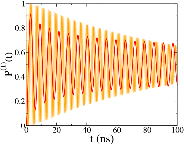
Figure 4: Effect of adiabatic noise under optimal tuning: switching probability of qubit 1 in the presence of low-frequency noise parametrized by $\sigma/\Omega=0.08$ for ”optimal coupling” $\omega_{c}/\Omega=0.08$ (orange) and non-optimal tuning $\omega_{c}/\Omega=0.01$ (red).

Second stage: elimination of adiabatic noise We now consider the effect of low-frequencies in the adiabatic, longitudinal and Static Path approximations. Populations are unaffected by adiabatic noise, whereas the SWAP coherence, $\rho_{12}(t)$, has to be averaged over $X_{i}$. Here we disregard the negligible $X_{i}$ dependence of the rates $\Gamma_{ij}$ via $\omega_{ij}$. Under these simplifying assumption, we are left with the following average

$$\rho_{21}(t)\approx-\frac{1}{2}\,e^{-\widetilde{\Gamma}_{12}t}\,\int dX_{1}dX_{2}\,p(X_{1})p(X_{2})\,e^{i\omega_{21}(X_{1},X_{2})t}.$$ (34)

with $p(X_{i})=\frac{1}{\sqrt{2\pi}\sigma_{i}}\exp{[-\frac{X_{i}^{2}}{2\sigma_{i}^{2}}]}$. The SWAP splitting can be estimated by treating in perturbation theory $\mathcal{H}_{\mathrm{I}}$, with $\hat{X}_{i}\to\{X_{i}\}$, with respect to $\mathcal{H}_{0}$. This leads to

$$\omega_{21}(X_{1},X_{2}) \approx \omega_{c}-\frac{\omega_{c}}{2\Omega^{2}}(X_{1}^{2}+X_{2}^{2})+\frac{\omega_{c}}{8\Omega^{4}}(1+\frac{\omega_{c}^{2}}{\Omega^{2}})(X_{1}^{4}+6X_{1}^{2}X_{2}^{2}+X_{2}^{4})$$ (35)

$$+ \frac{1}{8\omega_{c}\Omega^{2}}(X_{1}^{2}-X_{2}^{2})^{2}.$$

The average in Eq. (34) can be evaluated in analytic form and gives [46]

$$\rho_{12}(t)=-\frac{1}{2}\,e^{-\widetilde{\Gamma}_{12}t}\,\frac{\Omega}{2\sigma^{2}}\sqrt{\frac{2i\omega_{c}}{\pi t}}\,e^{i\omega_{c}t+h(t)}\,K_{0}[h(t)]$$ (36)

where $h(t)=i\omega_{c}/t\,(\Omega^{2}/\sigma^{2}+i\omega_{c}t)^{2}/(4\Omega^{2})$, and $K_{0}[h]$ is the K-Bessel function of order zero [48]. We considered equal standard deviations for noise sources acting on both qubits, $\sigma_{i}\equiv\sigma$. Inserting (33) and (36) in (25) and (26) we obtain the switching probabilities in the multi-stage approach. Out of phase oscillations signals two-qubit states anti-correlations and follows from $P^{({}^{1}_{2})}(t)=P(t)\pm{\rm Re}[\rho_{12}(t)]$, with $P(t)=-\frac{1}{2}\,\cos\varphi\,\left[\rho_{11}(t)+\rho_{22}(t)\right]+\cos^{2}\left(\frac{\varphi}{2}\right)\approx-\frac{1}{4}\,\cos\varphi\,\left[e^{-\Gamma_{10}t}+e^{-\Gamma_{20}t}\right]+g^{2}/4$.

The efficiency of the gate results from the interplay of quantum and adiabatic noise. High-frequency noise levels expected from single qubit experiments [13] weakly affect the switching probability, whose decay is mainly due to low-frequency noise, Fig. (3). Remarkably, considerable recovery of short-times oscillation amplitude may be achieved by an optimal choice of the coupling strength, $\omega_{c}\approx\sigma$ [46]. This regime is illustrated in Fig.(4).

7 Conclusions

In this article we presented a road-map to treat broadband noise typical of solid state nanodevices. The introduced multi-stage approach allows to obtain reasonable approximations by systematically including only the relevant information on the complex environment, out of the huge parametrization which would be required for a microscopic description. Since the environment is in general long-time correlated, the required information depends on the specific protocol.

The predictions obtained with the present approach are in agreement with observations in various single qubit JJ implementations and in different protocols [8, 9]. We extended the procedure to deal with complex solid-state architectures. This is a required step in order to predict efficiency and possibly appropriately design of nanodevices for quantum information processing. Both because of the complexity of architectures and of the unavoidable broadband nature of solid state noise, theoretical tools allowing systematic and controlled approximations are particularly valuable.

As an illustrative case, we performed a simplified analysis of the effects and interplay of low and high frequency noise components in a two-qubit gate in a fixed coupling scheme. Our results points out that efficient operations in the solid state require an accurate preliminary characterization of the noise spectral characteristics and tuning appropriately the device working point.

References

References

- [1] M. Nielsen, I. Chuang, ”Quantum Computation and Quantum Information”, Cambridge Univ. Press, 2005.
- [2] T. Hyashi et al., Phys. Rev. Lett. 91, 226804 (2003); J. R. Petta et al., Phys. Rev. Lett. 93, 186802 (2004); J.R. Petta et al., Science 309, 2180 (2005); J. Gorman, D.G. Hasko, and D.A. Williams, Phys. Rev. Lett. 95, 090502 (2005); F. H. L. Koppens et al., Nature 442, 766 (2006).
- [3] Y. Nakamura et al., Nature 398, 786 (1999); Y. Yu et al., Science 296, 889 (2002); J.M. Martinis et al., Phys. Rev. Lett. 89, 117901 (2002); I. Chiorescu et al., Science, 299, 1869, (2003); T. Yamamoto et al.,Nature 425, 941 (2003); S. Saito et al., Phys. Rev. Lett. 93, 037001 (2004); J. Johansson et al., ibid. 96, 127006 (2006); F. Deppe et al., Nat. Phys. 4, 686 (2008);
- [4] D. Vion et al., Science 296, 886 (2002).
- [5] J. Koch et al. Phys. Rev. A 76, 042319 (2007); J. A. Schreier et al., Phys. Rev. B 77, 180502(R) (2008).
- [6] D. I. Schuster, et al. Nature 431, 162 (2004); D. I. Schuster et al. Nature 445, 515 (2007); M. Göppl et al. Nature 454, 315 (2008); Lev S. Bishop et al. Nature Physics 5, 105 (2008).
- [7] Y. Nakamura et. al, Phys. Rev. Lett. 88, 047901 (2002).
- [8] G. Falci, E. Paladino, R. Fazio, in Quantum Phenomena of Mesoscopic Systems, B. L. Altshuler and V. Tognetti Eds., Proc. of the International School “Enrico Fermi”, Varenna 2002, IOS Press (2003), cond-mat/0312550.
- [9] G. Falci et al., Phys. Rev. Lett. 94, 167002 (2005).
- [10] C. P. Slichter Principles of Magnetic Resonance, Springer-Verlag, Berlin (1996)
- [11] S. Kafanof et al. Phys. Rev. B, 78, 125411 (2008).
- [12] O. Astafiev et al., Phys. Rev. Lett. 93, 267007 (2004).
- [13] G. Ithier et al., Phys. Rev. B 72, 134519 (2005).
- [14] R.W. Simmonds et al., Phys. Rev. Lett. 93, 077003 (2004); K.B. Cooper et al., ibid. 93, 180401 (2004).
- [15] J. Eroms et al., Appl. Phys. Lett. 89, 122516 (2006).
- [16] C. H. Van der Wal, et al., Science 290, 773777 (2000).
- [17] T. Duty et al., Phys. Rev. B 69, 140503(R) (2004);
- [18] Y. M. Galperin et al. Phys. Rev. Lett. 96, 097009 (2006); J Bergli, Y M Galperin and B L Altshuler, New J. Phys. 11, 025002 (2009).
- [19] F. Chiarello private communication 2008. Experiment based on the setup of S.Poletto et al. New J. Phys. 11, 013009 (2008).
- [20] R. Fazio, G. M. Palma, and J. Siewert Phys. Rev. Lett. 83, 5385 (1999).
- [21] M.B. Weissman, Rev. Mod. Phys. 60, 537 (1988).
- [22] J. Claudon et al., Phys. Rev. B 76, 024508 (2007); L. Tian and R.W. Simmonds, Phys. Rev. Lett. 99, 137002 (2007); F. Deppe et al. Phys. Rev. B 76, 214503 (2007); Z. Kim, et al. Phys. Rev. B 78, 144506 (2008); A. Lupascu et al.arXiv:0810.0590.
- [23] A. M. Zagoskin et al. Phys. Rev. Lett. 97, 077001 (2006).
- [24] M. Neeley, et al. Nature Physics 4, 523 (2008).
- [25] E. Paladino et al. Phys. Rev. B 77, 041303(R)(2008).
- [26] S. Ashab et al., New J. Phys. 8, 103 (2006); N. P Oxtoby et al. New J. Phys. 11, 063028 (2009).
- [27] C. Cohen-Tannoudji, J. Dupont-Roc and G. Grynberg Atom-Photon Interactions, Wiley-Interscience (1993).
- [28] E. Paladino et al., Phys. Rev. Lett. 88, 228304 (2002).
- [29] Correlated noise and cross-talk effects have been addressed in A. D’Arrigo et al. NJP 10, 115006 (2008).
- [30] G. Falci et al. in preparation.
- [31] W. Zurek, Physics Today 44, 36 (1991).
- [32] G. M. Palma, K.A. Suominen, A. K. Ekert, Proc. R. Soc. London A, 452, 567 (1996).
- [33] D. G. Cory et al. Phys. Rev. Lett. 81, 2152 (1998).
- [34] C. Isham, Lectures on Quantum Theory: Mathematical and Structural Foundations, Imperial College Press, London (1995).
- [35] Y. Makhlin, A. Shnirman, Phys. Rev. Lett. 92, 178301 (2004).
- [36] A.B. Zorin et al., Phys. Rev. B 53, 13682 (1996).
- [37] Eq. (17) is also valid for Ornstein-Uhlenbeck processes, see [38]. For random telegraph noise the discrete nature of the process modifies this result see E. Paladino et al. Adv. Sol. State Phys., 43, 747 (2003)
- [38] K. Rabenstein, V.A. Sverdlov, D.V. Averin JETP Letters 79, 646 (2004).
- [39] Yu. Makhlin et al., Nature 398, 305 (1999); J. Q. You et al., Phys. Rev. Lett. 89, 197902 (2002).
- [40] Yu. A. Pashkin et al., Nature 421, 823 (2003); A. J. Berkley et al., Science 300, 1548 (2003); T. Yamamoto et al., Nature 425, 941 (2003); R. McDermott et al., Science 307, 1299 (2005); J. B. Majer et al.,Phys. Rev. Lett. 94, 090501 (2005); M. Steffen et al., Science 313, 1423 (2006); J.H. Plantenberg et al., Nature 447, 836 (2007).
- [41] M. A. Sillanpää, J. I. Park and R. W. Simmonds Nature 449, 438 (2007).
- [42] D.V. Averin, C. Bruder, Phys. Rev. Lett. 91, 057003 (2003); A. Blais et al., ibid. 90, 127901 (2003); F. Plastina, G. Falci, Phys. Rev. B 67, 224514 (2003); B.Plourde et al., ibid. 70, 140501(R) (2004); A.O. Niskanen, Y. Nakamura, J.S. Tsai, ibid. 73, 094506 (2006); P. Bertet, C. J. Harmans, J.E. Mooij, ibid. 73, 064512 (2006); Y-D Wang, A. Kemp, K. Semba, ibid. 79, 024502 (2009).
- [43] C. Rigetti, A. Blais, and M. Devoret, Phys. Rev. Lett. 94, 240502 (2005); Yu-xi Liu et al., ibid. 96, 067003 (2006); G. S. Paraoanu, Phys. Rev. B 74, 140504(R) (2006).
- [44] T. V. Filippov et al., IEEE Trans. Appl. Supercond. 13, 1005 (2003); J. Lantz et al., Phys. Rev. B 70, 140507(R) (2004); A. Maassen van den Brink et al., New J. Phys. 7, 230 (2005).
- [45] A. Izmalkov et al., Phys. Rev. Lett. 93, 037003 (2004); M. Grajcar et al., PRB 72, 02503 (2005); T. Hime et al., Science 314, 1427 (2006); A. O. Niskanen et al., Science 316 723 (2007); A. O. Niskanen et al., Nature 447, 386 (2007); J. Majer et al., ibid. 449, 443 (2007); S. H. W. van der Ploeg et al., Phys. Rev. Lett. 98, 057004 (2007); A. Fay et al., ibid. 100, 187003 (2008); A. O. Niskanen et al., Phys. Rev. B 77, 064505 (2008); K. Harrabi et al.,Phys. Rev. B 79, 020507 (2009).
- [46] E. Paladino, A. Mastellone, A. D’Arrigo, G. Falci, arXiv:0906.3115
- [47] U. Weiss, ”Quantum dissipative systems”, Third edition, World Scientific 2008.
- [48] M. Abramowitz, I. A. Stegun “Handbook of Mathematical Functions”, Dover (1965).
- [49] E. Paladino at al. Physica E in press (2009).