Optimization of Planck/LFI on–board data handling

Abstract

To asses stability against $1/f$ noise, the Low Frequency Instrument (LFI) on–board the Planck mission will acquire data at a rate much higher than the data rate allowed by the science telemetry bandwith of 35.5 kbps. The data are processed by an on–board pipeline, followed on–ground by a decoding and reconstruction step, to reduce the volume of data to a level compatible with the bandwidth while minimizing the loss of information. This paper illustrates the on–board processing of the scientific data used by Planck/LFI to fit the allowed data–rate, an intrinsecally lossy process which distorts the signal in a manner which depends on a set of five free parameters ($N_{\mathrm{aver}}$, $r_{1}$, $r_{2}$, $q$, $\mathcal{O}$) for each of the 44 LFI detectors. The paper quantifies the level of distortion introduced by the on–board processing as a function of these parameters. It describes the method of tuning the on–board processing chain to cope with the limited bandwidth while keeping to a minimum the signal distortion. Tuning is sensitive to the statistics of the signal and has to be constantly adapted during flight. The tuning procedure is based on a optimization algorithm applied to unprocessed and uncompressed raw data provided either by simulations, pre–launch tests or data taken from LFI operating in a special diagnostic acquisition mode. All the needed optimization steps are performed by an automated tool, OCA2, which simulates the on–board processing, explores the space of possible combinations of parameters, and produces a set of statistical indicators, among them: the compression rate $C_{\mathrm{r}}$ and the processing noise $\epsilon_{Q}$. For Planck/LFI it is required that $C_{\mathrm{r}}=2.4$ while, as for other systematics, $\epsilon_{Q}$ would have to by less than 10% of rms of the instrumental white noise. An analytical model is developed that is able to extract most of the relevant information on the processing errors and the compression rate as a function of the signal statistics and the processing parameters to be tuned. This model will be of interest for the instrument data analysis to asses the level of signal distortion introduced in the data by the on–board processing. This method was applied during ground tests when the instrument was operating in conditions representative of flight. Optimized parameters were obtained and inserted in the on–board processor and the performance has been verified against the requirements, with the result that the required data rate of 35.5 Kbps has been achieved while keeping the processing error at a level of 3.8% of the instrumental white noise and well below the target 10% level.

 

Remark to the ArXiV version

This is an author-created, un-copyedited version of an article accepted for publication in JINST. IOP Publishing Ltd is not responsible for any errors or omissions in this version of the manuscript or any version derived from it. The present version is derived from the latest version of the paper before final acceptance from JINST, thus it could have some minor differences in phrasing, spelling and style with respect to the published version. The definitive publisher authenticated version is available online at:

http://www.iop.org/EJ/article/-search=68871278.5/1748-0221/4/12/T12018/jinst9_12_t12018.pdf http://www.iop.org/EJ/article/-search=68871278.5/1748-0221/4/12/T12018/jinst9_12_t12018.pdf  

1 Introduction

One of the most challenging aspects in the design of an astronomy mission in space is the ability to send the collected data to the ground for the relevant analysis within the allowable telemetry bandwidth. In fact the increasing capabilities of on–board instruments generates ever larger ammounts of data whereas the downlink capability is quite constant being mainly governed by the power of the on–board transmitter and the length of the time window which can be allocated for data down linking [Bertotti, Farinella, Vokrouhlický (2003)]. In the case of the ESA satellite Planck, which will observe the CMB from the second Lagrangian point (L2) of the Earth – Sun system, $1.5\times 10^{6}$ Km far from Earth, the down–link rate is limited to about 1.5 Mbps, and Planck can be in contact with the ground station (located at New Norcia, Western Australia) for no more than a couple of hours each day thus reducing the effective bandwidth by an order of magnitude. In addition, Planck carries two scientific instruments: the Planck Low Frequency Instrument (Planck/LFI), to which this paper is devoted, and the Planck High Frequency Instrument (Planck/HFI). Both share the bandwidth to download data with other internal spacecraft services and the up–link channel The result is that LFI has only about 53.5 Kbps average down link rate while producing a unprocessed data rate of about 5.7 Mbps. It is evident that some kind of on–board data compression must be applied to fit in to the available telemetry bandwidth.

It is well known that the theoretical maximum compression rate achievable for a given data stream decreases with its increasing variance. Thus it is very advantageous before appying any compression algorithm to preprocess the data to reduce its inherent variance. In the ideal case the preprocessing would not alter the original data, but in practice some information loss can not be avoided when the variance is reduced. Thus the on–board preprocessing algorithm should be tunable through some kind of free processing–parameters in order to asses at the same time the required compression rate at the cost of a minimal degradation of the data. This paper addresses the problem of the on–board processing and the corresponding ground processing of the scientific data and the impact on its quality for the Planck/LFI mission. This has also been the topic of two previous papers, the first regarding the exploration of possible lossless compression strategies [Maris et al. (2000)], and the second focused to the assessment of the distortions introduced by a simplified model of the on–board plus on–ground processing [Maris et al. (2004)]. Here the work presented by [Maris et al. (2004)] is completed by introducing in Sect. 2 a brief description of the instrument followed by a quantitative model of the on–board plus on–ground processing applied in Planck/LFI. The processing can be tuned with the statistical properties of the signal and introduce as small as possible distortion. to asses the proper compression rate and as small as possible processing distortion. This can be performed by using a set of control parameters, as anticipated in [Maris et al. (2004)], which are tuned on the real signal. The tuning algorithm, which has not been discussed previously, is the most important contribution to the Planck/LFI programme presented in this work and it is discussed in Sect. 3. The whole procedure has been validated both with simulations and during the pre–flight ground testing. The most signifcative results are reported in Sect. 4. Of course, processing has an impact on Planck/LFI science whose complete analysis is outside the scope of this paper but however is briefly analyzed in Sect. 5. At last Sect. 6 reports the final remarks and conclusions, while some technical details are presented in appendices A, B and C.

2 Radiometer model and acquisition chain

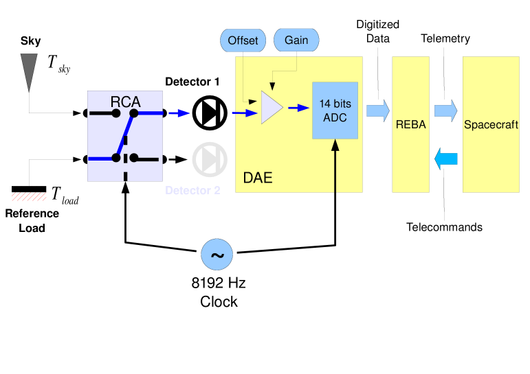
Figure 1: A schematic view of the main flow of scientific data for a single RCA of Planck/LFI. Each RCA has two detectors, but in this scheme only the first is represented and schematized. For graphical purposes the scheme represents just the first detector while connected to the reference–load, while Detector 2 would be connected to sky. At a change of the Clock phase the two detectors will switch their connections. The block arrows represents the flow of digitized data and telemetry toward the spacecraft and the flow of telecommands from the spacecraft.

Planck/LFI [Bersanelli et al. (2009)] is based on an array of 22 radiometers assembled in 11 Radiometric Chain Assemblies (RCA) in the Planck focal plane. Each RCA has 4 radio frequency input lines and 4 radio frequency output lines, hence the number of radio frequency outputs to be measured by the on–board electronics is 44. Each feed–horn has one orthomode transducer with two outputs: each extracting the two orthogonal components of linear polarization in the signal received from the sky and feeding one of the radio frequency input lines of a radiometer, the other radio frequency input line is connected to a reference–load held at the constant temperature of 4.5 K.

A schematic representation of the flow of information in a single radiometer belonging to a RCA is given in Fig. 1. Each radiometer acts as a pseudo–correlation receiver [Villa et al. (2009)] measuring the difference in antenna temperatures, $\Delta T$, between the sky signal, ${T_{\mathrm{sky}}}$, and the reference–load  ${T_{\mathrm{load}}}$, [Valenziano at al.(2009)]. However, given the sky and the reference–load have different mean temperatures the reference samples have to be scaled by a Gain Modulation Factor, $r$, which balances the difference between ${T_{\mathrm{sky}}}$ and ${T_{\mathrm{load}}}$ to a $\mathrm{mean}{\left[\Delta T\right]}=0$ so that

$$\Delta T={T_{\mathrm{sky}}}-r{T_{\mathrm{load}}}.$$ (1)

A proper choice of $r$ will allow near cancellation out most of the first order systematic errors [Mennella et al. (2003), Mehinold at al.(2009)], assuring in this way optimal rejection of systematics, in particular drifts and the $1/f$ noise [Mennella et al. (2009)]. As a first approximation it is possible to put

$$r\approx\frac{\mathrm{mean}{\left[{T_{\mathrm{sky}}}\right]}+{T_{\mathrm{noise}}}}{\mathrm{mean}{\left[{T_{\mathrm{load}}}\right]}+{T_{\mathrm{noise}}}},$$ (2)

where ${T_{\mathrm{noise}}}$ is the noise temperature. Eq. (2) makes evident how different values of $r$ are needed in the various phases of the mission. In particular three cases are important: ground tests, in–flight cooling phase and finally in–flight operations with the instrument in nominal conditions. As an exemple consider the case of the 30 GHz channel, which is the least noisy channel of Planck/LFI having an expected ${T_{\mathrm{noise}}}\approx 10$ K. During on–ground testing $\mathrm{mean}{\left[{T_{\mathrm{sky}}}\right]}\approx\mathrm{mean}{\left[{T_{\mathrm{load}}}\right]}$ and so $r\approx 1$ ([Bersanelli et al. (2009), Mennella et al. (2009)]). In flight $\mathrm{mean}{\left[{T_{\mathrm{sky}}}\right]}\approx 2.725$ K but during the cooling $\mathrm{mean}{\left[{T_{\mathrm{load}}}\right]}$ varies from $\approx 20$ K down to the nominal $\mathrm{mean}{\left[{T_{\mathrm{load}}}\right]}\approx 4.5$ K. Thus $r$ varies from $\approx 0.4$ when the instrument starts to cool–down to $\approx 0.88$ at the end of the process when it reaches its nominal temperature. With higher values of ${T_{\mathrm{noise}}}$ the other channels will show smaller departures in their $r$ from 1 as well as a lower sensitivity to the environmental conditions.

To acquire sky and reference–load signals each radiometer has two separate radio frequency inputs, and correspondingly two radio frequency outputs, each one connected to a radio frequency detector and to an acquisition chain ending in a 14 bit analog–to–digital converter (ADC) housed in the Digital Acquisition Electronics box (DAE) [Bersanelli et al. (2009), Villa et al. (2009)]. The output of the DAE is sent to the Radiometer Electronics Box Assembly box (REBA) which processes the data from the DAE, of interpreting and executing telecommands, and of interfacing the instrument with the spacecraft Central Data Management Unit. This unit produces the scientific packets to be sent to the ground [Herreros et al. (2009)].

The DAE applies a individually programmable analogue offset to each input signal prior to applying individual programmablt gains and performing digitization. The contribution to the read–out noise budget from the ADC quantization is in general considered marginal. Appendix B discusses the case in which this hypothesis is no longer valid. The offset and the gain are adjustable parameters of the DAE and it is assumed that their calibration is independent from the REBA calibration [Cuttaia at al.(2009)] with an exception which is discussed in Appendix C. The ADCs are fetched in turn and the data are sent to the Science Processing Unit (SPU), a Digital Signal Processor (DSP) based computer which is part of the REBA [Herreros et al. (2009)] not represented in Fig. 1. The SPU stores the data in circular buffers for subsequent digital processing and and then applies the on board software pipeline to the data, In the process the 14 bit single samples are convert to 16 bits signed integers. The content of each ADC buffer is processed separately by the on–board processing pipeline and sent to ground.

As usual in these kinds of receivers, the required stability of the radiometers is assured by switching each radiometer between the sky and reference–load. Thus each output alternatively holds the sky and the reference–load signal (or the reference–load and the sky) with opposed phases between the two channels. Hence, each buffer contains strings of interlaced sky—-reference–load (or reference–load—-sky) samples in increasing order of acquisition time, $t$ i.e.

$$T^{\mathrm{ADC}}_{\mathrm{sky},t=0},T^{\mathrm{ADC}}_{\mathrm{load},t=1},T^{\mathrm{ADC}}_{\mathrm{sky},t=2},T^{\mathrm{ADC}}_{\mathrm{load},t=3},\dots,$$ (3)

or

$$T^{\mathrm{ADC}}_{\mathrm{load},t=0},T^{\mathrm{ADC}}_{\mathrm{sky},t=1},T^{\mathrm{ADC}}_{\mathrm{load},t=2},T^{\mathrm{ADC}}_{\mathrm{sky},t=3},\dots.$$ (4)

The switching frequency is fixed by the LFI internal clock at $8192~{}\mbox{Hz}$. The switch clock gives also the beat for the ADCs, which are then synchronized with the switching output, and it is sensed by the on-board processor, which uses it to reconstruct the ordering of the signals acquired from the ADCs and to synchronize it with the on–board time. This frequency also synchronises the ADCs with the input and is used by the SPU to reconstruct the ordering of the signals acquired from the ADCs and to synchronise them with the on board time.

The data flow of raw data is equivalent to 5.7 Mbps; a large amount of data that cannot be fully downloaded to the ground. The allocated bandwidth for the instrument is equivalent to only 53.5 kbps including all the ancillary data, less than 1% of the overall data generated by LFI. The strategy, adopted to fit into the bandwidth, relies on three on–board processing steps, downsampling, preprocessing the data to ensure lossless compression, and lossless compression itself. To demonstrate these steps, a model of the input signal shall be used. It has to be noted that while the compression is lossless, the preprocessing is not, due to the need to rescale the data and convert them in integers, (a process named data requantizzation). However, the whole strategy is designed to asses a strict control of the way in which lossy operations are done, of the amount of information loss in order to asses optimal compression rate with minimal information loss.

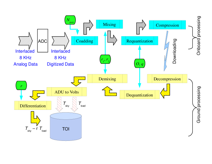
Figure 2: Schematic representation of the scientific onboard and ground processing for the Planck/LFI. Cyan boxes represent REBA operations, yellow boxes ground operations. Green pads specify the parameters needed by each operation. TOI could be produced both in undifferentiated form (${T_{\mathrm{sky}}}$, ${T_{\mathrm{load}}}$ stored separately) or in differentiated form.

2.1 Signal model

We describe quantitatively the kind of signal the pipeline has to process by modeling the output of the DAE as a function of time, $t$, as

$${T_{\mathrm{sky}}}(t) = \overline{T}_{\mathrm{sky}}+\Delta T_{\mathrm{sky}}(t)+{n_{\mathrm{sky}}},$$ (5)

$${T_{\mathrm{load}}}(t) = \overline{T}_{\mathrm{load}}+\Delta T_{\mathrm{load}}(t)+n_{\mathrm{load}}.$$ (6)

where $\overline{T}_{\mathrm{sky}}$, $\overline{T}_{\mathrm{load}}$ are the constant part of the signal. $\Delta T_{\mathrm{sky}}$, and $\Delta T_{\mathrm{load}}$ a possible deterministic time dependent parts, representing drifts, dipoles, oscillations and so on, ${n_{\mathrm{sky}}}$ and $n_{\mathrm{load}}$ represents the random noise whose moments are $\sigma_{n,\mathrm{sky}}^{2}$, $\sigma_{n,\mathrm{load}}^{2}$, and whose covariance is $\sigma_{n,\mathrm{sky},\mathrm{load}}$.

The pipeline described in the following sections needs to be tuned to obtain a proper level of data compression which is largely determined by the covariance matrix of the signal whose components are

$$\sigma_{\mathrm{sky}}^{2} = \mathrm{var}{\left[\Delta T_{\mathrm{sky}}\right]}+\sigma_{n,\mathrm{sky}}^{2}$$ (7)

$$\sigma_{\mathrm{load}}^{2} = \mathrm{var}{\left[\Delta T_{\mathrm{load}}\right]}+\sigma_{n,\mathrm{load}}^{2}$$ (8)

$$\sigma_{\mathrm{sky},\mathrm{load}} = \mathrm{cov}{\left[\Delta T_{\mathrm{sky}},\Delta T_{\mathrm{load}}\right]}+\sigma_{n,\mathrm{sky},\mathrm{load}}$$ (9)

where it has been assumed that the random and deterministic parts are uncorrelated. It is useful to identify two extreme cases: the data stream is signal dominated, when $\mathrm{var}{\left[\Delta T_{\mathrm{sky}}\right]}+\mathrm{var}{\left[\Delta T_{\mathrm{load}}\right]}\gg\sigma_{n,\mathrm{sky}}^{2}+\sigma_{n,\mathrm{load}}^{2}$, or the data stream is noise dominated, when $\mathrm{var}{\left[\Delta T_{\mathrm{sky}}\right]}+\mathrm{var}{\left[\Delta T_{\mathrm{load}}\right]}\ll\sigma_{n,\mathrm{sky}}^{2}+\sigma_{n,\mathrm{load}}^{2}$. In the noise dominated case, the statistics of data will be largely determined by the statistics of noise, which in general could be considered normally distributed and uncorrelated over short time scales, given the $1/f$–noise will introduce correlations over long time scales. In the signal dominated case the statics of data will be instead determined by the kind of time dependence in the signal. As an example, if $|\overline{T}_{\mathrm{sky}}-\overline{T}_{\mathrm{load}}|$ is large compared to the noise while $\Delta T_{\mathrm{sky}}$ and $\Delta T_{\mathrm{load}}$ are negligible, the histogram of the signals will resemble the sum of two Dirac’s delta functions $\delta(x-\overline{T}_{\mathrm{sky}})+\delta(x-\overline{T}_{\mathrm{load}})$ convolved with the distribution of noise.

If a linear time dependence of the kind $\Delta T(t)=\dot{A}t+C$ is present, then the distribution of the samples will be uniform and bounded between $\overline{T}\pm\dot{A}\tau/2$, where $\tau$ is the time interval relevant for the signal sampling. The variance will be $A_{\tau}^{2}/12$ where $A_{\tau}=\dot{A}\tau$ is the drift amplitude over the time scale $\tau$. The signal could be considered noise dominated if $\tau<\sqrt{12}\sigma/|\dot{A}|$. From the point of view of data compression, in determining whether a signal is noise dominated or not, the critical factor is the time scale $\tau$. For our coupled signals, denoting with ${\dot{A}_{\mathrm{sky}}}$ and $\dot{A}_{\mathrm{load}}$ the drift rate in the sky and reference–load signals, and with $A_{\mathrm{sky},\tau}$, $A_{\mathrm{load},\tau}$ the relative amplitudes, the relevant components of the covariance matrix will be

$$\mathrm{var}{\left[\Delta T_{\mathrm{sky}}\right]}_{\tau}=\frac{A_{\mathrm{sky},\tau}^{2}}{12}$$ (10)

$$\mathrm{var}{\left[\Delta T_{\mathrm{load}}\right]}_{\tau}=\frac{A_{\mathrm{load},\tau}^{2}}{12}$$ (11)

$$\mathrm{cov}{\left[\Delta T_{\mathrm{sky}},\Delta T_{\mathrm{load}}\right]}_{\tau}=\frac{A_{\mathrm{sky},\tau}A_{\mathrm{load},\tau}}{12}$$ (12)

In this regard, the most important $\tau$ to be considered in this work is the time span for the chunk of data contained in a packet, which is the minimum unit of formatted data sent by the REBA to the ground. Each scientific packet produced by the REBA has a maximum size corresponding to 1024 octects, part of which has to be allocated for headers carring ancillary informations such as the kind of data in the packet or the time stamp. So, even taking into account data compression, only a small amount of data can be stored in a packet corresponding to about $6-22$ secs, which depends on details such as the attained compression rate and the frequency channel involved, as will be shown in Sect 2.3. More complicated distributions may occur for a polynomial time dependence of the kind $\Delta T\propto t^{n}$, or for a sinusoidal time dependence of period $P$: $\Delta T\propto sin(2\pi t/P)$, but in most cases a simple linear drift $\Delta T\propto t$ could be taken as a reference model given that non periodic drifts are bounded in amplitude by corrective actions commanded from the ground station, while periodic variations have periods much longer than the time span of a packet. Also in general it is assumed that the mean $\mathrm{mean}{\left[\Delta T_{\mathrm{sky}}\right]}=0$ and the $\mathrm{mean}{\left[\Delta T_{\mathrm{load}}\right]}=0$ but it is interesting to discuss even the case in which this is not strictly true.

2.2 Data compression and on–board processing

The strategy adopted to remain inside the downlink bandwidth is based on three processing steps: i) signal downsampling, ii) signal conditioning and entropy reduction, iii) loss-less compression [Bersanelli et al. (2009), Miccolis (2003)]. A schematic representation of the sequence in which these steps are applied on–board and whenever possible reversed on–ground is given in Fig. 2. The figure refers to a single radiometer chain and is ideally splitted into two parts: the upper part depicts the on–board processing with cyan boxes denoting the main steps. The corresponding on–ground processing is depicted in the lower part with the main steps coloured in yellow. Green pads represents the processing parameters. The first four of them are refered to as REBA parameters, and they are applied both on–board and on–ground. The parameters are: the number of ADC raw samples to be coadded to form an instrumental sample, $N_{\mathrm{aver}}$, the two mixing parameters $r_{1}$, $r_{2}$, the offset $\mathcal{O}$ to be added to data after mixing and prior to requantization, and the requantization step $q$. The exact meaning of each of these parameters will be explained later in the text, when each step will be explained in full detail. It is important to recall that the on–board parameters are imposed by telecommands sent from the ground. They are copied in each packet carring scientific data and on–ground they are recovered from the packets to be applied by the on–ground processing. The $r$ factor is a parameter of the ground processing and is computed from the total power data received on the ground. The final products in the form of Time Ordered Data (TOI) either in total power or differentiated are stored in an archive represented by the light–blue cylinder.

Before entering into the details of the various steps it has to be noted that in principle a factor of two compression would be immediately gained by directly computing the difference between sky and reference–load on–board, i.e. sending differentiated data at Earth. Although on–board differentiation seems straightforward , it implies at least a couple of major disadvantages. First, once the difference is made, separate information about the sky and the reference–load is lost, preventing an efficient detection and removal of other many second order systematics. Second a set of 44 $r$ factors could be in principle easily uploaded on–board and applied to the data, but the $r$ for each detector has to be fine–tuned on the real data. This would mean that the optimal $r$ should be continuously monitored and adjusted to avoid uncontrolled drifts for each radiometer, but this is inpractical, having just 3 hours of connection per day. In addition, an error in calibrating the $r$ will cause an irremediable loss of data. Therefore, the best solution is to downlink the sky and the reference–load samples separately allowing the application on the ground of the optimal $r$.

2.3 Downsampling

Each sky sample contains the sky signal integrated over a sky area as wide as the beam, but since each radiometer is sampled at a frequency of 8192 Hz the sky is sampled at an apparent resolution of about $1/2$ arcsec. On the other hand the beam size for each radiometer goes from 14 arcmin for the 70 GHz to 33 arcmin for the 30 GHz. Consequently it is possible to co–add $N_{\mathrm{aver}}$, consecutive samples producing averaged samples whose sampling time correspond to a more reasonable resolution without any loss of information.

1. The downsampling algorithm takes $N_{\mathrm{aver}}$ couples of sky—-reference–load (reference–load—-sky) samples from a given ADC; 2. separates the two subsets of signals; 3. computes the sum of sky and load subsets (represented by 32–bits signed integers); 4. interlaces them; and 5. stores them as sky—-reference–load (reference–load—-sky) couples in an circular buffer for subsequent processing. In normal processing the REBA converts these sums into averages by converting them into floating–point format and then dividing them by $N_{\mathrm{aver}}$ prior to perfom the subsequent steps of mixing, requantization and compression. In the case of diagnostic data processing the REBA transfers directly as output these sums as they are i.e. without any other processing or compression. In this case the ground–segment pipeline has the task of converting them into averages. This is a trade–off between the need for packets to carry just data represented by 16 or 32 bits integers, and the need to avoind uncontrolled round–off errors in the conversion of floating–point averages in integer values. Note that the diagnostic telemetry is very limited in flight by telemetry bandwith.

The value of $N_{\mathrm{aver}}$ depends on the beam–width, $b_{\mathrm{rad}}$, for the given detector

$$N_{\mathrm{aver}}=\frac{\omega_{\mathrm{spin}}n_{\mathrm{over}}\sin\beta}{b_{\mathrm{rad}}f_{\mathrm{sampling}}}$$ (13)

$\omega_{\mathrm{spin}}$ [rad/sec] is the rate at which the satellite spins about its spin axis [The Planck Bluee Book (2005), Dupac, Tauber (2005), Maris et al. (2005)], $\beta$ is the boresight angle between the telescope line–of–sight and the spin axis, and $n_{\mathrm{over}}=3$ is the the number of samples per beam. Nominal values for the $N_{\mathrm{aver}}$ are 126, 88, 53 respectively for the 30 GHz, 44 GHz and 70 GHz frequency channels. The corresponding sampling frequencies in the sky are then 65 Hz, 93.1 Hz and 154.6 Hz, while samples are produced at a rate twice the sampling frequency. This drastically reduces the data rate that becomes about 85 kbps without introducing an important loss in scientific information.

The output of the downsampling stage can be seen as a sequence of sky—-reference–load couples ordered according to the generation time $t$

$$\left(\begin{array}[]{c}{T_{\mathrm{sky}}}\\ {T_{\mathrm{load}}}\end{array}\right)_{t=0},\left(\begin{array}[]{c}{T_{\mathrm{sky}}}\\ {T_{\mathrm{load}}}\end{array}\right)_{t=\delta_{t}},\left(\begin{array}[]{c}{T_{\mathrm{sky}}}\\ {T_{\mathrm{load}}}\end{array}\right)_{t=2\delta_{t}},\dots,\left(\begin{array}[]{c}{T_{\mathrm{sky}}}\\ {T_{\mathrm{load}}}\end{array}\right)_{t=n\delta_{t}},\dots$$

where $\delta_{t}=2N_{\mathrm{aver}}/f_{\mathrm{sampling}}$ the samples are interlaced to generate a string of time ordered samples as

$${T_{\mathrm{sky}}}_{,0},{T_{\mathrm{load}}}_{,0},{T_{\mathrm{sky}}}_{,\delta_{t}},{T_{\mathrm{load}}}_{,\delta_{t}},{T_{\mathrm{sky}}}_{,2\delta_{t}},{T_{\mathrm{load}}}_{,2\delta_{t}},\dots,{T_{\mathrm{sky}}}_{,n\delta_{t}},{T_{\mathrm{load}}}_{,n\delta_{t}},\dots$$

in a manner similar to the output of the ADC. But, while sky and reference–load samples in each ADC output buffer are consecutive in time, this is no longer true for the downsampled values. As an example, assuming a sequence from the ADC where even samples are $T^{\mathrm{ADC}}_{\mathrm{sky}}$ and odd samples are $T^{\mathrm{ADC}}_{\mathrm{load}}$ (i.e., ${T_{\mathrm{sky}}}$, ${T_{\mathrm{load}}}$ sequences), then any ${T_{\mathrm{sky}}}_{t}$ will be the sum of $N_{\mathrm{aver}}$ samples with times between $t$ and $t+2(N_{\mathrm{aver}}-1)/f_{\mathrm{sampling}}$ while and ${T_{\mathrm{load}}}_{t}$ will span the time range $t+1/f_{\mathrm{sampling}}$ and $t+2N_{\mathrm{aver}}/f_{\mathrm{sampling}}$. While this small time shift is not very important when observing sky sources, it might be relevant when attempting to correlate the observed signal with internal sensors, such as those used to determine the level of perturbation introduced by the active cooling. However, this problem is probably more theoretical than real as internal temperature variations do not occur on very small timescales. For simplicity, in the remainder of the text we will omit to specify time in our formulas.

2.4 Lossless compression, packeting and processing error

To better understand the intermediate step of processing, i.e. mixing and requantization, it is necessary to introduce here the last step of lossless compression. The familiar technique of lossless compression is based on the ability of the compression software to recode a stream of symbols by using codewords which on average are shorther than those used in input, and in a way which could be fully recovered on ground by a decompression code. The coding for the data stream in output to the compressor has to be optimized by taking into account the statistical distributions of the symbols in the input data stream. For this reason, lossless compressors maintain an internal representation of the data distribution, such as the histogram or similar statistical indicators. In our case the selected compression scheme is based on a 16–bit, zero order, adaptive arithmetic entropy encoder [Herreros et al. (2009)]. The compressor assumes that the data stream is represented by an uninterrupted list of couples of 16–bit integers. It does not take any particular interpretation of the content of the samples or of the order in which they are presented. It simply keeps coding and storing data in the packet until the maximum length is reached. The packet is then closed and a new packet is opened. The compressor uses an adaptive scheme to decide the best coding for the input data as they are produced by the previous steps of the on–board pipeline. On ground the decompressor extracts the samples from each packet in the same order in which they have been introduced by the compressor. In this sense the compressor/decompressor couple act as a First In – First Out device, and becomes nearly transparent in the scientific processing of the data.

The basic requirement for the packets produced by the compression stage is that of packet independency i.e. it must be possible to interpret the content of each packet independently of all the others. For LFI it means that the pipeline in the ground segment shall be allowed to generate from each single packet chunks of differentiated data. So the compressor must store consecutive couples of sky—-reference–load samples within each packet together with the information needed by the decompressor to interpret the compressed packets. In addition the compressor must be able to self–adapt its coding scheme to the statistics of the input signal, without the need of any prior information on it. Finally, the compressor must be fast enough to allow real–time elaboration of data with limited memory consumption. These requirements suggest the use of a compression scheme in which the compressor updates its internal statistical table each time it receives a sample. An empty statistical table is then imposed at the beginning of the compression of a new packet, therefore assuring complete independence. When a symbol not present in the table is received as input a pseudo–symbol corresponding to a “stop message” is issued, followed by the uncompressed new symbol, after that the internal statistical table is updated. If the symbol is in the table, the corresponding entry is updated and the symbol is coded accordingly. On ground the decompressor starts with the same empty internal statistical representation assuming the first symbol is a stop followed by a new symbol, and it updates the table accordingly as it receives symbols to decode or stop symbols.

The efficiency of a compressor is typically measured by the, so called, compression rate $C_{\mathrm{r}}$ defined as the ratio between the length of an output string $L_{\mathrm{out}}$ derived from the compression of an input string of length $L_{\mathrm{in}}$

$$C_{\mathrm{r}}=\frac{L_{\mathrm{out}}}{L_{\mathrm{in}}}.$$ (14)

Of course, to accomodate a given data rate $R_{\mathrm{data}}$ inside a given bandwidth $B_{\mathrm{data}}$ a target compression rate has to be obtained leading to the obvious definition

$$C_{\mathrm{r}}^{\mathrm{Tgt}}=\frac{R_{\mathrm{data}}}{B_{\mathrm{data}}}.$$ (15)

It is well known that any lossless compressor based on entropy encoding has an upper limit for the highest compression rate

$$C_{\mathrm{r}}^{\mathrm{Th}}=\frac{N_{\mathrm{bits}}}{H},$$ (16)

where $N_{\mathrm{bits}}$ is the number of bits used for coding the samples and $H$ is Shannon’s entropy for the signal, which in turns depends on its probability distribution function (PDF). For an optimal compressor the theoretical $C_{\mathrm{r}}^{\mathrm{Th}}$ for a digitized signal represented by integers in the range $Q_{\mathrm{min}}\leq Q\leq Q_{\mathrm{max}}$ is given by

$$C_{\mathrm{r}}^{\mathrm{Th}} = \frac{N_{\mathrm{bits}}}{H},$$ (17)

$$H = -\sum_{Q=Q_{\mathrm{min}}}^{Q_{\mathrm{max}}}f_{Q}\log_{2}f_{Q}:$$ (18)

where $H$ is the Shannon entropy for the data stream, $f_{Q}$ is the frequency by which the symbol or value $Q$ occurs in the data stream, having $\lim_{f_{Q}\rightarrow 0}f_{Q}\log_{2}f_{Q}=0$, and $\sum_{Q=Q_{\mathrm{min}}}^{Q_{\mathrm{max}}}f_{Q}=1$. Non–idealities in the signal and in the compressor cause the effective $C_{\mathrm{r}}$ to be different from the expected $C_{\mathrm{r}}^{\mathrm{Th}}$ having $C_{\mathrm{r}}^{\mathrm{Th}}>C_{\mathrm{r}}$. Usually this is accounted for by scaling $C_{\mathrm{r}}^{\mathrm{Th}}$ by a multiplicative efficiency factor $\eta$. However its exact determination is a complex task described in some detail in Sect. 3.4 and for the time being we will neglect it.

From Eq. (17) and (18), to maximize $C_{\mathrm{r}}$ we need to minimize $H$ for the input signal, forcing the reduction of its variance by requantizing the data. I.e. dividing the data by a quantization step, $q$, and rounding off the result to the nearest integer

$$Q=\mathrm{round}\left(\frac{X+\mathcal{O}}{q}\right),$$ (19)

where $\mathcal{O}$ is an additive constant usually defined by asking

$$\mathrm{mean}{\left[X+\mathcal{O}\right]}=0.$$ (20)

On ground the data are then decompressed and reconstructed by multiplying them by $q$.

$$\tilde{X}=q[Q-\mathcal{O}].$$ (21)

Some information is lost in the process and causes a processing distortion, $\epsilon_{q}$, which in the simplest case is approximated by

$$\epsilon_{q}=\mathrm{rms}{\left[\tilde{X}-X\right]}\approx\frac{q}{\sqrt{12}}.$$ (22)

In [Maris et al. (2000), Maris et al. (2004)] we studied the case $X=\Delta T$, there it had been shown that for Planck/LFI the statistics of the differentiated data stream was approximated by a nearly univariate normal distribution with $\sigma=\mathrm{rms}{\left[\Delta T\right]}$, and that after re quantization and reconstruction both $C_{\mathrm{r}}^{\mathrm{Th}}$ and $\epsilon_{q}$ where largely parameterized by the $\sigma/q$ ratio with

$$C_{\mathrm{r}}^{\mathrm{Th}} \approx \frac{N_{\mathrm{bits}}}{\log_{2}\left(\sqrt{2\pi e}\frac{\sigma}{q}\right)};$$ (23)

$$\frac{\epsilon_{q}}{\sigma} \approx \frac{1}{\sqrt{12}}\left(\frac{\sigma}{q}\right)^{-1};$$ (24)

of course we need to assure that ${\epsilon_{q}}/{\sigma}<1$ which is expected to be satisfied “by design” for Planck/LFI. In this regard, it has to be recalled how the limit to any instrumental residual error for Planck/LFI was assessed in the context of the overall error budget (including thermal, radiometric, optical and data-handling effects), driven by the ultimate requirement of a cumulative systematic error per pixel smaller than $3\;\mu\mathrm{K}$ (peak–to–peak) at the end of the mission. The 10% limit for the on–board processing-related errors has been set as a reachable requirement which should lead to a nearly-negligible impact on science.

We are now in the position of deriving the expected time spans for the compressed chunks of data contained in Planck/LFI packets which have been reported at the end of Sect. 2.1. It is sufficient to consider that each packet may carry a maximum number $\mathcal{N}_{\mathrm{smp}}$ of $N_{\mathrm{bits}}$ code–words representing scientific data, each representing on average $C_{\mathrm{r}}^{\mathrm{Tgt}}$ samples either sky or reference–load and that the sampling period after the downsampling is $f_{\mathrm{sampling}}/N_{\mathrm{aver}}$ to obtain

$$\tau_{\mathrm{pck}}\approx\frac{2N_{\mathrm{aver}}\mathcal{N}_{\mathrm{smp}}C_{\mathrm{r}}^{\mathrm{Tgt}}}{f_{\mathrm{sampling}}},$$ (25)

where the factor of $2$ in front of $N_{\mathrm{aver}}$ comes from the fact that the sky-reference–load cycle has half the frequency of the ADC sampling. For Planck/LFI $\mathcal{N}_{\mathrm{smp}}=490$, while a $C_{\mathrm{r}}^{\mathrm{Tgt}}=2.4$ would be sufficient to allow proper data compression. Of course, some level of variability among the detectors has to be allowed in order to cope with non stationarities in the time series, or with the need to share the bandwidth among different detectors in different manners. So a good fiducial range of values for $C_{\mathrm{r}}^{\mathrm{Tgt}}$ for individual detectors is $2<C_{\mathrm{r}}^{\mathrm{Tgt}}<3$, leading the expected values for $\tau_{\mathrm{pck}}$ to vary over $15-22$ sec, $10-16$ sec and $6-9$ sec respectively for the 30 GHz, 44 GHz and 70 GHz frequency channels.

2.5 The mixing algorithm

In general a data stream made of alternate sky and reference–load samples can not be approximated by a normal, univariate distribution. Two different populations of samples, with different statistical properties are mixed together. In this case the $C_{\mathrm{r}}$ could be reduced with respect to the univariate case. Furthermore, most of the first order instabilities, such as drifts and $1/f$–noise, come from the radiometers, produces spurious correlated signals in ${T_{\mathrm{sky}}}$ and ${T_{\mathrm{load}}}$. For these reasons undifferentiated time–lines for ${T_{\mathrm{sky}}}$ and ${T_{\mathrm{load}}}$ are much more unstable than the corresponding $\Delta T$ timelines further reducing $C_{\mathrm{r}}$. In particular, fast drifts may rapidly force the compressor to saturate the packet filling it with the decoding information, in the worst case resulting in $C_{\mathrm{r}}<1$. According to Eq. (23) It is possible to increase $q$ to keep $C_{\mathrm{r}}$ within safe limits, but the $\log_{2}$ dependence will drive $\epsilon_{q}/\sigma$ to rapidly grow towards $\epsilon_{q}/\sigma{\stackrel{{{}_{>}}}{{{}_{\sim}}}}1$. Alternatively, a more complex compression scheme could be implemented, which takes into account the sky-reference load correlation. But this would be computationally demanding and would increase the amount of decoding information to be placed in each packet.

One is left with the need to recover the advantage of differentiated data, i.e. reduced instabilities and more homogeneous statistics, without losing the opportunity to have sky and reference–load separately on ground. The adopted solution is inspired by the principle of the pseudo–correlation receiver. Instead of sending to ground $({T_{\mathrm{sky}}},{T_{\mathrm{load}}})$ couples, LFI delivers $(T_{1},T_{2})$ couples where each $T_{1}$, $T_{2}$ is an independent linear combination of the corresponding ${T_{\mathrm{sky}}}$ and ${T_{\mathrm{load}}}$. Couples are then quantized and compressed. On ground data are decompressed, dequantized recovering the original data [Miccolis et al. (2003)]. The most general formula for the linear combinations is

$$\left(\begin{array}[]{c}T_{1}\\ T_{2}\end{array}\right)=\left(\begin{array}[]{cc}M_{1,\mathrm{sky}}&M_{1,\mathrm{load}}\\ M_{2,\mathrm{sky}}&M_{2,\mathrm{load}}\\ \end{array}\right)\left(\begin{array}[]{c}{T_{\mathrm{sky}}}\\ {T_{\mathrm{load}}}\end{array}\right),$$ (26)

here the matrix, $\mathbf{M}$, in Eq. (26) is named mixing matrix (actually it represents a mixing and a scaling unless $|\mathbf{M}|=1$), its inverse $\mathbf{M}^{-1}$ is the corresponding de-mixing matrix. The demixing matrix is applied on ground to recover the string of $({T_{\mathrm{sky}}},{T_{\mathrm{load}}})$ out of the received string of $(T_{1},T_{2})$, which imposes $\left|\mathbf{M}\right|\neq 0$. The structure of $\mathbf{M}$ determines the kind of coding strategy. A particular structure for $\mathbf{M}$ could better fit a given subset of constrains rather than another. Both the $C_{\mathrm{r}}$ and $\epsilon_{q}$ are determined by $q$ as well as $\mathbf{M}$. In particular it is obvious that the processing distortion will have the tendency to diverge for a nearly singular $\mathbf{M}$. A detailed analysis of the whole set of possible structures for $\mathbf{M}$ is outside the scope of this paper, but in general $\mathbf{M}$ shall be optimized in order to i) equalize as much as possible the $T_{1}$ and $T_{2}$ statistics, ii) reduce as much as possible the effects of first–order drifts, iii) maximize the $C_{\mathrm{r}}$, iv) minimize $\epsilon_{q}$. For Planck/LFI the following form for $\mathbf{M}$ has been selected,

$$\mathbf{M} = \left(\begin{array}[]{cc}1,&-r_{1}\\ 1,&-r_{2}\\ \end{array}\right);$$ (29)

$$|\mathbf{M}| = r_{2}-r_{1};$$ (30)

$$\mathbf{M}^{-1} = \frac{1}{r_{2}-r_{1}}\left(\begin{array}[]{cc}r_{2},&-r_{1}\\ 1,&-1\\ \end{array}\right)\;.$$ (33)

which is not completely optimal, since it allows optimization only on a subset of possible cases, but has the advantage of having a reduced amount of free parameters to be uploaded for each detector and it is directly suggested by Eq. (1). Since $|\mathbf{M}|=r_{2}-r_{1}$, for any given $q$ the distortion increases when $|r_{2}-r_{1}|$. In nominal conditions $\mathrm{mean}{\left[{T_{\mathrm{sky}}}\right]}=2.735$ K, $\mathrm{mean}{\left[{T_{\mathrm{load}}}\right]}=4~{}K$, and a possible choice for $r_{1}$ and $r_{2}$ is $r_{1}=1$, $r_{2}=r=0.85$. But a tuning procedure is required to determine the best parameters for each radiometer.

a)	b)
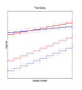
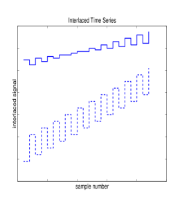
c)	d)

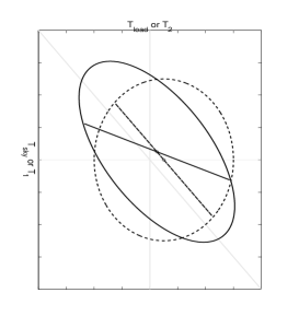
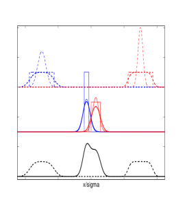
Figure 3: The effect of mixing and interlacing on time series (top frames) and distributions (low frames). in the output to the radiometer. Frame a) is an input time series, for sky (red dashed–line) and reference–load (blue dashed–line), and the corresponding mixed quantities $Q_{1}$ (red full–line), $Q_{2}$ (blu full–line) after mixing with $r_{1}=3/4$, $r_{2}=1/2$. The range of values allowed by noise within $\pm 5\sigma$ are represented in both mixed and not mixed quantities by the upper and lower dotted lines. The input time series has identical drifts on sky and reference–load equivalent to several noise $\sigma$s and corresponds to a signal dominated time serie as defined in Sect. 2.1. Frame b) are the signals as seen from the compressor after interlacing, full–line without mixing, dashed–line after mixing. Frame c) is the effect on a normal distribution and on a ramp, green before mixing and red after mixing. Frame d) shows the effect on the projected distributions after interlacing.

The effect of mixing with respect to both signals and distributions is illustrated in Fig. 3 which refers to the case of a data–stream which is signal dominated (see page 2.1). In this figure dashed–lines represent the input signals, full–lines the corresponding mixed signals, dotted–lines the limits for the variability induced by the noise. So the ramp in frame a) of Fig. 3 represents a model signal for ${T_{\mathrm{sky}}}(t)$ (blue dashed line) and ${T_{\mathrm{load}}}(t)$ (red dashed line). The corresponding interlaced data are shown in Fig. 3b (blue dashed–line), where the limits of variability induced by noise are not represented in order to avoid confusion. The time lines for $T_{1}(t)$ and $T_{2}(t)$ calculated for $r_{1}=3/4$, $r_{2}=1/2$, are represented in Fig. 3a and Fig. 3b as full–lines, and they are shifted to avoid overlapping with the previous plots. The reduction in the variance is associated with drifts in the mixed data is evident. Mixing transforms the bi–variate PDF which is for ${T_{\mathrm{sky}}}$, ${T_{\mathrm{load}}}$ signals into that for $T_{1}$, $T_{2}$. Fig. 3c represents its effect on the bi–variate PDF for the noise and the drift. Looking at the normal distributions of randomly variable signals in ${T_{\mathrm{sky}}}$ and ${T_{\mathrm{load}}}$, $g({T_{\mathrm{sky}}},{T_{\mathrm{load}}})$, the line for which $g({T_{\mathrm{sky}}},{T_{\mathrm{load}}})/g(\overline{T}_{\mathrm{sky}},\overline{T}_{\mathrm{load}})=1/2$ is a dashed line, and the equivalent line for $g(T_{1},T_{2})$ is a full-line. The distribution for the deterministic signal (either a ramp, a drift or a triangular wave) is represented by a segment, plotted again as a dashed line to denote the ${T_{\mathrm{sky}}}$, ${T_{\mathrm{load}}}$ signal and as a full line to denote the $T_{1}$, $T_{2}$. The effect of mixing is a combination of a non–uniform scaling, a rotation and a shift. The circle transforms into an ellipse. The line changes its tilt and length. In other terms, the covariance matrix for mixed data will be different from the original ones. A very interesting consequence is in the case of a normally distributed noise a correlated noise will appear in the mixed space even if the input noise is not correlated. In general after mixing the major axis of the two figures has the tendency to align with the $x=y$ line and the center of the two figures shifts. In this case $|\mathbf{M}|=r_{2}-r_{1}=1$ and the size of the two figures changes proportionally to $|\mathbf{M}|$. Interlacing transforms the bi–variate PDFs into univariate ones. Fig. 3d represents the effect of mixing on the PDF of interlaced data. Again, dashed lines represents the distributions before mixing and the full-lines after mixing. As in Fig. 3b red indicates ${T_{\mathrm{load}}}$ or $T_{1}$ and blue indicates ${T_{\mathrm{sky}}}$ or $T_{2}$. The bottom part of Fig. 3d represents the resulting distribution of interlaced signals, before (dashed) and after (full) the mixing.

How these distributions have to be decomposed in terms of the projected distributions is shown in the top part of Fig. 3d, which shows separately the distributions of the random and deterministic components, respectively a normal and a box distributions for ${T_{\mathrm{sky}}}$ and ${T_{\mathrm{load}}}$, The resulting distribution will be the convolution of the two, for ${T_{\mathrm{sky}}}$ and ${T_{\mathrm{load}}}$ are very similar to a box distribution. Of course the drift makes the overall signal non Gaussian, in particular for ${T_{\mathrm{load}}}$. The central part of Fig. 3d is the equivalent for the mixed signal. Here the drift is reduced and the convoluted signals are more similar to the original normal distributions of noises. I.e. mixing not only reduces the distance between the two components but, by reducing the drift, make them more normally distributed.

After mixing, the $(T_{1},T_{2})$ couples are re–quantized produce the quantized couples $(Q_{1},Q_{2})$ which are interlaced and sent to the compressor

$$Q_{i}=\mathrm{round}\left(\frac{T_{i}+\mathcal{O}}{q}\right),\;i=1,2;$$ (34)

where $\mathcal{O}$ is an offset introduced to force $(Q_{1},Q_{2})$ to stay within the range $[-2^{15},+2^{15}]$ . On ground, packets are entropy decoded, the data streams are de–interlaced and the corresponding $(Q_{1},Q_{2})$ are used to reconstruct the sky and reference–load samples

$$\tilde{T}_{\alpha}=\sum_{i=1,2}M^{-1}_{\alpha,i}[q\left(Q_{i}-\mathcal{O}\right)],\;\;\;\alpha=\mathrm{sky},\mathrm{load},$$ (36)

where $M^{-1}_{\alpha,i}$ are the components of $\mathbf{M}^{-1}$, and the tilde over a symbol “$\tilde{x}$” is used to distinguish a reconstructed quantity out of a processed one $x$.

Mixing will map sky—-reference–load statistics in the corresponding mixed statistics

$$\overline{T}_{i} = \overline{T}_{\mathrm{sky}}-r_{i}\overline{T}_{\mathrm{load}},\;i=1,2;$$ (37)

$$\Delta T_{\mathrm{i}} = \Delta T_{\mathrm{sky}}-r_{i}\Delta T_{\mathrm{load}},\;i=1,2;$$ (38)

$$\sigma_{i}^{2} = \sigma_{\mathrm{sky}}^{2}+r_{i}^{2}\sigma_{\mathrm{load}}^{2}-2r_{i}\sigma_{\mathrm{sky},\mathrm{load}};$$ (39)

$$\sigma_{1,2}^{2} = \sigma_{\mathrm{sky}}^{2}+r_{1}r_{2}\sigma_{\mathrm{load}}^{2}-\frac{r_{1}+r_{2}}{2}\sigma_{\mathrm{sky},\mathrm{load}}.$$ (40)

A simplification for the components of the covariance matrix can be obtained by assuming $\sigma_{\mathrm{sky}}$ as unitary, then defining $\breve{T}_{\alpha}=T_{\alpha}/\sigma_{\mathrm{sky}}$, $\alpha=$ $\mathrm{sky}$, $\mathrm{load}$; and incorporating $R_{\sigma}=\sigma_{\mathrm{sky}}/\sigma_{\mathrm{load}}$ in the $r_{i}$ factors. This gives these normalized parameters

$$\Delta\breve{T} = \breve{T}_{\mathrm{sky}}-r\breve{T}_{\mathrm{load}}$$ (41)

$$\breve{\sigma}_{i}^{2} = 1+\breve{r}_{i}^{2}-2\breve{r}_{i}\varrho_{\mathrm{s}\mathrm{l}};$$ (42)

$$\breve{\sigma}_{1,2}^{2} = 1+\breve{r}_{1}\breve{r}_{2}-\frac{\breve{r}_{1}+\breve{r}_{2}}{2}\varrho_{\mathrm{s}\mathrm{l}}.$$ (43)

where $\varrho_{\mathrm{s}\mathrm{l}}=\sigma_{\mathrm{sky},\mathrm{load}}/(\sigma_{\mathrm{sky}}\sigma_{\mathrm{load}})$, $\breve{r}_{i}=r_{i}/R_{\sigma}$. The corresponding transforms for the expectations is more complex. Of course $\overline{\breve{T}}_{\alpha}=\frac{\overline{T}_{\alpha}}{\sigma_{\mathrm{sky}}},\alpha=\mathrm{sky},\;\mathrm{load}$, but

$$\overline{{\breve{T}}}_{i} = \overline{\breve{T}}_{\mathrm{sky}}-R_{\sigma}\breve{r}_{i}\overline{\breve{T}}_{\mathrm{load}},\;i=1,2;$$ (44)

$$\Delta\breve{T}_{\mathrm{i}} = \Delta\breve{T}_{\mathrm{sky}}-R_{\sigma}\breve{r}_{i}\Delta\breve{T}_{\mathrm{load}},\;i=1,2.$$ (45)

However these normalizations are very useful in discussing the compression rate, especially after having defined the obvious $\breve{q}=q/\sigma_{\mathrm{sky}}$.

2.6 Modelling the statistical distribution of processed data

We want here to define an approximation able to asses $C_{\mathrm{r}}\geq C_{\mathrm{r}}^{\mathrm{Th}}$ in a simple way. For this reason we need to model the entropy for the signal entering the compressor. Of course the accuracy to which it is possible to predict the final $C_{\mathrm{r}}$ is directly connected to the accuracy to which the entropy is predicted. In the following we present two approximations for the entropy of the signal, a lower accuracy approximation and a high accuracy approximation.

2.6.1 The low accuracy approximation

Considering the usual reference cases of a noise dominated signal and a signal dominated by a linear drift, in the first case the PDF can be approximated by a normal distribution, in the second case the PDF can be approximated by a uniform distribution with $f_{Q}=q/A$ values and $\sigma=A/\sqrt{12}$. But in any case for $\sigma/q>>1$

$$H=\log_{2}k_{\mathrm{pdf}}\;\frac{\sigma}{q},$$ (47)

with $k_{\mathrm{pdf}}$ a constant depending on the type of p.d.f. ranging from $\sqrt{12}$ for a uniform distribution to $\sqrt{2\pi e}$ for a normal distribution. The difference in $H$ between these two extreme cases is $0.25$ bits. The argument of the logarithm is the number of symbols in the distribution. So $H$ may be written also as $H=\log_{2}N_{\mathrm{symb}}^{\mathrm{eff}}$ with $N_{\mathrm{symb}}^{\mathrm{eff}}=k_{\mathrm{pdf}}\sigma/q$. Of course in the case of the uniform distribution $N_{\mathrm{symb}}^{\mathrm{eff}}=N_{\mathrm{symb}}$. The PDF for the interlaced signals gives the probability to have a symbol $Q$ either from processes $Q_{1}$ or $Q_{2}$. Then

$$\mathcal{P}(Q)=\frac{\mathcal{P}_{1}(Q)+\mathcal{P}_{2}(Q)}{2}$$ (48)

with $\mathcal{P}_{i}(Q)$, $i=1$, 2 the marginal PDF for the $Q_{i}$ drawn from the bi–variate PDF $\mathcal{P}(Q_{1},Q_{2})$. For our extreme cases both $\mathcal{P}_{i}(Q)$ are uniformly distributed or normally distributed according to the original PDF from which they are drawn . This allows one to neglect, in estimating the entropy of the interlace signal, their mutual correlation. Then the entropy for the interlaced data is just a function of the RMS for the two distributions $\sigma_{1}$, $\sigma_{2}$, and their separation, $\breve{\Delta}_{\mathrm{distr}}$,

$$\breve{\Delta}_{\mathrm{distr}}=\frac{2}{k_{\mathrm{pdf}}}\frac{\mathrm{E}{\left[\breve{T}_{2}\right]}-\mathrm{E}{\left[\breve{T}_{1}\right]}}{\breve{\sigma}_{1}+\breve{\sigma}_{2}}$$ (49)

which is a normalized measure of the distance between the two peaks. After some algebra

$$\breve{\Delta}_{\mathrm{distr}}=2\frac{{\breve{r}_{1}-\breve{r}_{2}}}{k_{\mathrm{pdf}}}\frac{\overline{\breve{T}}_{\mathrm{load}}}{\breve{\sigma}_{1}+\breve{\sigma}_{2}}$$ (50)

Then the entropy will be just a function of $\breve{\sigma}_{1}$, $\breve{\sigma}_{2}$ and $\breve{\Delta}_{\mathrm{distr}}$. An exact analytical expression for $H$ can not be obtained for this case. However, it is easy to see that in the limit $|\breve{\Delta}_{\mathrm{distr}}|\gg 1$ the entropy takes the limiting value

$${H_{\infty}}=\frac{H_{1}+H_{2}}{2}+1,$$ (51)

giving

$${H_{\infty}}=\log_{2}(k_{\mathrm{pdf}})+\log_{2}(\sqrt{\breve{\sigma}_{1}\breve{\sigma}_{2}})-\log_{2}{\breve{q}}+1.$$ (52)

On the other side if $\breve{\Delta}_{\mathrm{distr}}=0$ and $\breve{\sigma}_{1}=\breve{\sigma}_{2}$ the two PDFs collapse giving $H_{0}=H_{1}=H_{2}$. In all the other cases $H_{0}\leq H(\Delta_{\mathrm{distr}})\leq{H_{\infty}}$. The important point here is the assumption that

$$H\approx{H_{\infty}},$$ (53)

would never overestimate the entropy by more than 1 bit or $\approx 30\%$. Therefore neglecting the compressor inefficiencies, a sufficient condition to asses $C_{\mathrm{r}}\geq C_{\mathrm{r}}^{\mathrm{Tgt}}$ would be

$${H_{\infty}}<H_{\mathrm{tgt}}$$ (54)

with $H_{\mathrm{tgt}}=N_{\mathrm{bits}}/C_{\mathrm{r}}^{\mathrm{Tgt}}$, or

$$\sqrt{\breve{\sigma}_{1}\breve{\sigma}_{2}}<\breve{q}\frac{2^{N_{\mathrm{bits}}/C_{\mathrm{r}}^{\mathrm{Tgt}}}}{2k_{\mathrm{pdf}}};$$ (55)

and so

$$\sqrt[4]{(1+\breve{r}_{1}^{2}-2\breve{r}_{1}\varrho_{\mathrm{s}\mathrm{l}})(1+\breve{r}_{2}^{2}-2\breve{r}_{2}\varrho_{\mathrm{s}\mathrm{l}})}<\breve{q}\frac{2^{N_{\mathrm{bits}}/C_{\mathrm{r}}^{\mathrm{Tgt}}}}{2k_{\mathrm{pdf}}};$$ (56)

Eq. (53), Eq. (54), Eq. (55) and Eq. (56) represent our low–order approximation for the optimization of REBA parameters. In particular, Eq. (56) puts a lower limit to $\breve{q}$ (and $q$) for a given $C_{\mathrm{r}}$. In fact for $\breve{r}_{1}=\breve{r}_{2}=0$, $\breve{q}$ must be larger or equal to

$$q_{\mathrm{min}}(C_{\mathrm{r}}^{\mathrm{Tgt}})=\frac{2k_{\mathrm{pdf}}}{2^{N_{\mathrm{bits}}/C_{\mathrm{r}}^{\mathrm{Tgt}}}}.$$ (57)

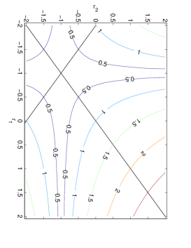
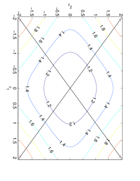
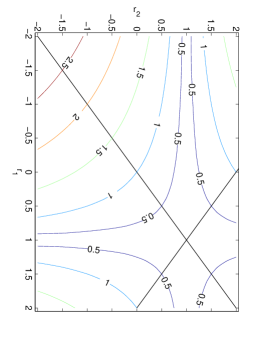
Figure 4: Iso–countour lines of the left side of Eq. (2.52) for $\varrho_{\mathrm{s}\mathrm{l}}=-1$ (left), $\varrho_{\mathrm{s}\mathrm{l}}=0$ (center) and $\varrho_{\mathrm{s}\mathrm{l}}=1$ (right). In the first case the function is minimal in the $(-1,-1)$ point, in the second in the $(0,0)$ point, while in the third in the $(1,1)$ point.

As shown in Fig. 4 for $\varrho_{\mathrm{s}\mathrm{l}}=0$, the left side of Eq. (56) in the $(\breve{r}_{1},\breve{r}_{2})$ plane has a minimum at $(0,0)$. Its iso–contour lines are closed, all centered on the origin, having four axis of symmetry $\breve{r}_{1}=0$, $\breve{r}_{2}=\pm\breve{r}_{1}$, and $\breve{r}_{2}=0$. The maximum distance from the origin of iso–contour lines occurs for $\breve{r}_{1}=0$ or $\breve{r}_{2}=0$ and the minimum occurs along the $\breve{r}_{2}=\pm\breve{r}_{1}$ line. Changing $\varrho_{\mathrm{s}\mathrm{l}}=0$ toward negative or positive values the iso–contour lines are again closed but their symmetry changes taking a more “cuspidal” shape, which is symmetrical about the $\breve{r}_{1}=\varrho_{\mathrm{s}\mathrm{l}}$ and the $\breve{r}_{2}=\varrho_{\mathrm{s}\mathrm{l}}$ lines. In any case, the value of the function decreases near the $\breve{r}_{2}=\breve{r}_{1}=\varrho_{\mathrm{s}\mathrm{l}}$ point where it has a minimum. From the figure it is evident that when converting $(\breve{r}_{1},\breve{r}_{2})$ to $(r_{1},r_{2})$ a larger $q/q_{\mathrm{min}}$ ratio or a smaller $\sigma_{\mathrm{load}}/\sigma_{\mathrm{sky}}$ increases the size of the region enclosed by each contour. Eq. (56) and Eq. (57) define in this low order approximation the optimal $q$ for which $C_{\mathrm{r}}=C_{\mathrm{r}}^{\mathrm{Tgt}}$

$$\breve{q}_{\mathrm{opt}}={q_{\mathrm{min}}(C_{\mathrm{r}}^{\mathrm{Tgt}})}{\sqrt[4]{(1+\breve{r}_{1}^{2}-2\breve{r}_{1}\varrho_{\mathrm{s}\mathrm{l}})(1+\breve{r}_{2}^{2}-2\breve{r}_{2}\varrho_{\mathrm{s}\mathrm{l}})}}$$ (58)

from which $q_{\mathrm{opt}}$ is simply derived as $q_{\mathrm{opt}}=\sigma_{\mathrm{sky}}\breve{q}_{\mathrm{opt}}$. This equation does not constrain completely $q_{\mathrm{opt}}$ and for this reason we have to take into account the processing error as explained in Sect. 2.7.

2.6.2 The high order accuracy approximation

The accuracy by which $q_{\mathrm{opt}}$ is determined by Eq. (58) is solely determined by the accuracy of imposing $H={H_{\infty}}$. Given the statistics of the input signal it would be not a problem to calculate by numerical integration $H$ as a function of $r_{1}$, $r_{2}$ and $q$. But of course this would be quite expensive from a computational point of view. For this reason a high accuracy algorithm to compute $H$ is derived Appendix A using simple equations from which $q_{\mathrm{opt}}$ could be readily obtained. However from the conceptual point of view the high accuracy method does not introduce any new detail in the discussion, and therefore the remaining part of this section refers only to the low–accuracy method unless otherwise stated.

2.7 Processing error of the mixing/demixing algorithm

The most important way to quantify the processing error is the measure of the distortion in the undifferentiated or differentiated data. The statistics of such distortions are taken as metrics of the quality of the process. For the undifferentiated data

$$\delta_{\alpha}=\tilde{T}_{\alpha}-T_{\alpha},$$ (59)

$\alpha=\mathrm{sky}$, $\mathrm{load}$. By following the methods of [Maris et al. (2004)] from Eq. (36) and Eq. (59) it is easy to derive the covariance matrix of the quantization error, $E_{q,\alpha,\beta}=\mathrm{cov}{\left[\delta_{\alpha},\delta_{\beta}\right]}$

$$\mathbf{E}_{\mathrm{q}}=\frac{q^{2}}{12}\frac{1}{(r_{2}-r_{1})^{2}}\left(\begin{array}[]{cc}r_{1}^{2}+r_{2}^{2},&r_{1}+r_{2}\\ r_{1}+r_{2},&2\\ \end{array}\right).$$ (60)

The distortion of differentiated data is instead expressed by

$$\delta_{\mathrm{diff}}=(\tilde{T}_{sky}-\tilde{r}\tilde{T}_{load})-({T_{\mathrm{sky}}}-r{T_{\mathrm{load}}});$$ (61)

where $\tilde{r}$ is the $r$ determined on the processed data, which in general will be slightly different from the $r$ determined on the original ones. However, assuming $\tilde{r}\approx r$ from Eq. (60) the variance of $\delta_{\mathrm{diff}}$ is

$$\epsilon_{q,\mathrm{diff}}^{2}=\frac{q^{2}}{12}\frac{(r_{2}-r)^{2}+(r_{1}-r)^{2}}{(r_{2}-r_{1})^{2}}$$ (62)

The first important fact which has to be stressed is that the variances of both errors are proportional to $q^{2}/(r_{2}-r_{1})^{2}$. Of course a nearly singular matrix with $r_{2}\approx r_{1}$ will result in very large errors. In addition, Eq. (60) shows that, despite quantization errors for $Q_{1}$ and $Q_{2}$ are uncorrelated, application of demixing causes processing errors in ${T_{\mathrm{sky}}}$ and ${T_{\mathrm{load}}}$ to be correlated unless

$$r_{1}+r_{2}=0.$$ (63)

However, expanding the numerator of Eq. (62) produces $\epsilon_{q,\mathrm{diff}}^{2}\propto r_{1}^{2}+r_{2}^{2}+2r^{2}-2r(r_{1}+r_{2})$ suggesting the important result that a not null correlation in the quantization errors may lead to a reduction of the error distortion in the differentiated data

Another very important case is $r_{1}=r$ or $r_{2}=r$. In this case Eq. (62) reduces to

$$\epsilon_{q,\mathrm{diff}}^{2}=\frac{q^{2}}{12}.$$ (64)

which is the same result we would have got quantizing differentiated data ([Maris et al. (2004), see]). This fact has been used in the first version of the optimization software, designed for the first run of the ground tests (the RAA tests described in [Bersanelli et al. (2009)]) to increase its speed, together with the fact that $C_{\mathrm{r}}$ and $\epsilon_{q}$ are not sensitive to an interchange of $r_{1}$ and $r_{2}$ but rather to $|r_{2}-r_{1}|$. However, in the subsequent tests the more general and accurate procedure described here has been successfully applied.

a)	b)
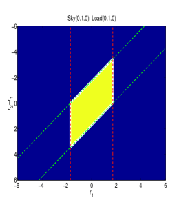
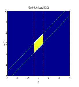
c)	d)

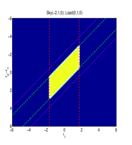
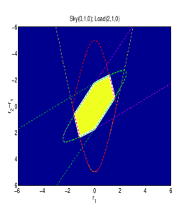
Figure 5: Example of analysis of $\mathcal{Q}_{\mathrm{ack}}$ factors in the $(r_{1},r_{2}-r_{1})$ space. Various cases for different values of ${T_{\mathrm{sky}}}$ and ${T_{\mathrm{load}}}$ are considered. The yellow region is the allowed region when all the $\mathcal{Q}_{\mathrm{ack},i}<1$, the blue region is the forbidden one. Thin dashed lines are the limits of allowed regions $\mathcal{Q}_{\mathrm{ack},1}$ with positive (red) or negative (yellow) drifts and $\mathcal{Q}_{\mathrm{ack},2}$ for positive (green) or negative (violet) drifts. Thin full lines are the allowed regions for $\mathcal{Q}_{\mathrm{ack},1}$ and $\mathcal{Q}_{\mathrm{ack},2}$ whose intersection is marked with a white thick line. Values of $\overline{T}_{\mathrm{sky}}$, $\sigma_{\mathrm{sky}}$, $\Delta T_{\mathrm{sky}}$ and the corresponding for ${T_{\mathrm{load}}}$ are between parentesis in the title of each frame in the order (mean, sigma, drift).

a)	b)
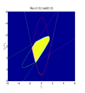
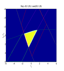
c)	d)

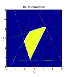
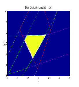
Figure 6: Example of analysis of $\mathcal{Q}_{\mathrm{ack}}$ factors. See caption of Fig. 5 for explanation of symbols.

2.8 Saturation

Saturation occurs when the argument of the $y=\mathrm{round}[x]$ function exceeds the maximum range of values allowed by the computer to represent the results. Indeed $y=\mathrm{round}[x]$ returns an $N_{\mathrm{bits}}$ signed integer. If $|x|>2^{N_{\mathrm{bits}}/2}$ an overflow or an underflow will occur. Depending on the implementation of the $y=\mathrm{round}[x]$ function the value of $y$ could be either forced to be $\pm 2^{15}$ with the sign depending on $x$, or modular arithmetic could be applied so that as an example a too large $x>0$ could be mapped into $y<0$. In all cases the whole subsequent reconstruction will produce meaningless results. So it is fundamental to avoid saturation.

The level of filling of the allowed dynamical range is measured by the instantaneous $\mathcal{Q}_{\mathrm{ack}}$ ratio

$$\mathcal{Q}_{\mathrm{ack},i}(t)=\frac{T_{i}(t)}{q2^{N_{\mathrm{bits}}-1}},i=1,2.$$ (65)

Saturation occurs if at some time $|\mathcal{Q}_{\mathrm{ack},i}(t)|\geq 1$ and the non–saturation condition is

$$|\mathcal{Q}_{\mathrm{ack},1}(t)|<1\wedge|\mathcal{Q}_{\mathrm{ack},2}(t)|<1;\;\forall t$$ (66)

in general this will put limits on $r_{1}$, $r_{2}$, $q$ and $\mathcal{O}$. Assuming to have applied the optimized offset of Eq. (78) the linear combinations are

$$\mathcal{Q}_{\mathrm{ack},1}(t) = \frac{{\Delta T_{\mathrm{sky}}}(t)-r_{1}\Delta T_{\mathrm{load}}(t)+\frac{r_{2}-r_{1}}{2}\overline{T}_{\mathrm{load}}\pm n\sigma_{n,1}}{q2^{N_{\mathrm{bits}}-1}}$$ (67)

$$\mathcal{Q}_{\mathrm{ack},2}(t) = \frac{{\Delta T_{\mathrm{sky}}}(t)-r_{2}\Delta T_{\mathrm{load}}(t)-\frac{r_{2}-r_{1}}{2}\overline{T}_{\mathrm{load}}\pm n\sigma_{n,2}}{q2^{N_{\mathrm{bits}}-1}}$$ (68)

where $n\approx 5$ is used to assess a safety region against random fluctuations.

In computing $\mathcal{Q}_{\mathrm{ack}}$ the effect of mutual cancellation of extremal values must be considered. A conservative estimate would be to propagate the modulus of each variation

$$\max(\Delta T_{i})=\max{|{\Delta T_{\mathrm{sky}}}|}+|r_{i}|\max{|\Delta T_{\mathrm{load}}|}+\left|\frac{r_{2}-r_{1}}{2}\right||\overline{T}_{\mathrm{load}}|+n\sigma_{i},$$ (69)

with $\min(\Delta T_{i})=-\max(\Delta T_{i})$, but it is better to explore the various combinations of minima and maxima within Eq. (67), producing a set of partial $\mathcal{Q}_{\mathrm{ack}}$ indexes which have to be independently satisfied. An example of such method is illustrated in Fig. 5 and Fig. 6.

In general, the separation between $T_{1}$ and $T_{2}$ is a function of time, whose measure is given by the divergence $\nabla T$, a parameter just sensitive to $\Delta T_{\mathrm{load}}$ and $\overline{T}_{\mathrm{load}}$

$$\nabla T(t)=-2\frac{(r_{2}-r_{1})(\Delta T_{\mathrm{load}}(t)+\overline{T}_{\mathrm{load}})}{k_{\mathrm{pdf}}(\sigma_{1}+\sigma_{2})}$$ (70)

of course $|\nabla T|$ will be constant when $\Delta T_{\mathrm{load}}=0$.

To determine the region of parameter space $r_{1}$, $r_{2}$ which satisfies Eq. (66) it is most convenient to work in the $(r_{1},r_{2}-r_{1})$ space, there the most general condition is

$$r_{1}(a-1)-b <r_{2}-r_{1}< r_{1}(a-1)-c;$$ (71)

$$c-(r_{2}-r_{1})(a-1) <(a-1)r_{1}< b-(r_{2}-r_{1})(a-1);$$ (72)

with the dimensionless coefficients

$$a = \left(\frac{2\Delta T_{\mathrm{load}}}{\overline{T}_{\mathrm{load}}}+1\right);$$ (73)

$$b_{\pm} = \frac{2}{\overline{T}_{\mathrm{load}}}\left({\Delta T_{\mathrm{sky}}}+q2^{N_{\mathrm{bits}}-1}\pm n\sigma\right);$$ (74)

$$c_{\pm} = \frac{2}{\overline{T}_{\mathrm{load}}}\left({\Delta T_{\mathrm{sky}}}-q2^{N_{\mathrm{bits}}-1}\pm n\sigma\right);$$ (75)

$$\sigma = \max(\sigma_{1},\sigma_{2});$$ (76)

For $n=0$ those conditions define a diamond–shaped region whose vertices are

$$\begin{array}[]{llll}A:&\left(\frac{c+b(a-1)}{a(a-1)},\frac{c-b}{a}\right),&B:&\left(\frac{b}{a-1},0\right),\\ &&&\\ C:&\left(\frac{b+c(a-1)}{a(a-1)},-\frac{c-b}{a}\right),&D:&\left(\frac{c}{a-1},0\right),\\ \end{array}$$

Note that $B:$ and $D:$ lie on $r_{2}-r_{1}=0$ line, while $A:$ and $D:$ are above and below it, the exact ordering depending on the signs. The center of the diamond–shaped region is locate on $((b+c)/(a-1),0)$. If $b+c=0$ the region is centered on the origin of the Cartesian system, $A:$, $C:$ and $B:$, $D:$ are mutually opposed. In the case $a=1$ the region degenerates into a band parallel to $r_{2}-r_{1}=0$, and bounded by $-b<r_{2}-r_{1}<-c$.

First considering the stationary case ${\Delta T_{\mathrm{sky}}}=0$, $\Delta T_{\mathrm{load}}=0$, then $a=1$, $b=-c$ the constraints for $n=0$. In this case $\mathcal{Q}_{\mathrm{ack},1}$ and $\mathcal{Q}_{\mathrm{ack},2}$ defines the same condition

$$|r_{2}-r_{1}|\frac{{T_{\mathrm{load},0}}}{2}<qN_{\mathrm{sat}}.$$ (77)

identifying simply a band around the $r_{1}=r_{2}$ line. The effect of noise is to put $n>0$ so that $a_{+}$ and $a_{-}$ are different and $\mathcal{Q}_{\mathrm{ack},1}$ defines a vertical band and $\mathcal{Q}_{\mathrm{ack},2}$ a diagonal band whose intersection is the diamond–shaped region above of Fig 5a. Changing the ratio between $\sigma_{n,2}/\sigma_{n,1}$ will not change the shape but just the size of the region, Fig 5b. Changing $\overline{T}_{\mathrm{sky}}$ and $\overline{T}_{\mathrm{load}}$ instead will change the shape of the allowed region as shown in Fig 5c, Fig 5d and Fig 6a. If $\overline{T}_{\mathrm{load}}=0$ the saturation condition becomes $|1-r_{i}|\cdot|A(t)|<qN_{\mathrm{sat}}$ i.e.: $1-qN_{\mathrm{sat}}/A_{\mathrm{max}}\leq r_{i}\leq 1+qN_{\mathrm{sat}}/A_{\mathrm{max}}$, with $A_{\mathrm{max}}=\max(|A(t)|)$. This defines a rectangular region with diagonal $r_{1}=r_{2}$. In the limiting case for $n=0$, $A_{\mathrm{max}}\rightarrow 0$ the allowed region becomes the whole plane, while in the opposite case $A_{\mathrm{max}}\rightarrow\infty$ the allowed region shrinks toward $r_{1}=r_{2}=1$.

Perturbations in the sky channel, such as the cosmological dipole, introduce a fluctuation which affects just the sky, in this case $\Delta T_{\mathrm{load}}=0$ and $a=1$. Even here the simplest cases are ${T_{\mathrm{load},0}}=0$, or the forbidden $r_{1}=r_{2}$. So $\max(|D(t)|)<qN_{\mathrm{sat}}$ is a sufficient condition which puts a limit just on $q$. In the most general case from Eq. (71) the limits of the allowed region are $-2{\Delta T_{\mathrm{sky}}}/{T_{\mathrm{load},0}}-2qN_{\mathrm{sat}}/{T_{\mathrm{load},0}}<r_{2}-r_{1}<-2{\Delta T_{\mathrm{sky}}}/{T_{\mathrm{load},0}}+2qN_{\mathrm{sat}}/{T_{\mathrm{load},0}}$

Other effects, such as instabilities of the 4–K reference–load, could affect just ${T_{\mathrm{load}}}$ and ${\Delta T_{\mathrm{sky}}}=0$, $b=2qN_{\mathrm{sat}}/{T_{\mathrm{load},0}}=-c$. Even here the simplest case $\overline{T}_{\mathrm{load}}=0$, $\max(|A(t)|)<qN_{\mathrm{sat}}$ is a sufficient condition which puts a limit just on $q$. In general a diamond–shaped region symmetrical around the origin represents the allowed region, as shown in Fig 6c.

Drifts in the gain of the amplifiers in the radiometers, such as those produced by thermal effects, add correlated or anticorrelated signals in sky and reference–load. So the model case to be considered is the one in which $A(t)\approx{\Delta T_{\mathrm{sky}}}(t)\approx\Delta T_{\mathrm{load}}(t)$. In this case with $a=(b+c)/2$ and Eq. (67) and Eq. (70) define the regions in Fig 6b and Fig 6d.

Before to conclude, it is interesting to consider the range of values assumed by $\mathcal{P}_{1}$ and $\mathcal{P}_{2}$ when $A$ in the range $A_{\mathrm{low}}<A<A_{\mathrm{up}}$ then $|P_{i,\mathrm{Up}}-P_{i,\mathrm{Low}}|=|A_{\mathrm{up}}-A_{\mathrm{low}}|\cdot|1-r_{i}|$. To have identical ranges, is $r_{1}\neq r_{2}$ and $r_{2}+r_{1}=2$ or $(r_{2}-r_{1})=2-2r_{1}$.

In nominal conditions, ${T_{\mathrm{sky},0}}\approx 2.73$ K, ${T_{\mathrm{load},0}}\approx 4$ K while ${T_{\mathrm{sky}}}$, ${T_{\mathrm{load}}}$ fluctuations are expected at the level of at most some $10^{-2}$ K giving $\Delta T_{\mathrm{load}}/{T_{\mathrm{load},0}}\approx{\Delta T_{\mathrm{sky}}}/{T_{\mathrm{load},0}}\approx\mathrm{some}\times 10^{-2}$, and hence $a\approx 1$, $b\approx-c$. But this condition could be severely violated at ground during the ground tests, or in flight while the instrument is cooling down.

3 Optimizing the On–board Processing

The optimization of the algorithm consists in determining the “best” combination of the set of processing parameters i.e. the “best” n–tuple $N_{\mathrm{aver}}$, $r_{1}$, $r_{2}$, $\mathcal{O}$, $S_{\mathrm{q}}$ or $q$. It is mandatory that the optimization procedure will keep within safe limits $C_{\mathrm{r}}=C_{\mathrm{r}}^{\mathrm{Tgt}}$.

The classical approach would require a function of merit and a searching algorithm through the corresponding $N\times R^{4}$ parameters space to be applied to each of the 44 detectors. However a reduction of the cardinality of space comes from the fact that, by-requirement, the nominal $N_{\mathrm{aver}}$ is fixed by the oversampling factor for the beam, so apart from the cases in which a different oversampling is required, the $N_{\mathrm{aver}}$ in nominal conditions is fixed. The only cases in which $N_{\mathrm{aver}}$ could be varied are: i.) sampling of planets for beam reconstruction; ii.) ground testing and diagnostics. The first case occurs when the beam has to be reconstructed with higher detail than the one reachable with the nominal oversampling factor $n_{\mathrm{over}}=3$. So it is possible to ask the on–board processor to decrease $N_{\mathrm{aver}}$ increasing proportionally the data–rate from the feed–horns which will be affected by a planet. To arrange the higher–throughput of scientific telemetry, $q$ will have to be increased, increasing proportionally $\epsilon_{q}$. In the second case the value of $N_{\mathrm{aver}}$ could be varied either to increase the time resolution, as an example if sampling of some perturbation characterized by time scales compatible to $N_{\mathrm{aver}}/f_{\mathrm{sampling}}$ has to be investigated, or if some temporary shortage in the telemetry rate is imposed, asking in this case to increase $N_{\mathrm{aver}}$. Also while testing on ground for long term drifts, the sky is replaced by a dummy load at constant temperature. In this case time resolution is no longer an asset and $N_{\mathrm{aver}}$ could be increased. A further reduction of the parameter space to be explored comes from the fact that usually $\mathcal{O}$ is optimized in order to have $\mathrm{mean}{\left[T_{\mathrm{interlaced}}+\mathcal{O}\right]}=0$ where $T_{\mathrm{interlaced}}$ are the interlaced samples produced after by Eq. (29). It is then easy to derive that $\mathrm{mean}{\left[T_{\mathrm{interlaced}}+\mathcal{O}\right]}=\mathrm{mean}{\left[T_{1}\right]}+\mathrm{mean}{\left[T_{2}\right]}+2\mathcal{O}$ so that $\mathcal{O}_{\mathrm{optimal}}=-(\mathrm{mean}{\left[T_{1}\right]}+\mathrm{mean}{\left[T_{2}\right]})/{2}$, and with some simple algebra

$$\mathcal{O}_{\mathrm{optimal}}=-\overline{T}_{\mathrm{sky}}+\frac{r_{1}+r_{2}}{2}\overline{T}_{\mathrm{load}},$$ (78)

where the mean has to be computed over a suitable time span. What remains is a $\Re^{3}$ parameter space to be explored $(r_{1},r_{2},q)$.

3.1 Target function

The target function $\chi(r_{1},r_{2},q)$ for the optimization would i.) asses $C_{\mathrm{r}}=C_{\mathrm{r}}^{\mathrm{Tgt}}$ to be kept within safe limits; ii.) asses $\epsilon_{q}$ to be kept as small as possible; iii.) asses additive constrains. These constrains do not allow a unambiguous definition of a target function. As an example, even for a stationary signal dominated by white noise, $C_{\mathrm{r}}$ computed on each packet is a random variable. So the question is whether $C_{\mathrm{r}}=C_{\mathrm{r}}^{\mathrm{Tgt}}$ has to be interpreted strictly, i.e. forcing each packet to have $C_{\mathrm{r}}=C_{\mathrm{r}}^{\mathrm{Tgt}}$ or on average leaving space for lower and higher $C_{\mathrm{r}}$? In general it would not be critical if some fraction of the packets would be compressed at a rate lower than $C_{\mathrm{r}}^{\mathrm{Tgt}}$. The requirement on $\epsilon_{q}$ is even worse defined. Of which $\epsilon_{q}$ are we speaking? As shown in sect. 2.5 it is evident that there is not a general definition for $\epsilon_{q}$. Depending on the scope of the data acquisition it could be more interesting to have a low $\epsilon_{q}$ for ${T_{\mathrm{sky}}}$ or ${T_{\mathrm{load}}}$ or $\Delta T$ computed for some reference $r$. More over neither $\epsilon_{q}$ nor $\epsilon_{q,\mathrm{diff}}$ are functions with a minimum and they vary over the full range of positive values. In addition within a pointing period $N$ repeated sky samples are acquired. In making maps repeated samples are averaged and $\epsilon_{q}$ will be reduced by a factor $1/\sqrt{N}$ [Maris et al. (2004)]. So a relatively high $\epsilon_{q}$ could be acceptable at the level of single samples when observing stationary sources. However the ratio between $\epsilon_{q}$ and the noise will not change after averaging. So a convenient choice would be to consider $\epsilon_{q}/\sigma$, where $\sigma$ could be the RMS of ${T_{\mathrm{sky}}}$, ${T_{\mathrm{load}}}$ or $\Delta T$ depending on the case. The only hard constraint which has to be considered is that saturation must be avoided.

The general formula for the target function is

$$\chi(\mathbf{\Theta})=\prod_{c}{\mathcal{Q}_{c}(\mathbf{\Theta})}^{\Pi_{c}},$$ (79)

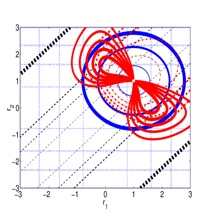
Figure 7: Iso contour lines for the functions entering $\epsilon_{q,\mathrm{diff}}$ and $\epsilon_{q,\mathrm{diff}}$ as a function of ($r_{1}$, $r_{2}$). Vertical blue dashed lines $\sigma_{1}$, horizontal blue dashed lines $\sigma_{2}$, black dashed lines $(r_{2}-r_{1})^{2}$, blue contours $(r_{1}-r)^{2}+(r_{2}-r)^{2}$, red dashed contours $\sqrt{\sigma_{1}\sigma_{2}}$, and the red contours are the resulting $\epsilon_{q,\mathrm{diff}}$. The width of the lines varies with the value of the function.

$\mathbf{\Theta}$ is a vector in the parameter space, $\mathcal{Q}_{c}$ is a function varying over the range $[0,1]$ with $\mathcal{Q}_{c}(\Theta)=1$ if $\Theta$ fits the particular criterion $c$ for which the function is defined, $\mathcal{Q}_{c}(\Theta)=0$ if $\Theta$ does not fit this criterion. Intermediate values may be also defined in the [0,1] range measuring the goodness of fit. As an example, a criterion for optimal $q$ is to have $\gamma_{\mathrm{diff}}=\min(\gamma_{\mathrm{diff}})$, the corresponding criterion function is $\mathcal{Q}_{c}(\Theta)=\min(\gamma_{\mathrm{diff}})/\gamma_{\mathrm{diff}}$. The exponents $\Pi_{c}\geq 0$, with $\sum_{c}\Pi_{c}=1$, are weights defining the relative importance of each criterion within a given policy. In general it is better to have $\mathcal{Q}_{c}(\Theta)$ functions which are derivable. In some case it is necessary to to deal with poles that have to be avoided. A method is to define a metric $\mu_{c}(\Theta)\geq 0$ with a single pole for which $\mu_{c}(\Theta)\rightarrow+\infty$ and take $\mathcal{Q}_{c}(\Theta)=e^{-\mu_{c}(\Theta)}$ or $\mathcal{Q}_{c}(\Theta)=1/(1+e^{-\mu_{c}(\Theta)})$. Typical criteria are shown in Tab. 1

Table 1: List of possible criteria

Condition	Criterium
$\epsilon_{q,\mathrm{diff}}=\min(\epsilon_{q,\mathrm{diff}})$	$\mathcal{Q}_{c}=\min(\epsilon_{q,\mathrm{diff}})/\epsilon_{q,\mathrm{diff}}$
$\epsilon_{q,\mathrm{sky}}=\min(\epsilon_{q,\mathrm{sky}})$	$\mathcal{Q}_{c}=\min(\epsilon_{q,\mathrm{sky}})/\epsilon_{q,\mathrm{sky}}$
$\epsilon_{q,\mathrm{load}}=\min(\epsilon_{q,\mathrm{load}})$	$\mathcal{Q}_{c}=\min(\epsilon_{q,\mathrm{load}})/\epsilon_{q,\mathrm{load}}$
$\epsilon_{q,\mathrm{load}}=\epsilon_{q,\mathrm{diff}}$	$\mathcal{Q}_{c}=1-|\epsilon_{q,\mathrm{load}}-\epsilon_{q,\mathrm{diff}}|/\max(\epsilon_{q,\mathrm{load}}+\epsilon_{q,\mathrm{sky}})$
$\epsilon_{q,\mathrm{load}}=\epsilon_{q,\mathrm{sky}}$	$\mathcal{Q}_{c}=1-|\epsilon_{q,\mathrm{load}}-\epsilon_{q,\mathrm{sky}}|/\max(\epsilon_{q,\mathrm{load}}+\epsilon_{q,\mathrm{sky}})$
$\epsilon_{q,\mathrm{diff}}=\epsilon_{q,\mathrm{sky}}$	$\mathcal{Q}_{c}=1-|\epsilon_{q,\mathrm{diff}}-\epsilon_{q,\mathrm{sky}}|/\max(\epsilon_{q,\mathrm{diff}}+\epsilon_{q,\mathrm{sky}})$

a)	b)
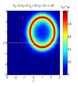
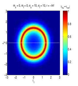
c)	d)

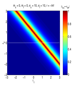
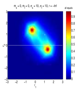
Figure 8: Comparison for $\epsilon_{q,\mathrm{diff}}=\epsilon_{q,\mathrm{sky}}$ top–left, $\epsilon_{q,\mathrm{diff}}=\epsilon_{q,\mathrm{load}}$ top– right, $\epsilon_{q,\mathrm{sky}}=\epsilon_{q,\mathrm{load}}$ bottom–left and the corresponding best fit regions bottom–right; as a function of ($r_{1}$, $r_{2}$). The lines are iso–contours of $\exp(-|x|)$ where $x$ is the difference between the two arguments to be compared. For the bottom–right frame the iso–contours are tracked for cubic root of the product of the comparison functions. The simulation is for $\overline{T}_{\mathrm{sky}}=\overline{T}_{\mathrm{load}}=0$, $\sigma_{\mathrm{sky}}=\sigma_{\mathrm{load}}=10$ ADU, $r=1$. No drifts are included.

a)	b)
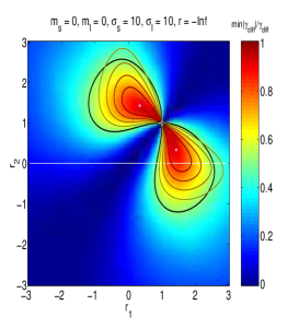
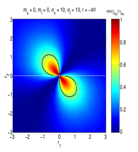
c)	d)

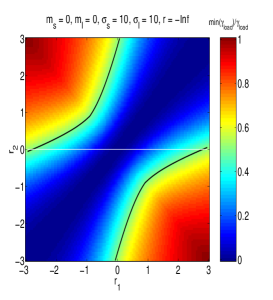
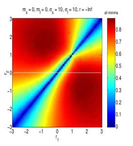
Figure 9: Iso contour lines identifiing the regions in the ($r_{1}$, $r_{2}$) space where $\min(\epsilon_{q,\mathrm{diff}})/\epsilon_{q,\mathrm{diff}}$ top–left, $\min(\epsilon_{q,\mathrm{sky}})/\epsilon_{q,\mathrm{sky}}$ top–right, $\min(\epsilon_{q,\mathrm{load}})/\epsilon_{q,\mathrm{load}}$ bottom–left, and where all of the $\epsilon_{q}$ are as near as possible at their minima, bottom–right. The lines are isocontours of $\min(x)/x$ which is 1 when the minimum is reached. For the bottom–right frame the iso–contours are the cubic root of the product of the other frames. In the top–left frame white $+$ denotes the positions of the analytical solution, the black thick contour is for $\min(\epsilon_{q,\mathrm{diff}})/\epsilon_{q,\mathrm{diff}}=0.5$, the black thin contour lines are for $\min(\epsilon_{q,\mathrm{diff}})/\epsilon_{q,\mathrm{diff}}$ assuming $H\equiv{H_{\infty}}$. The simulation is for $\overline{T}_{\mathrm{sky}}=\overline{T}_{\mathrm{load}}=0$, $\sigma_{\mathrm{sky}}=\sigma_{\mathrm{load}}=10$ ADU, $r=1$. No drifts are included.

3.2 Analytical Optimization

Analytical optimization (AO) is based on analytical formulas assuming either normally distributed or uniformly distributed signals. As a starting point for more refined numerical optimization. At the root of this method of optimization is the requirement of minimizing the processing errors, as an example the $\epsilon_{q,\mathrm{diff}}$. However given they diverge at $r_{1}=r_{2}$ it is necessary to consider the maximization of their inverse normalized to the minimal value, as an example defining for $\epsilon_{q,\mathrm{diff}}$ the function $\Gamma_{\mathrm{diff}}=\min(\epsilon_{q,\mathrm{diff}})/\epsilon_{q,\mathrm{diff}}$. These functions become 0 for $\breve{r}_{1}=\breve{r}_{2}$, unless either $\breve{r}_{1}=\breve{r}$ or $\breve{r}_{2}=\breve{r}$.

Again it is convenient to use the normalized parameters $\breve{r}_{i}$, in this case the covariance matrix of the processing errors is

$$\mathbf{\breve{E}}_{\mathrm{q}}=\frac{\breve{q}^{2}}{12}\frac{1}{(\breve{r}_{2}-\breve{r}_{1})^{2}}\left(\begin{array}[]{cc}\breve{r}_{1}^{2}+\breve{r}_{2}^{2},&\frac{\breve{r}_{1}+\breve{r}_{2}}{R_{\sigma}}\\ \frac{\breve{r}_{1}+\breve{r}_{2}}{R_{\sigma}},&\frac{2}{R_{\sigma}^{2}}\\ \end{array}\right).$$ (80)

In the framework of the low–level approximation for $q_{\mathrm{opt}}$ calculation, after replacing Eq. (58) into the $\epsilon_{q,\mathrm{diff}}$ from Eq. (62), substituting $r_{i}\rightarrow\breve{r}_{i}$, $q\rightarrow\breve{q}$ and $r\rightarrow\breve{r}=r/R_{\sigma}$, its reciprocal is

$$\Gamma_{\mathrm{diff}}=\frac{(\breve{r}_{2}-\breve{r}_{1})^{2}}{\left[(\breve{r}_{1}-\breve{r})^{2}+(\breve{r}_{2}-\breve{r})^{2}\right]\sqrt[4]{(1+\breve{r}_{1}^{2}-2\breve{r}_{1}\varrho_{\mathrm{s}\mathrm{l}})(1+\breve{r}_{2}^{2}-2\breve{r}_{2}\varrho_{\mathrm{s}\mathrm{l}})}}$$ (81)

$\Gamma_{\mathrm{diff}}$ is symmetrical with respect to the axis $\breve{r}_{1}=\breve{r}_{2}$ and has a maximum where the processing error has a minimum. There is no analytical way to maximize $\Gamma_{\mathrm{diff}}$. However, Fig. (7) shows the contour plot for the various components of this function. The denominator is the product of a function which is constant over circles centered on $\breve{r}_{1}=\breve{r}_{2}=\breve{r}$ (or $r_{1}=r_{2}=r$) and which increases with the radius, and of $\sqrt{\breve{\sigma}_{1}\breve{\sigma}_{2}}$ which has a more or less elliptical form and that for $\varrho_{\mathrm{s}\mathrm{l}}=0$ is centered on $\breve{r}_{1}=\breve{r}_{2}=0$. The numerator is null on the $\breve{r}_{1}=\breve{r}_{2}$ line and it is constant over lines parallel to $\breve{r}_{1}=\breve{r}_{2}$ increasing with distance from that line. Hence the $\Gamma_{\mathrm{diff}}$ maxima must be symmetrically aligned along a line normal to $\breve{r}_{1}=\breve{r}_{2}$. The line has to cross the $\breve{r}_{1}=\breve{r}_{2}$ line at $\breve{r}_{1}=\breve{r}_{2}=\breve{r}_{\mathrm{c}}$, with $0\leq\breve{r}_{\mathrm{c}}\leq\breve{r}$, so that the maxima for $\Gamma_{\mathrm{diff}}$ are located at

$$\breve{r}_{1} \simeq \breve{r}_{\mathrm{c}}\pm\frac{1}{\sqrt{2}}\breve{\ell}_{\mathrm{min}},$$ (82)

$$\breve{r}_{2} \simeq \breve{r}_{\mathrm{c}}\mp\frac{1}{\sqrt{2}}\breve{\ell}_{\mathrm{min}};$$ (83)

where $\breve{\ell}_{\mathrm{min}}$ measures their distance from the $\breve{r}_{1}=\breve{r}_{2}$ line. Numerically it is possible to show that in the case $\varrho_{\mathrm{s}\mathrm{l}}=0$ sufficient numerical approximations to $\breve{\ell}_{\mathrm{min}}$ and $\breve{r}_{\mathrm{c}}$ as a functions of $\breve{r}$ are,

$$\breve{r}_{\mathrm{c}} \approx 0.6994\breve{r}+0.2722$$ (84)

$$\breve{\ell}_{\mathrm{min}} \approx \left\{\begin{array}[]{ll}&\\ 0,&0<\breve{r}\leq 0.701\\ -3.0836\breve{r}^{2}+6.7034\breve{r}+3.0969,&0.701<\breve{r}<1\\ -0.3985\breve{r}^{2}+0.3367\breve{r}-0.4369,&1\leq\breve{r}\leq 10\\ &\\ \end{array}\right.$$ (90)

Fig. 9a represents a typical pattern for $\Gamma_{\mathrm{diff}}(r_{1},r_{2})$ (the $\breve{r}_{i}$ are converted into $r_{i}$), and it is assumed $r=1/R_{\sigma}$. The optimization produced by maximizing Eq. (81) could be improved by using the approximation for the entropy in Sect. A which takes into account of possible overlaps between the $Q_{1}$ and $Q_{2}$ distributions, allowing a better approximation to $q_{\mathrm{opt}}(r_{1},r_{2})$. So in the figure $\Gamma_{\mathrm{diff}}$ have been computed by using the method in Appendix A but black contour lines are those obtained assuming $H={H_{\infty}}$ at the root of Eq. (81) it is evident that the two approximations agree quite well. Crosses mark the position of maxima calculated with the approximated solution described above. The $\mathcal{Q}_{\mathrm{ack}}$ factor for this case does not reveal any saturation. So it is possbile to look for other combinations of optimized parameters. As an example: Fig. 9 b) and c) are the equivalent of $\Gamma_{\mathrm{diff}}$ computed for $\epsilon_{q,\mathrm{sky}}$, and $\epsilon_{q,\mathrm{load}}$. Of course while $\Gamma_{\mathrm{sky}}$ has well defined maxima this is not true for $\Gamma_{\mathrm{load}}$ given $\epsilon_{q,\mathrm{load}}$ has not an upper limit. Fig. 9 d) represents the product of $\Gamma_{\mathrm{diff}}$ and $\Gamma_{\mathrm{sky}}$. We may look at combinations of parameters where, $\epsilon_{q,\mathrm{sky}}=\epsilon_{q,\mathrm{load}}$ or $\epsilon_{q,\mathrm{sky}}=\epsilon_{q,\mathrm{diff}}$ or $\epsilon_{q,\mathrm{load}}=\epsilon_{q,\mathrm{sky}}$ as in Fig. 8a,b and c, or $\epsilon_{q,\mathrm{diff}}\approx\epsilon_{q,\mathrm{load}}\approx\epsilon_{q,\mathrm{sky}}$. Thus the product of the second group of criteria in Tab. 1 can be used, assuming all the $\Pi_{c}=1/4$, as shown in Fig. 8d.

3.3 Dealing with saturation

A more complex situation could arise if the selected optimal $r_{1}$, $r_{2}$ and $q_{\mathrm{opt}}$ lead to saturation. In this case either a $(r_{1},r_{2},q_{\mathrm{opt}})$ far from the $\Gamma_{\mathrm{diff}}$ peak has to be selected or $q_{\mathrm{opt}}$ has to be increased in order to reduce the corresponding $\mathcal{Q}_{\mathrm{ack}}$ factor. In the first case the requirement $C_{\mathrm{r}}=C_{\mathrm{r}}^{\mathrm{Tgt}}$ will be assessed but the quantization error will be larger than the optimal one. To limit this error the new $(r_{1},r_{2},q_{\mathrm{opt}})$ would have to be selected as much as possible along the ridge near the $\Gamma_{\mathrm{diff}}$ peak ad as much as possible far from the $r_{1}=r_{2}$ line. In the second case we consider the fact that $\mathcal{Q}_{\mathrm{ack}}\propto 1/q$ so it is possible to take $r_{1}$ and $r_{2}$ at the $\Gamma_{\mathrm{diff}}$ peak but to take

$$q_{\mathrm{opt},\mathcal{Q}{\mathrm{ack}}}=\mathcal{S}_{\mathrm{ft}}\mathcal{Q}_{\mathrm{ack},1}^{\mathrm{max}}q_{\mathrm{opt}}(r_{1}^{\mathrm{peak}},r_{2}^{\mathrm{peak}})$$

where $\mathcal{Q}_{\mathrm{ack},1}^{\mathrm{max}}=\max(|\mathcal{Q}_{\mathrm{ack},1}^{\mathrm{peak}}|,|\mathcal{Q}_{\mathrm{ack},2}^{\mathrm{peak}}|)$ and $\mathcal{S}_{\mathrm{ft}}>1$ is a safety factor which typically is $\mathcal{S}_{\mathrm{ft}}=2$. Of course in this case the data are compressed at an higher rate than $C_{\mathrm{r}}^{\mathrm{Tgt}}$ while the processing error will be increased by a factor $\mathcal{S}_{\mathrm{ft}}\mathcal{Q}_{\mathrm{ack},1}^{\mathrm{max}}$.

3.4 OCA2K, non idealities and numerical optimization

Non–idealities in the signal and in the compressor cause the effective $C_{\mathrm{r}}$ to be different from the expected $C_{\mathrm{r}}^{\mathrm{Th}}$, and in general $C_{\mathrm{r}}^{\mathrm{Th}}>C_{\mathrm{r}}$. A formal way to account for this is to define a compression efficiency $\eta_{C_{\mathrm{r}}}\leq 1$ defined as:

$$\eta_{C_{\mathrm{r}}}=\frac{C_{\mathrm{r}}}{C_{\mathrm{r}}^{\mathrm{Th}}},$$ (91)

which could be decomposend in the product of the contributions of each non–ideality. In general it is very difficult to account in a satisfactory way for even the most important non idealities as is illustrated by the following examples.

A group of non–idealities comes from the fact that each time a new symbol is discovered in the data stream the compressor adds at the compressed output a “stop” pseudo–symbol followed by the uncompressed symbol. Then the compressor is coding the symbols in the input data stream plus the “stop” pseudo–symbol and consequently the entropy for the compressed data stream to be introduced into Eq. (17) is changed by a factor $\eta_{\mathrm{stop}}^{-1}$

$$\eta_{\mathrm{stop}}^{-1}=-\frac{\varphi_{\mathrm{stop}}}{1+\varphi_{\mathrm{stop}}}\log_{2}\frac{\varphi_{\mathrm{stop}}}{1+\varphi_{\mathrm{stop}}}+\frac{1+\log_{2}(1+\varphi_{\mathrm{stop}})}{H(1+\varphi_{\mathrm{stop}})},$$ (92)

where $\varphi_{\mathrm{stop}}=N_{\mathrm{symb}}/n_{\mathrm{samples}}$, $N_{\mathrm{symb}}$ is the number of different symbols in the packet, $n_{\mathrm{samples}}$ the number of samples stored in the packet and $H$ comes from Eq. (17). Note that for $\varphi_{\mathrm{stop}}\rightarrow 0$, $\eta_{\mathrm{stop}}^{-1}\rightarrow 1$. In general for small $\varphi_{\mathrm{stop}}$ the addition of stopping symbols increases the entropy leading to $\eta_{\mathrm{stop}}<1$, but when $\varphi_{\mathrm{stop}}$ is sufficiently large the compressed data chunk is diluted in a large number of repeated symbols, reducing the entropy of the signals and giving $\eta_{\mathrm{stop}}>1$. However the potential gain in $C_{\mathrm{r}}^{\mathrm{Th}}$ is compensated by the need to add uncompressed symbols. If $N_{\mathrm{bits},\mathrm{code}}$ is the number of bits needed to store the information used to decode a symbol, ${L_{\mathrm{pck}}}$ is the length of the packet, then from the condition

$$\frac{n_{\mathrm{samples}}N_{\mathrm{bits}}}{C_{\mathrm{r}}^{\mathrm{Th}}}+N_{\mathrm{symb}}N_{\mathrm{bits},\mathrm{code}}\leq{L_{\mathrm{pck}}};$$

and from $L_{\mathrm{in}}=n_{\mathrm{samples}}N_{\mathrm{bits}}$, assuming the optimal case $L_{\mathrm{out}}={L_{\mathrm{pck}}}$ the dumping factor for the compression efficiency is derived

$$\eta_{\mathrm{store}}=\left[1+\frac{N_{\mathrm{symb}}}{n_{\mathrm{samples}}}\frac{N_{\mathrm{bits},\mathrm{code}}}{N_{\mathrm{bits}}}C_{\mathrm{r}}^{\mathrm{Th}}\right]^{-1}.$$ (93)

In general, for a stationary signal $N_{\mathrm{symb}}\ll n_{\mathrm{samples}}$ so that $\eta_{\mathrm{store}}$ is a second order correction which will be neglected in the remaining of the text, but it becomes important in the case of non–stationary signals for which $N_{\mathrm{symb}}\approx n_{\mathrm{samples}}$, which could occur in case of fast drifts.

Two non–idealities very complicated to be analyzed are the difference between the expected entropy and the sampling entropy, and the compressor inertia.

The theoretical estimates of entropy and hence of the expected compression rate, gives the expected entropy calculated on an ideally infinite number of realizations of samples. This means that even very infrequent symbols for the samples are considered by theory. But the compressor stores a few hundreds of samples for each packet leading to a truncated distribution of samples and consequently to a sampled entropy which in general is smaller than both the theoretical expectation and the entropy measured on a long data stream. In theory if $G(Q)$ is the cumulative PDF for the distribution of samples, and if $Q$ is bounded between $Q_{\mathrm{inf}}$ and $Q_{\mathrm{sup}}$ it would be sufficient to rescale the $f_{Q}$ by $1/(G(Q_{\mathrm{sup}})-G(Q_{\mathrm{inf}}))$ and redefine accordingly the sum in the definition of the Shannon entropy. As an example, in the case of a simple normal distribution cutting the distribution respectively at $1$, 2, 3 and $4\sigma$ will reduce the entropy as predicted from Eq. (47) respectively by a factor $\eta_{C_{\mathrm{r}}}=0.79$, 0.89, 0.95 and 0.98. However, the difference between theoretical entropy, or even the entropy measured on long data streams, and the sampling entropy measured on short packets could be changed by the presence of correlations in the signals on scales longer than the typical time scale of a packet. Last but not least, it is necessary to consider that the compressor takes some time to optimize its coding scheme, leading to a further loss in compression efficiency.

The effect of all of these non idealities are too complicated to be introduced in the theoretical model, so that the tuning of REBA parameters based on the theoretical models has to be refined by numerical optimisation. Numerical optimisation it is important to handle difficult cases in which the hypothesis of the theoretical model fails, it allows experimentation with artificial perturbations introduced in the signal and it includes higher order effects such as the packet–by–packet variability of $C_{\mathrm{r}}$, In addition numerical simulations must be used to verify the optimized parameters before uploading them to the instrument.

With these aims the Onboard Computing Analysis (OCA) software was developed, composed of a scanner, able to run the same test on different combinations of REBA parameters; an analyzer, able to automatically extract relevant statistics on each test; an optimizer, able to apply different policies defining when a combination of parameters is optimal or not selecting the best combinations; a report generator, used to generate automated reports. Apart from REBA optimization the development of the OCA libraries has been driven by the need to have a flexible environment for testing ground segment operations as explained in [Fraillis et al. (2008b)]. Hence, OCA is able to read, decode, and process small amounts of raw data coming from the Planck/LFI scientific pipeline from packets to complete timelines.

At the core of the part of the OCA software dedicated to the REBA optimization there is a C++ kernel, (OCA2K) which processes the input data for each combination of REBA parameters performing: i. on–board mixing and quantization by using the real algorithm; ii. on–board compression by using the on–board algorithm; iii. on ground decompression and reconstruction.

It has to be noted that OCA2K uses the same C code for compression operated on–board. So it does not emulate the compressor but uses the real compressor. In addition the validation of proper emulation of the on–board and on–ground processing has been provided by using data generated in the framework of the validation of Level–1. of the Planck/LFI DPC [Fraillis et al. (2008b)]. In that way we demonstrated that OCA2K processes the data in the same manner as the real processing chain.

The input of OCA and OCA2K are short data streams of raw data downloaded from the instrument just before on–board averaging or just after it (see Fig. 2) depending on whether $N_{\mathrm{aver}}$ has to be optimized or not. In output OCA2K provides packet–by–packet measures of $C_{\mathrm{r}}$ and its related quantities such as the estimated packet entropy, or the measured compression efficiency $\eta_{\mathrm{oca2k}}$. It provides also sample–by–sample estimates of critical parameters as $\epsilon_{q}$, and $\mathcal{Q}_{\mathrm{ack}}$.

Despite OCA2K is written in C++, it remains a heavy, offline tool, which can not be directly used for a crude exhaustive real–time optimization. This is the reason for which analytical methods have been developed. On the contrary OCA has the ability to use the analytical models to focus on the relevant region of parameters space.

OCA allows the determination of the optimum parameters according to different optimization strategies and constraints. This is important given the different ways in which REBA parameters are optimized during ground tests and in flight. During ground testing the usual procedure has been to stabilize the instrument and its environment, calibrate the DAE and then to acquire chunks of about 15 minutes of averaged data to be analyzed by OCA to optimize the REBA parameters [Cuttaia at al.(2009)]. After setting the REBA parameters another session of 15 minutes of acquisition, this time with the nominal processing described in Fig. 2 is executed as a cross-check. In flight the procedure will be to acquire continuously data by using the nominal processing Short chunks of unprocessed data will be acquired daily in turn from each detector. The comparison of unprocessed with processed data will allow to monitor of the processing error. In addition the REBA tuning might be repeated daily on the chunck of unprocessed data in order to test whether some REBA parameters on–board the satellite should be changed or not.

OCA could be used as a stand–alone application, but different interfaces for OCA to other packages have been created for different applications. For ground segment testing OCA provided an IDL and C++ library used in a stand–alone program. The same occurred for the Planck/LFI simulation pipeline where parts of the OCA2K simulating on–board preprocessing and ground processing, (excluding compression and decompression) have been included in the Planck/LFI simulation pipeline. For the REBA optimization during the ground tests, OCA has been used within the LIFE framework [Tomasi at al.(2009)]. For routine operations in flight OCA has been included in the PEGASO [Tomasi at al.(2009)] software tool designed to monitor the instrument health and performances at the Planck/LFI DPC.

3.5 The OCA2 optimization algorithm

As a premise to REBA processing optimization, a value for $N_{\mathrm{aver}}$, a $C_{\mathrm{r}}^{\mathrm{Tgt}}$ and a function of merit $\chi$ appropriate to the case under analysis have to be fixed. As explained, in general $N_{\mathrm{aver}}$ is already fixed by other considerations than REBA processing optimization. A slightly higher than needed $C_{\mathrm{r}}^{\mathrm{Tgt}}$ is taken in order to allow some margin. While the $\Gamma_{\mathrm{diff}}$ is considered a sufficient function of merit, but more complex functions, such as those in the family of functions presented in Eq. (79) are used as well.

To allow optimization, a data chunk long enough to allow the generation of about a hundred compressed packets is acquired for each radiometer. In general, the data chunk is on–board processed by allowing coadding for the the given $N_{\mathrm{aver}}$. For that chunk relevant statistics such as $\overline{T}_{\mathrm{sky}}$, $\overline{T}_{\mathrm{load}}$, $\sigma_{\mathrm{sky}}$, $\sigma_{\mathrm{load}}$, $\sigma_{\mathrm{sky},\mathrm{load}}$, $\Delta T_{\mathrm{sky}}$, $\Delta T_{\mathrm{load}}$ are measured and from them $r$ and $R_{\sigma}$ are evaluated.

The analytical optimization is performed in order to i) determine in an approximate way the region of $r_{1}$, $r_{2}$ where the function of merit could have a peak; ii) to grid the region $r_{1}$, $r_{2}$ (typically by regular sampling); iii) to determine for each point in the region the function of merit $\chi(r_{1},r_{2})$ and $(r_{1}^{\mathrm{optim}},r_{2}^{\mathrm{optim}})$ as well as the $(r_{1},r_{2})$ for which $\chi(r_{1},r_{2})$ has its absolute maximum; iv) and finally for the previously determined $(r_{1}^{\mathrm{optim}},r_{2}^{\mathrm{optim}})$ to determine the $\mathcal{O}^{\mathrm{optim}}=\mathcal{O}(r_{1}^{\mathrm{optim}},r_{2}^{\mathrm{optim}})$ and the $q_{\mathrm{optim}}^{\mathrm{th}}=q_{\mathrm{opt}}(r_{1}^{\mathrm{optim}},r_{2}^{\mathrm{optim}})$. After that $\max(|\mathcal{Q}_{\mathrm{ack}}^{1}(r_{1}^{\mathrm{optim}},r_{2}^{\mathrm{optim}})|)$ i.e. the maximum value of $|\mathcal{Q}_{\mathrm{ack},i}(t)|$ among the $\mathcal{Q}_{\mathrm{ack}}$ values determined on the data chunck for $q=1$ (see Eq. (65)) is measured. From $\max(|\mathcal{Q}_{\mathrm{ack}}^{1}|)$ $q_{\mathrm{optim}}^{\mathrm{th}}$ is corrected for saturation if needed. In fact, if $\max(|\mathcal{Q}_{\mathrm{ack}}^{1}|)<(1-\mathcal{S}_{\mathrm{ft}})q_{\mathrm{optim}}^{\mathrm{th}}$ the analytical optimization returns $q_{\mathrm{optim}}^{\mathrm{th}}$ as the best estimate of $q$ otherwise it forces $q_{\mathrm{optim}}^{\mathrm{th}}=\max(|\mathcal{Q}_{\mathrm{ack}}^{1}|)/(1-\mathcal{S}_{\mathrm{ft}})$. In the latter case $q_{\mathrm{optim}}^{\mathrm{th}}$ is said to be saturation–limited and of course in that case it is expected to have $C_{\mathrm{r}}>C_{\mathrm{r}}^{\mathrm{Tgt}}$.

After the analytical optimization the $q_{\mathrm{optim}}^{\mathrm{th}}$ has to be numerically refined in order to take into account the non–idealities of the compressor. If $q_{\mathrm{optim}}^{\mathrm{th}}$ is not saturation–limited the OCA2K is operated to determine, by a polynomial search, the best $q_{\mathrm{opt}}$ allowing $C_{\mathrm{r}}=C_{\mathrm{r}}^{\mathrm{Tgt}}$ for given $r_{1}^{\mathrm{optim}}$, $r_{2}^{\mathrm{optim}}$, and $\mathcal{O}^{\mathrm{optim}}$. In general the search is performed for $q$ in the range $\max(|\mathcal{Q}_{\mathrm{ack}}^{1}(r_{1}^{\mathrm{optim}},r_{1}^{\mathrm{optim}})|)/(1-\mathcal{S}_{\mathrm{ft}})$ and $2q_{\mathrm{optim}}^{\mathrm{th}}$. If $q_{\mathrm{optim}}^{\mathrm{th}}$ is saturation–limited the numerical procedure could be in principle skipped. However non–idealities could cause $C_{\mathrm{r}}<C_{\mathrm{r}}^{\mathrm{Tgt}}$ even in this case and to check for this a single run of the numerical optimization is performed for the selected parameters. If $C_{\mathrm{r}}>C_{\mathrm{r}}^{\mathrm{Tgt}}$ the procedure is concluded, otherwise the polynomial search is applied.

When $q_{\mathrm{opt}}$ have been numerically refined the numerical code for $r_{1}^{\mathrm{optim}}$, $r_{2}^{\mathrm{optim}}$, $\mathcal{O}^{\mathrm{optim}}$ and $q_{\mathrm{optim}}^{\mathrm{th}}$ is runned once again to asses the processing error and the histogram of the compression rates.

The typical time to perform the optimization sampling $(r_{1},r_{2})$ with a grid of $25\times 25$ samples and a TOI of about 15 minutes of data, is about 20 sec, so that the optimization of the whole set of 44 detectors takes less than 15 minutes including the overheads for data IO.

a)	b)	c)
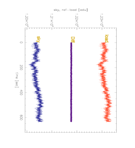
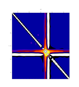
d)	e)	f)

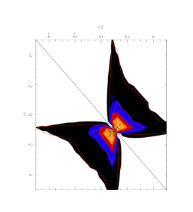
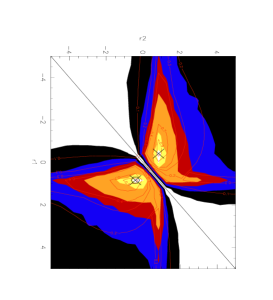
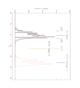
Figure 10: Example of signal for the detector 2300 acquired during the tests and its optimization. Frame a: are the sky and reference–load and $\Delta T$ samples in analog–to–digital units (ADU). The differentiated signal has been shifted up, having null mean. Relevant statistics are reported in Tab. 2a. Frame b: represents the accuracy by which the analytical model is able to predict the entropy measured on the quantized signal as a function of $r1$ and $r_{2}$ for $q=1$. Contours of regions are for accuracies of 0.5%, 1%, 1.5%, 2%, 2.5%. White boxes denote the regions where an accuracy worst than 3% is obtained by the simplest analytical model. Outside these regions the two models are completelly equivalent. Frame c: represents the accuracy by which the most sophisticated analytical model presented in Appendix A is able to predict the $C_{\mathrm{r}}$ for $q=1$. Contour lines are for accuracies of 5%, 10%, 15%, 20%, 25%, and 30%. Frame d: compares $\Gamma_{\mathrm{diff}}$ for the analytical model with $\Gamma_{\mathrm{diff}}$ computed for the numerical model. Colours are for $\Gamma_{\mathrm{diff}}$ analytical equal to 0.1, 0.2, 0.3, 0.4, 0.7, and 0.9 while contours are for the same values of $\Gamma_{\mathrm{diff}}$ numerical. The black hexagon identifies the regions for the peaks of $\Gamma_{\mathrm{diff}}$ analytical, the crosses for the peaks of $\Gamma_{\mathrm{diff}}$ numerical. Frame e: the same as of Frame d, but for $\Gamma_{\mathrm{sky}}$. Frame f: in black on the left, the histogram of $C_{\mathrm{r}}$ obtained on the 111 packets produced by the compression procedure with the optimized parameters of Tab. 2b. The figure gives also the 5% and 95% percentiles (p05 and p95) and the mean, and in red a gaussian fit of the histogram. In addition the figure shows in red at the right the $C_{\mathrm{r}}$ expected from the entropy directly measured on each packet, and the theoretical compression rate expected from the theroretical model (CrTh) and from the entropy measured on the whole quantized TOI.

Table 2: Table for the optimization example illustrated in Fig. 10. Subtable A) reports sky and reference–load statistics together with their correlation, and the derived $r$ and $R_{\sigma}$. Subtable B) reports the optimized REBA parameters, obtained respectivelly with the analytical approximation, and subsequently with a numerical scan of the parameter space. The processing statistics are reported in the Subtable C) where the processing errors and the $C_{\mathrm{r}}$ expected from the analytical model are compared with the numerical results. The third column of the subtable gives the theoretical expectations after replacing $q$ obtained from theory with $q$ obtained by numerical means.

	A) TOI Statistics
	sky	reference–load	Combined
Mean [adu]	12041.29	12313.63
RMS [adu]	9.72	10.06
Slope [adu/sec]	0.026	0.027
$\varrho_{\mathrm{s}\mathrm{l}}$			0.9988
$r$			0.9779
$R_{\sigma}$			0.9659
RMS($\Delta T)$ [adu]			1.45
	B) Optimized Parameters
	Analytical	Numerical
$r1$	1.25	1.25
$r2$	0.83	0.83
$\mathcal{O}$	785.41	784.39
$q$	0.203	0.317
	C) Processing Statistics
	Analytical	Numerical	Analytical with numerical $q$
$N_{\mathrm{pck}}$	97	111	–
$\Delta_{\mathrm{distr}}$	479.1	478.9	–
$\sigma_{1}$ [adu]	3.291	3.292	–
$\sigma_{2}$ [adu]	1.885	1.884	–
$\epsilon_{q,\mathrm{diff}}$ [adu]	0.043	0.067	0.068
$\epsilon_{q,\mathrm{sky}}$ [adu]	0.211	0.330	0.329
$\epsilon_{q,\mathrm{load}}$ [adu]	0.199	0.310	0.311
$(\sigma/q)_{\mathrm{eff}}$	9.7	6.2	6.2
$\max(|\mathcal{Q}_{\mathrm{ack}}|)$	0.388	0.228	0.248
$H_{\mathrm{Tot}}$ bits	6.667	6.023	6.021
Mean $H$ bits	–	5.489	–
Mean $\eta_{\mathrm{oca2k}}$	–	0.828	–
Min $C_{\mathrm{r}}$	–	2.286	–
5% $C_{\mathrm{r}}$	–	2.333	–
Median $C_{\mathrm{r}}$	–	2.413	–
Mean $C_{\mathrm{r}}$	2.4	2.414	2.657
95% $C_{\mathrm{r}}$	–	2.469	–
Max $C_{\mathrm{r}}$	–	2.510	–
RMS $C_{\mathrm{r}}$	–	0.045	–

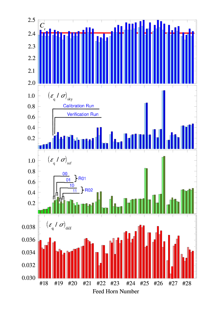
Figure 11: Results for a typical session of REBA parameters tuning during the CSL test campaign. From top to bottom the figure reports for each detector the mean $C_{\mathrm{r}}$, $\epsilon_{q,\mathrm{sky}}/\sigma_{\mathrm{sky}}$, $\epsilon_{q,\mathrm{load}}/\sigma_{\mathrm{load}}$, $\epsilon_{q,\mathrm{diff}}/\sigma_{\mathrm{diff}}$ where $\sigma_{\mathrm{diff}}$ is the r.m.s. of the differentiated data. The red line in background of the top frame denotes the target $C_{\mathrm{r}}^{\mathrm{Tgt}}=2.4$. Values are represented by bars. Light–bars are the results from the calibration phase, where raw data from the instrument are processed by OCA2. Dark–bars are results from the verification phase, where processing is performed on–board. The second frame from Top gives an example for detector 00 of Feed–Horn #19. Feed–horns are numbered according to the internal Planck/LFI convetion assigning at Planck/LFI the Feed–Horns numbers from #18 to #28. Detectors belonging to the same Feed–Horn are grouped together as shown in the third frame from top.

4 Results

As an exemplificatio, the results of REBA calibration and optimization in the framework of the Planck/LFI ground tests are presented here. First a single test is analyzed to compare the analytical and the numerical optimizations. After that the results of the calibration for the whole set of 44 detectors are presented for a real case.

The results of analytical v.z. numerical optimisation are compared by using real Planck/LFI data acquired during the RAA tests of the instrument performed at Thales Alenia Space (Italy), during the summer of 2006. Fig. 10a shows 12 min of data with $N_{\mathrm{aver}}=52$, equivalent to about 56715 samples, while Tab. 2a gives the relevant statistics for the TOI. During the test the instrument and its environment were stable, no strong drifts are present in the data. A clear correlation between sky and reference–load is evident in the plot explaining the $\varrho_{\mathrm{s}\mathrm{l}}\approx 1$ and the factor of six reduction of the RMS when passing from undifferentiated to differentiated data. Also the separation between sky and reference–load is not large being just 18$\sigma$. So after mixing the distributions for $\mathcal{P}_{1}$ and $\mathcal{P}_{2}$ will stay well separated, with $|\Delta_{\mathrm{distr}}|>100$, when $|r_{2}-r_{1}|\gtrsim 0.2$. In this case it is reasonable to expect that both the low–accuracy and high–accuracy methods to estimate analytically the entropy will give comparable results.

Indeed, both models to optimize the REBA parameters for $C_{\mathrm{r}}^{\mathrm{Tgt}}=2.4$, give exactly the same results as shown in the second column of Tab. 2b and Tab. 2c.

To test the goodness of the AO, OCA2K was run imposing $q=1$ and taking the same values of $r1$, $r2$ used for the AO. The predicted entropy of the processed TOI is compared in Fig. 10b. There the relative difference between the entropy measured all over the TOI and the entropy computed analytically by using both methods is reported. Patches define intervals of accuracy in steps of $0.5\%$ up to $3\%$. Both methods to estimate the entropy are good predictors of the measured entropy, apart from the region marked with the white boxes where the low accuracy method overestimated the entropy.

In a similar manner in Fig. 10c the measured $C_{\mathrm{r}}$ and the predicted from the high accuracy model are compared. Again the model is able to reproduce within $20\%$ or better the measured $C_{\mathrm{r}}$. As discussed before the differences can be ascribed mainly to the difference between the sampling entropy and the expected entropy ([Maris et al. (2000)]) and the not–ideal behavior of the compressor ([Maris et al. (2000)]). In general the effect of the sampling entropy would result in a higher $C_{\mathrm{r}}$ than expected while non idealities in a lower $C_{\mathrm{r}}$. Different ways can be used to calibrate these effects, however their interplay with the statistic of the signal is complicated and it is preferable to use OCA2K to fine tune the REBA parameters optimized by analytical mean, given that in general the corrections required to properly tune with respect to the analytical prediction $q$ are at most of about a factor of two.

The numerically refined optimal parameters are reported in the third column of Tab. 2c, as it is evident the only variation is just for $q$, the reason is explained by the contour plots in Fig. 10d and Fig. 10e which compares the predicted analytical $\Gamma_{\mathrm{diff}}$ and $\Gamma_{\mathrm{sky}}$ with the $\Gamma_{\mathrm{diff}}$ and $\Gamma_{\mathrm{sky}}$ obtained for the numerically refined parameters. Very good agreement is obtained in the location of the peaks which determines the optimal $r_{1}$, $r_{2}$ and in turn the $\mathcal{O}$. For completeness the last column of Tab. 2d reports the theoretically estimated $\mathcal{Q}_{\mathrm{ack}}$, $\epsilon_{q,\mathrm{diff}}$, $\epsilon_{q,\mathrm{sky}}$ and $\epsilon_{q,\mathrm{load}}$ after replacing the analytical optimal $q$ with the numerical one. The very good agreement between the theory and the experiment is evident.

As expected the quantization error for the differentiated data is smaller by about a factor of four than the error for sky or reference–load and anyway the error will be a fraction of ADU, but larger or comparable to the quantization error introduced by the ADC converter, which for $N_{\mathrm{aver}}=52$ is equivalent to $\approx 0.04$ ADU.

Eq. (24) expresses the processing error for an univariate normal distribution as a function of the $\sigma/q$ ratio, but from Sect. 2.5 it is evident that in the present case the $\sigma/q$ ratio is not a good measure of the processing error. At the opposite, it is possible to define an effective $\sigma/q$ ratio in terms of the processing error as

$$\left(\frac{\sigma}{q}\right)_{\mathrm{eff}}=\frac{\sigma_{\mathrm{diff}}}{\sqrt{12}\epsilon_{q,\mathrm{diff}}};$$ (94)

which expresses the number of independent quantization levels which could be accommodated within $1\sigma$. So this ratio gives an idea of how well the histogram of the differentiated data is sampled assuming it could be represented by an univariate normal distribution . A proper sampling would assure at least $(\sigma/q)_{\mathrm{eff}}>2$ which is the case for this work as it is evident from Tab. 2c having $(\sigma/q)_{\mathrm{eff}}>6$.

Before concluding this comparison it is worth commenting the way in which the experimental $C_{\mathrm{r}}$ is reported in Tab. 2c. This is best done by looking at Fig. 10f where the histogram for the $C_{\mathrm{r}}$ of the 111 packets produced in the test is shown. Given the true $C_{\mathrm{r}}$ is a random variable, varying from packet to packet we take the $5\%$ and $95\%$ percentiles assessing that in less than $5\%$ the $C_{\mathrm{r}}$ will be respectively smaller or larger than the quoted $C_{\mathrm{r}}$, as well as the mean and the median (not quoted in the figure) of the measured $C_{\mathrm{r}}$. In this case it is evident that the target $C_{\mathrm{r}}{\stackrel{{{}_{>}}}{{{}_{\sim}}}}2.4$ is achieved in something less than half of the packets. So it would be better to introduce some safety factor, as an example by requiring $C_{\mathrm{r}}^{\mathrm{Tgt}}\approx 2.6$ or by requiring the median be $C_{\mathrm{r}}$ to be 2.4, or better by asking the 5% percentile of the $C_{\mathrm{r}}$ distribution to be $\approx 2.4$.

Fig. 11 is representative of the results of the calibration for a whole set of 44 detectors obtained during the Planck/LFI CSL test campaign in 2008 [Cuttaia at al.(2009)]. Data have been collected over two acquisitions, the first one being used for the calibration itself and the second one to verify the calibration performances. The environmental set-up and the onboard electronics were kept in a stable state during both acquisitions. During the first acquisition, called “calibration run”, the on–board computer was configured to apply just the downsampling step to the data but skipping mixing, requantization and compression. The acquired data have been ingested into OCA2K to generate a list of optimized processing parameters for a target $C_{\mathrm{r}}=2.4$. Having obtained a set of parameters for the REBA, the second acquisition, the “verification run”, while the instrument was set up to acquire data in nominal conditions, by using the same processing steps that are going to be used during flight. At the same time data have been also acquired in the raw format used in the “calibration run”. So for each detector couples of data streams with and without on–board processing were obtained which have been compared in order to measure the processing error, following a procedure similar to the one described in [Fraillis et al. (2008b)].

Fig. 11 compares the mean $C_{\mathrm{r}}$, $\epsilon_{q,\mathrm{sky}}/\sigma_{\mathrm{sky}}$, $\epsilon_{q,\mathrm{load}}/\sigma_{\mathrm{load}}$, $\epsilon_{q,\mathrm{diff}}/\sigma_{\mathrm{diff}}$, where $\sigma_{\mathrm{diff}}$ is the r.m.s. for the differentiated data. Bars in light colours are for results obtained by processing the data taken in the calibration run with the OCA2 simulator. Bars in dark colours are the results from the data processed by the instrument in the verification run. In both cases the same set of optimal REBA parameters have been used. There is good agreement between the two runs, despite the presence of a few systematics. Such differences are due to slight changes in the environmental conditions between the two runs . Differences in channels belonging to the same radiometer (00 and 01, 10 and 11) are due to the fact that in the warm back end the two channels go through separate acquisition lines, each of them being characterized by different noise properties [Bersanelli et al. (2009)]. Such differences are usually small, e.g. detectors (00, 01) and (10, 11) of Feed–Horn #19. In a few cases however larger differences occurs, e.g. detectors (10, 11) of Feed–Horn #25. Again, the relative processing errors for sky and reference–load are very similar, and in 95% of the detectors they are below 0.4 with some extreme deviations such as detectors 10 of Feed Horn #25 and 11 of Feed Horn #26 for which $\epsilon_{q,\mathrm{sky}}/\sigma_{\mathrm{sky}}\approx\epsilon_{q,\mathrm{load}}/\sigma_{\mathrm{load}}{\stackrel{{{}_{>}}}{{{}_{\sim}}}}1$. Here the optimal $q_{\mathrm{opt}}$ is not peculiar with respect to the values required for the other detectors, but optimal $r_{1}$ and $r_{2}$ are very similar having $|r_{2}-r_{1}|=0.04$ which is the resolution of the search grid in the $(r_{1},r_{2})$ space. Such relativelly “coarse” resolution in the search grid for optimal $(r_{1},r_{2})$ was imposed by constraining the need to optimize the REBA parameters within a few minutes after the data acquisition. The coarseness of the $(r_{1},r_{2})$ grid is also the reason for the apparent coincidence of the mean values of $r_{1}$ and $r_{2}$ for different frequency channels in Tab. 3. In flight such time constraints will be removed allowing a multi step iteration of the optimization procedure and the use of a thinner grid. However, even in those extreme cases, the coorrelation between sky and reference–load processing errors leads to a much smaller error for the differentiated data. In all cases the final processing error is always less than $3.8\%$ of the instrumental white noise. Scaling those numbers to the calibrated sensitivity per sample and per detector, the calibrated processing error, $\Delta T_{q}$, was derived, and is reported in units of $\mu\mathrm{K}$ per sample and per detector in line 10 of Tab. 3. On average $\Delta T_{q}$ is below the 3 $\mu\mathrm{K}$ level taken as a threshold for systematics [Mandolesi et al. (2009)] apart from the detector 01 of the Feed–Horn #24 for which $\Delta T_{q}\approx 3.2$ $\mu\mathrm{K}$.

The values for the optimal REBA parameters are mainly determined by the frequency of the radiometric channel with some dispersion from detector to detector. Tab. 3 gives representative median values for $r_{1}$, $r_{2}$, $q=1/S_{\mathrm{q}}$ from the CSL tests as well as for the quantities in Fig. 11 and the resulting data rate. $\mathcal{O}$ is omitted since it is the most variable parameter and it has no significative impact on $\epsilon_{q}$ and $C_{\mathrm{r}}$. Tab. 3 reports also the number of detectors for each frequency channel, the $N_{\mathrm{aver}}$ values which are kept constant, the compressed data rate per detector, per frequency channel and for the instrument as a whole. Quantities are reported in the form $x\pm\delta x$ where $\delta x$ represents the standard deviation taken as a measure of the internal dispersion of $x$ within the given subset of detectors. Of course this number must not be interpreted as an error and it must not be propagated.

The total data–rate in Tab. 3 is just 7% higher than the target data–rate 35.5 bits/sec. Again this departure is mainly due to the limited resolution in the search grid as well as small changes in the environmental conditions between the two runs. In order to cope with this problem it is likely that during operations a safer $C_{\mathrm{r}}^{\mathrm{Tgt}}=2.5$ target will be set in place of the nominal 2.4.

Finally it is worth to consider the gain in the accuracy of the REBA optimization obtained by the complex procedure described in Sect. 3 with respect to the fairly simple scheme used in the earlier RAA test campaign [Bersanelli et al. (2009)]. During the RAA tests a simplified algorithm had been applied based on the fact that putting $r_{1}=r$ the processing error for the differentiated data reduces to Eq. (64) which is independent of $r_{1}$ and $r_{2}$. Hence, the only free parameters where $q$ and $r_{2}\neq r$. The optimization was performed by imposing $C_{\mathrm{r}}=2.4$ and selecting those parameters for which $\epsilon_{q,\mathrm{sky}}\approx\epsilon_{q,\mathrm{load}}\approx\epsilon_{q,\mathrm{diff}}$. Even in this case the required $Cr=2.4$ was achieved but $\epsilon_{q,\mathrm{diff}}/\sigma_{\mathrm{diff}}$ was between $[0.08,0.14]$, when compared to the current $\epsilon_{q,\mathrm{diff}}/\sigma_{\mathrm{diff}}\leq 0.038$ it is evident how this procedure represents a substantial improvement. In particular LFI has as a target of keeping all of the instrumental systematics and non gaussian noises in the differentiated data below 10% of the instrumental white noise [Bersanelli et al. (2009)]. The optimization scheme described here allows the reduction of the processing error on the differentiated data by a factor of four pushing it below this ambitious target.

Table 3: Representative REBA Parameters, the measured $C_{\mathrm{r}}$ and relative processing errors from the CSL tests for Planck/LFI. Detectors are grouped by frequency channel, for each quantity $x$ the table reports its group median and group standard deviation $\delta x$ as a measure of the group internal dispersion, $\delta x$ must be not considered as an error.

	Frequency Channel
	30 GHz	44 GHz	70 GHz
Detectors	8	12	24
$N_{\mathrm{aver}}$	126	88	53
$r_{1}$	$1.042\pm 0.032$	$1.042\pm 0.024$	$1.042\pm 0.012$
$r_{2}$	$0.917\pm 0.065$	$0.917\pm 0.025$	$0.958\pm 0.020$
$q$ [adu]	$0.297\pm 0.034$	$0.198\pm 0.044$	$0.279\pm 0.048$
$C_{\mathrm{r}}$	$2.400\pm 0.024$	$2.440\pm 0.019$	$2.380\pm 0.023$
$\left({\epsilon_{q}}/{\sigma}\right)_{\mathrm{sky}}$	$0.420\pm 0.278$	$0.269\pm 0.184$	$0.177\pm 0.063$
$\left({\epsilon_{q}}/{\sigma}\right)_{\mathrm{load}}$	$0.432\pm 0.267$	$0.271\pm 0.183$	$0.178\pm 0.063$
$\left({\epsilon_{q}}/{\sigma}\right)_{\mathrm{diff}}$	$0.0341\pm 0.0016$	$0.0369\pm 0.0010$	$0.0351\pm 0.0010$
${\Delta T_{q}}$ [$\mu\mathrm{K}$]	$1.759\pm 0.148$	$2.412\pm 0.356$	$1.905\pm 0.287$
Data Rate per Detector [bits/sec]	$454.9\pm 4.1$	$640.8\pm 4.7$	$1108.2\pm 9.8$
Data Rate per Frequency Channel [bits/sec]	$3641.8$	$7689.9$	$26600.3$
Total Data Rate [bits/sec]	37932

a)	b)
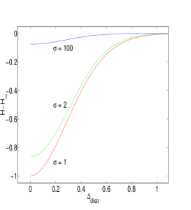
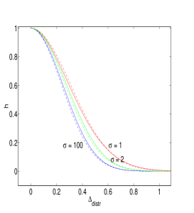
c)	d)

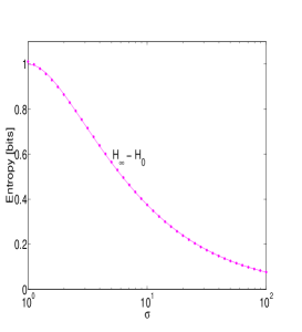
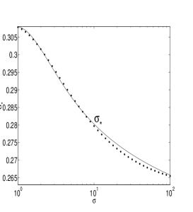
Figure 12: Frame a: Entropy variation for a couple of normally distributed signals as a function of $\Delta_{\mathrm{distr}}$ for three values of $\sigma$. The reference entropy is ${H_{\infty}}$. Frame b: Normalized entropy for a couple of normally distributed signals as a function of $\Delta_{\mathrm{distr}}$ for three values of $\sigma$. Full lines: numerical integration. Frame c: Normalized entropy difference ${H_{\infty}}-{H_{\mathrm{min}}}$ as a function of $\sigma$ for a couple of normally distributed signals. Full lines: numerical integration. Dots: approximated formula. Frame d: The $\sigma_{*}$ parameter as a function of $\sigma$ for a couple of normally distributed signals. Full lines: numerical integration. Dots: approximated formula.

5 The impact of the on–board processing noise on the Planck scientific performances

A detailed analysis of the effect of on–board plus on–ground processing on the final scientific products of Planck is beyond the scope of this paper. The subject is simply too complex to be analyzed here, and the analysis has to be specialized to take into account each specific kind of product obtained from the Planck data i.e.: calibrated time lines, frequency maps, component maps, angular power spectra for those maps and cosmological parameters. Neglecting in this discussion the role of $r_{1}$ and $r_{2}$ it is enough to say that for most of these products the effect of processing could be reduced to the effect of processing on the signal spectral decomposition in the time or in the spatial domain. Without to enter in to too many details, some consideration could be derived from the analysis reported in [Maris et al. (2004)] and from a forthcoming work in progress [Maris et al. (2009)].

In the extent in which the processing error for differentiated data is small when compared to the fluctuations in the signal, the noise model for the quantization error data could be applied to derive the level of degradation in the noise properties of the instrument. In the Planck/LFI case, for differentiated data a typical $(\epsilon_{q,\mathrm{diff}}/{\sigma_{\mathrm{wn}}})<0.1$ by using Eq. (7) of [Maris et al. (2004)] the final instrumental performances will be degraded approximately by a factor $\sqrt{1+(\epsilon_{q,\mathrm{diff}}/{\sigma_{\mathrm{wn}}})^{2}}<1.01$. This immedialty applies to the amplitudes of the spectral decomposition of the signal. Since processing acts as stationary white noise it will increase by less than $1\%$ the power excess introduced by the white noise. On the other hand the effect on the phases will be similar to to random scrabling over the $[0,2\pi]$ interval, but even in this case the effect of quantization will be to increase by few percent the effect of the instrumental white noise. It is immediately possible to extend these results to the Planck/LFI calibration which will be based on measurents of the amplitude of the cosmological dipole, to understand how, when compared to the white noise effect, the calibration accuracy will be worsened by less than $1\%$ by the processing noise.

It is more complex to consider the case of the Planck/LFI sensitivity to primordial non–gaussianities. In [Maris et al. (2004)] the level of perturbation the measurements of primordial non–gaussianities introduced by the quantization were compared to the level of perturbation introduced by the residuals astrophysical foregrounds concluding that they are very small. However, it is worth analyzing the effect of processing on non–gaussianities even assuming an ideally perfect separation of the foregrounds. To the extent that the quantizer has null expectation, null skewness and in general null central moments of odd order, no effect is expected on tests of primordial non–gaussianity which are sensitive just to central moments of odd orders. Of course a symmetrical quantizer will alter the central moments of even order, such as the kurtosis. To estimate this effect it is sufficient to compare the distribution of the processing noise from a uniform quantizer with the case of normal white noise while taking the average over $N$ repeated measures. In the white noise case the central moments of even order are $\mu_{n}=C_{g}(n)\sigma^{n}/N^{n/2}$, with $C_{g}(n)=n!/(2^{n/2}*(n/2)!)*s^{(}n)$. In the case of the quantizer $\tilde{\mu}_{n}(N,q)=\tilde{C}(N,n)(q/\sqrt{12})^{n}/N^{n/2}$, whatever the form of $\tilde{C}(N,n)$ is the Central Limit Theorem assures that for any $n$

$$\lim_{N\rightarrow\infty}\tilde{C}(N,n)=C_{g}(n).$$

but given $N$ is finite, a bias in the estimator for each moment of order $n$ will appear. Expanding $\tilde{C}(N,n)$ about $1/N$ up to the leading term

$$\tilde{C}(N,n)\approx C_{g}(n)\left(1+\frac{A_{n}}{N^{n/2-1}}\right),$$

where $A_{n}$ is a serie of coefficients having $|A_{n}|<1$ whose first three elements are $A_{2}=0$, $A_{4}=-2/5$, $A_{6}=-6/5$, $A_{8}=-12/7$. Since for Planck/LFI $N\approx 60$ the bias in the expectation of higher order moments will be very small. In addition, since $N$ is a characteristic parameter of a mission, any bias due to processing in the estimators of central moments could be predicted and removed.

In closing these considerations it is worth noting that for Planck/LFI the most important limitation to apply an hard requantization of data comes from the need to limit the effect on the total power data rather than on the differential data. Firstly it has to be noted that the cancellation effect of quantizzation errors on sky and reference–load from which Eq. (62) is derived, applies only to the $(P_{1},P_{2})$ space of mixed data to the extent in which $q/\sigma_{i}<\sqrt{12}/3$ for any $i=1$, 2. Another limit in the maximum amount of processing noise which could be introduced in total power arises when it is taken in consideration the fact that measurements in total power on the reference–load signal have the potential to be a valuable tool as a source of diagnostics of instrumental systematics. An example is given by the study of thermal effects induced by the instability of the reference–load which could be detected by cross–correlating ${T_{\mathrm{load}}}$ with measurements of temperatures acquired by thermometers located in the Planck focal plane, which limits the quantization on ${T_{\mathrm{load}}}$ to be $\epsilon_{q,\mathrm{load}}/\sigma_{\mathrm{load}}\leq 1/2$ [Maris et al. (2009)].

6 Final Remarks and Conclusions

As for many past, present and future scientific space missions, the ESA Planck mission has a limited bandwidth to download the scientific data produced by its two instruments. The allocatable bandwidth for the Planck/LFI is about 2.4 times lower than the raw data flow produced by the 44 detectors comprising the instrument, which is made of an array of 22 pseudo–correlation receivers, each one comparing the signal received from the sky with a reference signal. To fit the allocated bandwidth data have to be preprocessed on-board and loss–less compressed prior to transfer to the ground, where each step of the on–board preprocessing has to be reversed to recover the original information. Since not all of these steps are completely reversible, a overall reduction of the quality of the data occurs, which has to be quantified and reduced as more as possible, not to degrade the instrument performace.

This paper has presented a detailed discussion of the on–board plus on–ground processing for Planck/LFI and of its free parameters which can be adjusted in order to fit the compressed data–rate to the allowed bandwidth. In addition, this paper has presented a model to quantify the level of distortion in the scientific data as a function of the free parameters for the on–board processing and as a function of the attainable compression rate. At last the paper has reported on the way these parameters are optimized to cope with the required bandwidth while limiting the processing distortion.

Three new results about the way in which the output of a pseudo–correlation receiver could be handled are presented. First, a new algorithm: mixing followed by requantization and interlacing to prepare the data stream for compression, limiting at the same time the amount of processing distortion is introduced. This method is effective, since most of the time variations in the sky and reference–load data streams are correlated. Mixing reduces the effective variance of the signal to be compressed therefore relaxing the need for requantizing the data. At the same time the processing errors in the mixed data are correlated, so that on ground demixing introduces cancellation effects which reduce the re–quantization error in the differentiated signal. Second, a model which quantifies the level of distortion in the scientific data as a function of the free parameters of the on–board processing and as a function of the attainable compression rate is given. Third, it presents a general procedure to search for optimized processing parameters which has to cope with the proper use of the allocated bandwidth, requiring a nominal compression factor of 2.4, which has to limit as much as possible the processing distortion, and has to be fast given that both in the pre–launch tests campaign and in flight only a short time could be allocated for optimization.

The optimization procedure is based on a combination of the analytical model and of a software simulator, all integrated into a single applicative program called OCA2 which takes as input a Planck/LFI data stream applying to it the whole on–board and on–ground processing to measure the processing distortion and the data–rate. The two approaches complement each other: the analytical model is very fast and could be used to rapidly select regions of interesting combinations of parameters; the simulator is able to handle conditions which hardly can be analytically modelled and is used to refine the parameters identified by the analytical model. The input data for OCA2 can be provided indifferently by the Planck/LFI flight simulator [Reineker, Dolag (2006)], or from specific acquisition sessions performed during the test campaign or in flight. A wide selection of combinations of processing parameters and optimization criteria can be explored by this code. In practice this work shows that the analytical model is refined enough to allow a full optimization of all of the processing parameters apart from the on–board re–quantization step, $q$, which has to be tuned numerically to account for a number of non–idealities in the data and in the compressor, part of which have been discussed in the paper. However, it is interesting to see that in no cases there are no situations where the difference between the analytical and the numerical model in the optimized $q$ is larger than a factor two.

The last part of this work reports the performances of the optimized on–board  algorithms in the framework of the pre–launch tests required for instrument qualification. In that case it has been demonstrated that the 2.4 compression factor required to operate Planck/LFI could be attained introducing a modest quantization noise equivalent to a 3.8% of the unprocessed signal rms, which is equivalent to an increment in the instrumental noise of less than $1\%$, in particular processing is not harmful to the scientific exploitation of Planck/LFI data such an example in the study of primordial non–gaussianities.

In conclusion it is worth noting that the application of mixing follwoed by requantization is of general use and could be extended outside the case of the Planck/LFI since it could be used in any situation in which data alternatively taken from a signal source and a reference source are sent to a remote station.

Appendix A Approximation of the bivariate entropy

This section presents the approximation of the entropy for an interlaced bivariate distribution for the two limiting cases of a uniform distribution or a normal distribution.

The case of two uniform distributions

The case of two uniform distributions is analyzed by defining the intervals where the distributions are not null as $Q_{1,\mathrm{l}}\leq Q_{1}\leq Q_{1,\mathrm{r}}$ and $Q_{2,\mathrm{l}}\leq Q_{2}\leq Q_{2,\mathrm{r}}$, and their widths $N_{1}=Q_{1,\mathrm{r}}-Q_{1,\mathrm{l}}$, $N_{2}=Q_{2,\mathrm{r}}-Q_{2,\mathrm{l}}$, their centers $\bar{Q}_{1}=(Q_{1,\mathrm{l}}+Q_{1,\mathrm{r}})/2$, $\bar{Q}_{2}=(Q_{2,\mathrm{l}}+Q_{2,\mathrm{r}})/2$. Without any loss of generality $N_{1}\leq N_{2}$ is assumed. The entropy is a linear function of $|\Delta|=\left|\bar{Q}_{2}-\bar{Q}_{1}\right|$ bounded between the lower limit

$${H_{\mathrm{min}}}=\frac{1}{2}\left(1-\frac{N_{1}}{N_{2}}\right)H_{2}-\frac{N_{1}}{2}\left(\frac{1}{N_{1}}+\frac{1}{N_{2}}\right)\log_{2}\left(\frac{1}{N_{1}}+\frac{1}{N_{2}}\right)+1,$$ (95)

in the case the two distributions are completely overlapped, and the upper limit

$${H_{\infty}}=\log_{2}N_{1}+\log_{2}N_{2}+1,$$ (96)

for the case of complete separation of the two distributions. So that

$$H=\left\{\begin{array}[]{ll}|\Delta|<\frac{N_{2}-N_{1}}{2},&{H_{\mathrm{min}}}\\ \frac{N_{2}-N_{1}}{2}\leq|\Delta|\leq\frac{N_{2}+N_{1}}{2},&({H_{\infty}}-{H_{\mathrm{min}}})\frac{2|\Delta|-N_{2}+N_{1}}{2N_{1}}+{H_{\mathrm{min}}}\\ \frac{N_{2}+N_{1}}{2}<|\Delta|,&{H_{\infty}}\\ \end{array}\right..$$ (97)

The case of two normal distributions

Whithout any loss of generality, it is possible to reduce to the case of two sources of normal–distributed interlaced signals having respectively variances equal to 1 and $\sigma^{2}\geq 1$, and quantized with a quantization step $q<1$.

An approximation for $H(\Delta_{\mathrm{distr}},q,\sigma)$ can not be derived analytically, but in a manner similar to the case of the uniform distribution the entropy is bounded between a lower limit, ${H_{\mathrm{min}}}$, and an upper limit ${H_{\infty}}$, while varying $\Delta_{\mathrm{distr}}$. In Fig. 12a shows how the entropy varies as function of $\Delta_{\mathrm{distr}}$ for three different values of $\sigma$. In addition both $H$, ${H_{\infty}}$ and ${H_{\mathrm{min}}}$ are proportional to $-\log_{2}q$ so that their differences does not depend on $q$. For this reason it is convenient to define the Normalized Entropy, $h$

$$h=\frac{H-{H_{\infty}}}{{H_{\mathrm{min}}}-{H_{\infty}}};$$ (98)

which is just a function of $\Delta_{\mathrm{distr}}$ and $\sigma$ as shown in Fig. 12b (as full lines) for three values of $\sigma$.

Having $h$, $H-{H_{\infty}}$ and $q$

$$H={H_{\infty}}-\log_{2}q+({H_{\infty}}-{H_{\mathrm{min}}})h,$$ (99)

note that there is not need to estimate ${H_{\mathrm{min}}}$, and that ${H_{\infty}}$ could be readily estimated from Eq. (100) by putting $\sigma_{1}=1$, $\sigma=\sigma_{2}/\sigma_{1}$, and expressing $q$ in units of $\sigma_{1}$.

The difference $({H_{\infty}}-{H_{\mathrm{min}}})\leq 1$ bit is always positive and just function of $\sigma$. It is null in the limit $\sigma\rightarrow+\infty$ as shown in Fig. 12c. The figure displays with a dotted line an approximation obtained numerically for $1\leq\sigma_{2}\leq 4000$ for which

$${H_{\infty}}-{H_{\mathrm{min}}}=\exp\left[\sum_{n=1}^{5}A_{n}(\log\sigma_{2})^{n}+A_{0}\right]$$ (100)

with $A_{0}=1.0893\times 10^{-2}$, $A_{1}=-8.3819\times 10^{-2}$, $A_{2}=-2.3699\times 10^{-1}$, $A_{3}=4.8141\times 10^{-2}$, $A_{4}=-5.1620\times 10^{-3}$, $A_{5}=2.1425\times 10^{-4}$ within an accuracy of $\pm 1.1\%$.

For $h$ a numerical approximation at the level of a $\pm 1\%$ accuracy is

$$h\approx e^{-\frac{\Delta_{\mathrm{distr}}^{2}}{2\sigma_{*}^{2}}}.$$ (101)

Here $\sigma_{*}$ is just a function of $\sigma$, and it is bounded between $0.25558\leq\sigma_{*}\leq 0.30797$ with an $\approx 21\%$ variation, as shown in Fig. 12d. An upper limit for $h$ is derived by putting $\sigma_{*}=0.30797$ overestimating the entropy of at most $(\sqrt{{H_{\infty}}-{H_{\mathrm{min}}}})0.16\leq 0.16$. However $\sigma_{*}$ is a function of $({H_{\infty}}-{H_{\mathrm{min}}})$ allowing to derive

$$\sigma_{*}=\sqrt{6.8497\times 10^{-2}+2.5965\times 10^{-2}({H_{\infty}}-{H_{\mathrm{min}}})}+\epsilon$$ (102)

with $|\epsilon|\leq 2\times 10^{-2}$. With this approximation the typical accuracy in estimating $H$ is better than $0.01\div 0.03$ bits and the optimal $q$ for a given $H_{\mathrm{tgt}}$ can be derived from

$$\log_{2}q_{\mathrm{opt}}=({H_{\mathrm{min}}}-{H_{\infty}})h+{H_{\infty}}-H_{\mathrm{tgt}},$$ (103)

within a relative numerical accuracy of about $3\%$.

In short, the algorithm of optimization becomes for given $r_{1}$, $r_{2}$, $q$, $\sigma_{1}$, $\sigma_{2}$, $T_{1}$, $T_{2}$ is: i.) compute $\sigma$, $\Delta_{\mathrm{distr}}$, ii.) compute $\sigma_{*}$, $h$, ${H_{\infty}}$, ${H_{\infty}}-{H_{\mathrm{min}}}$, iii.) compute $q_{\mathrm{opt}}$.

Appendix B ADC quantization

Throughout this work it is assumed that the ADC quantization is not relevant for the scopes of this paper. However, it is worth to briefly recall its impact, in particular looking at the conditions at which the ADC noise could be neglected.

The resolution, or quantization step of the ADC, ${q_{\mathrm{ADC}}}$ is given by $(V_{\mathrm{max}}-V_{\mathrm{min}})/2^{14}$ Volts/ADU, after averaging by $N_{\mathrm{aver}}$ samples ${q_{\mathrm{ADC}}}$ is reduced by a factor $1/\sqrt{N_{\mathrm{aver}}}$. The effect of the ADC resolution is to add in quadrature a non–Gaussian noise to the signals of RMS $1/\sqrt{12}$ before averaging and $1/\sqrt{12N_{\mathrm{aver}}}$ after averaging. In addition the ADC itself adds a random read–out noise of $\sigma_{\mathrm{ADC}}$ ADU which after averaging is reduced to $\sigma_{\mathrm{ADC}}/\sqrt{N_{\mathrm{aver}}}$. When combined these two noises the readout noise whose RMS is $\sigma_{\mathrm{ron}}=\sqrt{1/12+\sigma_{\mathrm{ADC}}}$ before averaging and $\sigma_{\mathrm{ron}}=\sqrt{1/12+\sigma_{\mathrm{ADC}}}/\sqrt{N_{\mathrm{aver}}}$ after averaging.

When a signal of RMS $\sigma_{0}$ is input to the DAE a gain, $G$, is applied and then the measured RMS is

$$\sigma=\sqrt{\sigma_{\mathrm{ron}}^{2}+G^{2}\sigma_{0}^{2}},$$ (104)

depending on the ratio $\sigma_{\mathrm{ron}}/G\sigma_{0}$. The measured RMS will be dominated by the ADC noise or by the signal RMS. Signals whose RMS is comparable to the read–out noise are defined as weak signals. Of course in the case of weak signals the read–out noise is no more negligible when, as an example, the $\sigma_{0}$ has to be measured in order to estimate the ${T_{\mathrm{sys}}}$. The same is true when the variation of the RMS of the signal tacking in account of variations of $G$ has to be estimated [Cuttaia at al.(2009)]. In addition, given the 1/12 factor in front of the variance induced by the ADC contribution, the read–out noise could be dominated by the ADC noise when $\sigma_{\mathrm{ADC}}>0.3$. As a practical example if $\sigma_{\mathrm{ADC}}\approx 0.5$ and $\sigma_{0}\approx 1$ then $\sigma_{\mathrm{ron}}\approx 0.57$ and the bias in estimating $\sigma_{0}$ will be $\approx 15\%$.

Appendix C DAE Tuning

In an ideal scheme of operations, the various stages of a complex instrument such as Planck/LFI would have to be calibrated sequentially, so that the calibration of the REBA parameters would be the last step of the calibration procedure [Cuttaia at al.(2009)] and would have no effect on the previous stages of calibration. Practical experience has shown that there is a case in which the tuning of the acquisition electronics has consequences on the subsequent tuning of the REBA parameters. Indeed, the hypothesis at the root of the whole compression scheme is that the noise variance of the input signal is large. This is in general true but this hypothesis could fail if the variance of the signal after ADC quantization, on–board coadding and mixing becomes too small. In that case the signal will be over compressed with $C_{\mathrm{r}}>C_{\mathrm{r}}^{\mathrm{Tgt}}$ and the squared quantization error will be larger or equal to the signal variance. To avoid this case either the DAE gain $G$ and $N_{\mathrm{aver}}$ have to be properly tuned, or a set of particular combinations of $r_{1}$, $r_{2}$ values has to be excluded.

The problem is to ensure $\sigma_{1}$ and $\sigma_{2}$ to be greater than a minimal $\sigma_{\mathrm{tgt}}$ typically assumed to be at least $2$ $\mathrm{adu}$ in a suitable range of $r_{1}$, $r_{2}$ values. From Eq. (39) it is evident that the $\sigma_{i}^{2}$ as a function of $r_{i}$ defines two identical concave parabolas with a minimum in $r_{1}=r_{2}=r_{\mathrm{min}}=\sigma_{\mathrm{sky},\mathrm{load}}/\sigma_{\mathrm{load}}^{2}$, where both $\sigma_{1}$ and $\sigma_{2}$ takes the value

$$\sigma_{\mathrm{min}}=\sigma_{\mathrm{sky}}\sqrt{1-\varrho_{\mathrm{s}\mathrm{l}}^{2}},$$ (105)

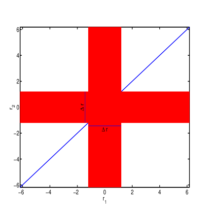
Figure 13: The region of the $r_{1}$, $r_{2}$ space excluded by the condition $\sigma_{1},\sigma_{2}>\sigma_{\mathrm{tgt}}$, red. The width of the two crossing bands, $\Delta r$, is given by Eq. (108). In this case $f_{\mathrm{DAE},\mathrm{excl}}\approx 0.35$.

where $\varrho_{\mathrm{s}\mathrm{l}}$ is the correlation coefficient between sky and reference–load. Note that $\sigma_{\mathrm{min}}=0$ just as in the case of a perfect correlation between sky and reference–load. So a sufficient condition to asses proper DAE calibration is

$$\sigma_{\mathrm{tgt}}<\sigma_{\mathrm{sky}}\sqrt{1-\varrho_{\mathrm{s}\mathrm{l}}^{2}},$$ (106)

which puts a constraint on the minimum $G/\sqrt{N_{\mathrm{aver}}}$ which could be accepted. In particular assuming the quantization and the readout noise are small with respect to the sky and reference–load RMS, at first order

$$\frac{G}{\sqrt{N_{\mathrm{aver}}}}>\frac{\sigma_{\mathrm{tgt}}}{{\sigma_{\mathrm{sky}}}_{,0}\sqrt{1-\varrho_{\mathrm{s}\mathrm{l}}^{2}}},$$ (107)

where ${\sigma_{\mathrm{sky}}}_{,0}$ is the sky RMS with $G=1$ and no averaging is applied.

It could happen that in some cases the condition (107) can not be full–filled for any reasonable value of $G$ and $N_{\mathrm{aver}}$. So a forbidden region in the $r_{1}$, $r_{2}$ space is defined by the need to have $\sigma_{\mathrm{tgt}}<\mathrm{min}(\sigma_{1},\sigma_{2})$. This defines a “cross” centered into $r_{1}=r_{2}=r_{\mathrm{min}}=\sigma_{\mathrm{sky},\mathrm{load}}/\sigma_{\mathrm{load}}^{2}$, see Fig. 13, with “harms” parallel to the two axis of the $r_{1}$, $r_{2}$ space and having for each harm a width

$$\Delta r=2\frac{\sigma_{\mathrm{sky}}}{\sigma_{\mathrm{load}}}\sqrt{\left(\frac{\sigma_{\mathrm{tgt}}}{\sigma_{\mathrm{sky}}}\right)^{2}-(1-\varrho_{\mathrm{s}\mathrm{l}}^{2})}.$$ (108)

During DAE calibration, the operators could monitor the evolution of $\Delta r$ as $G/\sqrt{N_{\mathrm{aver}}}$ varies. In general the optimization of $r_{1}$ and $r_{2}$ is performed by scanning a rectangular region in the $(r_{1},r_{2})$ space of limited width, thus an informative parameter to avoid to prevent a proper REBA calibration after DAE calibration is to check the fraction of area of the region of interest excluded by the DAE calibration $f_{\mathrm{DAE},\mathrm{excl}}$. It is not possible of course to write a general formula for all the possible cases, but if $\varrho_{\mathrm{s}\mathrm{l}}^{2}$ is small, the excluded region has a center near $r_{1}=r_{2}=0$, while the optimization region is a square, centered on the origin with $-r_{\mathrm{lim}}\leq r_{1},r_{2}\leq+r_{\mathrm{lim}}$ in that case

$$f_{\mathrm{DAE},\mathrm{excl}}=\frac{(4r_{\mathrm{lim}}-\Delta r)\Delta r}{4r_{\mathrm{lim}}^{2}}.$$ (109)

References

- [Bertotti, Farinella, Vokrouhlický (2003)] Bertotti, B., Farinella, V., Vokrouhlický, D., Physics of the Solar System: Dynamics and Evolution, Space Physics, and Spacetime Structure, Chapter. 19, 2003, Kluwer Academic Publishers, Dodrecht, The Netherlands, ISBN 1-4020-1428-7 (HB)
-
[Maris et al. (2000)]
Maris, M., Maino, D., Burigana, C., Pasian, F.
Data streams from the low frequency instrument on-board the PLANCK satellite: Statistical analysis and compression efficiency
2000, A&AS, 147, 51 - [Maris et al. (2004)] Maris, M., Maino, D., Burigana, C., Mennella, A., Bersanelli M., Pasian, F. The effect of signal digitisation in CMB experiments 2004, A&A 414, 777-794
- [Mennella et al. (2003)] Mennella, A., Bersanelli, M., Butler, R.C., et al., Advanced pseudo-correlation radiometers for the Planck-LFI instrument 2003, Proc. ESA Workshop on millimetre wave technology and applications (ESPOO, 21-23 May 2003), Page 69 also
- [Miccolis et al. (2003)] Miccolis, M., Mennella, A., Bersanelli, M., Maris, M., Reconfiguration for LFI on–board data processing and scientific telemetry, 2003, Planck/LFI Internal Report PL-LFI-PST-TN-037
- [Miccolis (2003)] Miccolis, M., Planck–LFI Communication ICD, 2004, Planck/LFI Internal Report PL-LFI-PST-ID-013
- [Reineker, Dolag (2006)] Reinecke, M., Dolag, K., Hell, R., Bartelmann, M., Enßlin, T.,A., A simulation pipeline for the Planck mission, 2006, A&A, 445, 373-373
- [The Planck Bluee Book (2005)] The Planck Consortia, Planck the scientific program, 2005, European Space Agegncy pubblication ESA-SCI(2005)1, The Netherlands
- [Dupac, Tauber (2005)] Dupac, X., Tauber, J., Scanning strategy for mapping the Cosmic Microwave Background anisotropies with Planck, 2005, A&A, 430, 363-371
- [Maris et al. (2005)] Maris, M., et al., The Flexible Planck Scanning Strategy, 2006, Mem.SAIt Supplement, 9, 460-462
- [Maris et al. (2009)] Maris, M., et al., 2009, in preparation
- [Zacchei et al. (2008a)] Zacchei, A., et al. Real–time on ground data handling in Planck LFI, 2009, A&A, submitted
- [Fraillis et al. (2008b)] Fraillis, M., et al. A Systematic approach to the Planck LFI end-to-end test and its application to the DPC Level 1 pipeline, 2009, A&A, submitted
- [Mandolesi et al. (2009)] Mandolesi, N., et al., The Planck-LFI programme , 2009, A&A, submitted
- [Bersanelli et al. (2009)] Bersanelli, M., et al. Planck-LFI Instrument Description , 2009, A&A, submitted
- [Mennella et al. (2009)] Mennella, A., et al. Planck-LFI Instrument Level Calibration , 2009, A&A, submitted
- [Villa et al. (2009)] Villa, F., et al., Planck-LFI Radiometer Chain Assembly Calibration , 2009, A&A, submitted
- [Valenziano at al.(2009)] L. Valenziano, et al., Planck-LFI: Design and Performance of the Reference Load System, 2009, J–Inst, this issue
- [Mehinold at al.(2009)] Meinhold, P., et al, Noise properties of the Planck-LFI receivers 2009, J–Inst, this issue
- [Cuttaia at al.(2009)] Cuttaia, F., et al., LFI Radiometers: Functionality and Tuning Strategy 2009, J–Inst, this issue
- [Tomasi at al.(2009)] Tomasi M., et al., Off-line radiometric analysis of Planck/LFI data , 2009, J–Inst, this issue
- [Herreros et al. (2009)] Herreros, M., J., et al. The Planck/LFI Radiometer Electronics Box Assembly , 2009, J–Inst, this issue