An Adaptive, Fixed-Point
Version of Grover’s Algorithm

Abstract

We give an adaptive, fixed-point version of Grover’s algorithm. By this we mean that our algorithm performs an infinite sequence of gradually diminishing steps (so we say it’s adaptive) that drives the starting state to the target state with absolute certainty (so we say it’s a fixed-point algorithm). Our algorithm is motivated by Bloch sphere geometry. We include with the ArXiv distribution of this paper some simple software (Octave/Matlab m-files) that implements, tests and illustrates some of the results of this paper.

1 Introduction

Grover proposed his original algorithm in Ref.[1]. His algorithm takes a starting state towards a target state by performing a sequence of equal steps. By this we mean that each step is a rotation about the same fixed axis and by the same small angle. Because each step is by the same angle, the algorithm overshoots past the target state once it reaches it. Grover later proposed in Ref.[2] a “$\pi/3$ fixed-point” algorithm which uses a recursion relation to define an infinite sequence of gradually diminishing steps that drives the starting state to the target state with absolute certainty.

Other workers have pursued what they refer to as a phase matching approach to Grover’s algorithm. Ref.[3] by Toyama et al. is a recent contribution to that approach, and has a very complete review of previous related contributions.

In this paper, we describe what we call an Adaptive, Fixed-point, Grover’s Algorithm (AFGA, like Afgha-nistan, but without the h). Our AFGA is motivated by Bloch sphere geometry. Our AFGA resembles the original Grover’s algorithm in that it applies a sequence of rotations about the same fixed axis, but differs from it in that the angle of successive rotations is different. Thus, unlike the original Grover’s algorithm, our AFGA performs a sequence of unequal steps. Our AFGA resembles Grover’s $\pi/3$ algorithm in that it is a fixed-point algorithm that converges to the target, but it differs from the $\pi/3$ algorithm in its choice of sequence of unequal steps. Our AFGA resembles the phase-matching approach of Toyama et al., but their algorithm uses only a finite number of distinct “phases”, whereas our AFGA uses an infinite number. The Toyama et al. algorithm is not guaranteed to converge to the target (in the single-target case, which is what concerns us in this paper), so, it is not a true fixed-point algorithm.

This paper was born as an attempt to fill a gap in a previous paper, Ref.[4], which proposes a quantum Gibbs sampling algorithm. The algorithm of Ref.[4] requires a version of Grover’s algorithm that works even if there is a large overlap between the starting state and the target state. The original Grover’s algorithm only works properly if that overlap is very small. This paper gives a version of Grover’s algorithm without the small overlap limitation.

We include with the ArXiv distribution of this paper some simple software (Octave/Matlab m-files) that implements, tests and illustrates some of the results of this paper. (Octave is a freeware partial clone of Matlab. Octave m-files should run in the Matlab environment with zero or few modifications.)

Some vocabulary and notational conventions that will be used in this paper: Let ${N_{S}}=2^{N_{B}}$ be the number of states for ${N_{B}}$ bits. Unit ${\mathbb{R}}^{3}$ vectors will be denoted by letters with a caret over them. For instance, ${\hat{r}}$. We will often abbreviate $\cos(\theta)$ and $\sin(\theta)$, for some $\theta\in{\mathbb{R}}$, by $C_{\theta}$ and $S_{\theta}$.

We will say a problem can be solved with polynomial efficiency, or p-efficiently for short, if its solution can be obtained in a time polynomial in ${N_{B}}$. Here ${N_{B}}$ is the number of bits required to encode the input for the algorithm that solves the problem.

By compiling a unitary matrix, we mean decomposing it into a SEO (Sequence of Elementary Operations). Elementary operations are one or two qubit operations such as single-qubit rotations and CNOTs. Compilations can be either exact, or approximate (within a certain precision).

We will say a unitary operator $U$ acting on ${\mathbb{C}}^{N_{S}}$ can be compiled with polynomial efficiently, or p-compiled for short, if $U$ can be expressed, either approximately or exactly, as a SEO whose number of elementary operations (the SEOs length) is polynomial in ${N_{B}}$.

2 Review of Pauli Matrix Algebra

The Pauli matrices are

$${\sigma_{X}}=\left[\begin{array}[]{cc}0&1\\ 1&0\end{array}\right],\;\;{\sigma_{Y}}=\left[\begin{array}[]{cc}0&-i\\ i&0\end{array}\right],\;\;{\sigma_{Z}}=\left[\begin{array}[]{cc}1&0\\ 0&-1\end{array}\right]\;.$$ (1)

Define

$$\vec{\sigma}=({\sigma_{X}},{\sigma_{Y}},{\sigma_{Z}})\;.$$ (2)

For any $\vec{a}\in{\mathbb{R}}^{3}$, let

$$\sigma_{\vec{a}}=\vec{a}\cdot\vec{\sigma}\;.$$ (3)

(I often refer to $\sigma_{\vec{a}}$ as a “Paulion”, related to a quaternion).

Suppose $\vec{a},\vec{b}\in{\mathbb{R}}^{3}$. The well know property of Pauli Matrices

$$\sigma_{p}\sigma_{q}=\delta_{p,q}+i\epsilon_{pqr}\sigma_{r}\;,$$ (4)

where indices $p,q,r$ range over $\{1,2,3\}$, immediately implies that

$$\sigma_{\vec{a}}\sigma_{\vec{b}}=\vec{a}\cdot\vec{b}+i\sigma_{\vec{a}\times{\vec{b}}}\;.$$ (5)

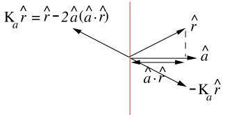
Figure 1: $K_{\hat{a}}{\hat{r}}$ is the reflection of ${\hat{r}}$ on the plane perpendicular to ${\hat{a}}$.

For any unit ${\mathbb{R}}^{3}$ vectors ${\hat{r}},{\hat{a}}$, define

$$K_{{\hat{a}}}{\hat{r}}={\hat{r}}-2{\hat{a}}({\hat{a}}\cdot{\hat{r}})\;.$$ (6)

From Fig.1, we see that $K_{{\hat{a}}}$ is a reflection: it reflects the vector ${\hat{r}}$ on the plane perpendicular to ${\hat{a}}$. Furthermore, $-K_{{\hat{a}}}$ is a pi rotation: it rotates the vector ${\hat{r}}$ by an angle of pi, about the axis ${\hat{a}}$. Note that

$$\sigma_{\hat{a}}\sigma_{\hat{r}}\sigma_{\hat{a}} = ({\hat{a}}\cdot{\hat{r}}+i\sigma_{{\hat{a}}\times{\hat{r}}})\sigma_{\hat{a}}$$ (7)

$$= ({\hat{a}}\cdot{\hat{r}})\sigma_{\hat{a}}-\sigma_{({\hat{a}}\times{\hat{r}})\times{\hat{a}}}$$ (8)

$$= ({\hat{a}}\cdot{\hat{r}})\sigma_{\hat{a}}-\sigma_{{\hat{r}}-{\hat{a}}({\hat{a}}\cdot{\hat{r}})}$$ (9)

$$= \sigma_{-K_{{\hat{a}}}{\hat{r}}}\;.$$ (10)

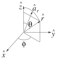
Figure 2: A pi rotation of ${\hat{z}}$ about ${\hat{a}}_{r}$ yields ${\hat{r}}$.

The eigenvectors of ${\sigma_{Z}}$ are given by

$${\sigma_{Z}}|\pm{\hat{z}}\rangle=(\pm 1)|\pm{\hat{z}}\rangle\;,$$ (11)

where

$$|+{\hat{z}}\rangle=\left[\begin{array}[]{c}1\\ 0\end{array}\right]=|0\rangle\;,\;\;|-{\hat{z}}\rangle=\left[\begin{array}[]{c}0\\ 1\end{array}\right]=|1\rangle\;.$$ (12)

It is also convenient to consider the eigenvectors of $\sigma_{\hat{r}}$, for any unit ${\mathbb{R}}^{3}$ vector ${\hat{r}}$. Given ${\hat{r}}$, we can always find a unit ${\mathbb{R}}^{3}$ vector ${\hat{a}}_{r}$ such that ${\hat{r}}$ is obtained by pi rotating ${\hat{z}}$ about ${\hat{a}}_{r}$. (See Fig.2). Eq.(11) implies that

$$(\sigma_{{\hat{a}}_{r}}\sigma_{\hat{z}}\sigma_{{\hat{a}}_{r}})\sigma_{{\hat{a}}_{r}}|0\rangle=\sigma_{{\hat{a}}_{r}}|0\rangle\;.$$ (13)

Furthermore,

$$\sigma_{\hat{r}}=\sigma_{{\hat{a}}_{r}}\sigma_{\hat{z}}\sigma_{{\hat{a}}_{r}}\;.$$ (14)

Hence, if we define $|{\hat{r}}\rangle$ by

$$|{\hat{r}}\rangle=\sigma_{{\hat{a}}_{r}}|0\rangle\;,$$ (15)

the Eq.(13) becomes

$$\sigma_{{\hat{r}}}|{\hat{r}}\rangle=|{\hat{r}}\rangle\;.$$ (16)

Eq.(16) itself implies that

$$\sigma_{{\hat{r}}}|\pm{\hat{r}}\rangle=\pm|\pm{\hat{r}}\rangle\;.$$ (17)

Thus, $|\pm{\hat{r}}\rangle$ defined by Eq.(15) are the eigenvectors of $\sigma_{\hat{r}}$ with eigenvalues $\pm 1$.

Given ${\hat{r}}$ in polar coordinates, we can express $|{\hat{r}}\rangle$ in terms of the polar coordinates of ${\hat{r}}$, as follows. Suppose

$${\hat{r}}=\left[\begin{array}[]{c}\sin\theta\cos\phi\\ \sin\theta\sin\phi\\ \cos\theta\end{array}\right]\;,$$ (18)

where $\theta\in[0,\frac{\pi}{2}]$ and $\phi\in[0,2\pi)$. Then, by definition, ${\hat{a}}_{r}$ has the same $\phi$ but half the $\theta$ coordinate:

$${\hat{a}}_{r}=\left[\begin{array}[]{c}\sin(\frac{\theta}{2})\cos\phi\\ \sin(\frac{\theta}{2})\sin\phi\\ \cos(\frac{\theta}{2})\end{array}\right]\;.$$ (19)

Thus,

$$|{\hat{r}}\rangle=\sigma_{{\hat{a}}_{r}}|0\rangle=\left[\begin{array}[]{c}{\hat{a}}_{z}\\ {\hat{a}}_{x}+i{\hat{a}}_{y}\end{array}\right]=\left[\begin{array}[]{c}\cos(\frac{\theta}{2})\\ e^{i\phi}\sin(\frac{\theta}{2})\end{array}\right]\;.$$ (20)

From Eq.(20), we get the following table.

$$\begin{array}[]{c|c}{\mathbb{R}}^{3}&{\mathbb{C}}^{2}\\ \hline\cr\pm{\hat{x}}&|\pm{\hat{x}}\rangle=\frac{1}{\sqrt{2}}\left[\begin{array}[]{c}1\\ \pm 1\end{array}\right]\\ \hline\cr\pm{\hat{y}}&|\pm{\hat{y}}\rangle=\frac{1}{\sqrt{2}}\left[\begin{array}[]{c}1\\ \pm i\end{array}\right]\\ \hline\cr{\hat{z}},-{\hat{z}}&|{\hat{z}}\rangle=\left[\begin{array}[]{c}1\\ 0\end{array}\right],|-{\hat{z}}\rangle=\left[\begin{array}[]{c}0\\ 1\end{array}\right]\end{array}\;$$ (21)

In general, the assignment ${\hat{r}}\mapsto|{\hat{r}}\rangle$ yields a map of ${\mathbb{R}}^{3}$ into ${\mathbb{C}}^{2}$, the 2-dimensional complex vector space spanned by complex linear combinations of $|0\rangle$ and $|1\rangle$. If we confine ourselves to the ${\hat{x}}-{\hat{z}}$ plane of ${\mathbb{R}}^{3}$, then that plane is mapped into the half-plane of all real linear combinations of $|0\rangle$ and $|1\rangle$ with non-negative $|0\rangle$ component. (Kets that differ by a phase factor or a normalization constant are equivalent).

Just like it is useful to consider the projection operators $|0\rangle\langle 0|$ and $|1\rangle\langle 1|$, it is also useful to consider the projection operator $|{\hat{r}}\rangle\langle{\hat{r}}|$. Recall the usual definitions of the number operator $n$ and its complement ${\overline{n}}$:

$$n=P_{1}=|1\rangle\langle 1|=\frac{1-{\sigma_{Z}}}{2}\;,$$ (22a)

$${\overline{n}}=1-n=P_{0}=|0\rangle\langle 0|=\frac{1+{\sigma_{Z}}}{2}\;.$$ (22b)

Rotating the coordinate system so that ${\hat{z}}$ goes to ${\hat{r}}$, we get

$$n_{\hat{r}}=P_{-{\hat{r}}}=|-{\hat{r}}\rangle\langle-{\hat{r}}|=\frac{1-\sigma_{\hat{r}}}{2}\;,$$ (23a)

$${\overline{n}}_{\hat{r}}=1-n_{\hat{r}}=P_{{\hat{r}}}=|{\hat{r}}\rangle\langle{\hat{r}}|=\frac{1+\sigma_{\hat{r}}}{2}\;.$$ (23b)

Note that if we define the reflection operator $K_{|{\hat{r}}\rangle}$ by

$$K_{|{\hat{r}}\rangle}=1-2|{\hat{r}}\rangle\langle{\hat{r}}|\;,$$ (24)

then

$$K_{|{\hat{r}}\rangle}=1-2{\overline{n}}_{\hat{r}}=(-1)^{{\overline{n}}_{\hat{r}}}=-\sigma_{\hat{r}}\;.$$ (25)

In general, the vectors in ${\mathbb{C}}^{2}$ are “packed twice as densely” as the corresponding vectors in ${\mathbb{R}}^{3}$. By this we mean that the angle between two vectors in ${\mathbb{C}}^{2}$ is always half the angle between the corresponding vectors in ${\mathbb{R}}^{3}$. To prove this, note that

$$|\langle{\hat{r}}_{1}|{\hat{r}}_{2}\rangle|^{2} = {\rm tr}(|{\hat{r}}_{1}\rangle\langle{\hat{r}}_{1}||{\hat{r}}_{2}\rangle\langle{\hat{r}}_{2}|)$$ (26)

$$= \frac{1}{4}{\rm tr}[(1+\sigma_{{\hat{r}}_{1}})(1+\sigma_{{\hat{r}}_{2}})]$$ (27)

$$= \frac{1}{4}{\rm tr}(1+\sigma_{{\hat{r}}_{1}}\sigma_{{\hat{r}}_{2}})$$ (28)

$$= \frac{1}{4}{\rm tr}(1+{\hat{r}}_{1}\cdot{\hat{r}}_{2})$$ (29)

$$= \frac{1}{2}(1+{\hat{r}}_{1}\cdot{\hat{r}}_{2})\;.$$ (30)

Thus, if ${\hat{r}}_{1}\cdot{\hat{r}}_{2}=\cos\alpha$, then $|\langle{\hat{r}}_{1}|{\hat{r}}_{2}\rangle|=\sqrt{\frac{1+\cos\alpha}{2}}=|\cos(\frac{\alpha}{2})|$.

Suppose $\theta\in{\mathbb{R}}$. A Taylor expansion easily establishes that

$$e^{i\theta{\sigma_{Z}}}=\cos\theta+i{\sigma_{Z}}\sin\theta\;.$$ (31)

Rotating the coordinate system so that ${\hat{z}}$ goes to ${\hat{r}}$, we get

$$e^{i\theta\sigma_{\hat{r}}}=\cos\theta+i\sigma_{\hat{r}}\sin\theta\;.$$ (32)

Suppose that ${\hat{a}}$ and ${\hat{b}}$ are two unit ${\mathbb{R}}^{3}$ vectors which make an angle $\theta$ between them. Let ${\hat{n}}=\frac{{\hat{a}}\times{\hat{b}}}{|{\hat{a}}\times{\hat{b}}|}$ be the unit ${\mathbb{R}}^{3}$ vector normal to the plane defined by ${\hat{a}}$ and ${\hat{b}}$. Then

$$\sigma_{\hat{a}}\sigma_{\hat{b}}={\hat{a}}\cdot{\hat{b}}+i\sigma_{{\hat{a}}\times{\hat{b}}}=\cos\theta+i\sigma_{\hat{n}}\sin\theta=e^{i\theta\sigma_{\hat{n}}}\;.$$ (33)

Thus, any SU(2) element $e^{i\theta\sigma_{\hat{n}}}$, where $\theta\in{\mathbb{R}}$ and ${\hat{n}}$ is a unit ${\mathbb{R}}^{3}$ vector, can be expressed (non-uniquely) as a product of two Paulions $\sigma_{\hat{a}}$ and $\sigma_{\hat{b}}$.

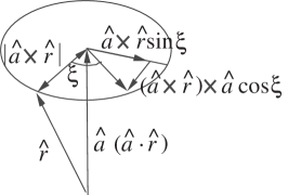
Figure 3: A finite rotation of ${\hat{r}}$ about axis ${\hat{a}}$ by an angle of $\xi$.

From Fig.3, it is clear that if $R_{{\hat{a}}}(\xi)$ is the rotation operator that rotates any unit ${\mathbb{R}}^{3}$ vector ${\hat{r}}$, by an angle $\xi\in{\mathbb{R}}$, about an axis defined by the unit ${\mathbb{R}}^{3}$ vector ${\hat{a}}$, then

$$R_{{\hat{a}}}(\xi){\hat{r}}={\hat{a}}({\hat{a}}\cdot{\hat{r}})+\sin(\xi){\hat{a}}\times{\hat{r}}+\cos(\xi)[{\hat{r}}-{\hat{a}}({\hat{a}}\cdot{\hat{r}})]\;.$$ (34)

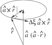
Figure 4: An infinitesimal rotation of ${\hat{r}}$ about axis ${\hat{a}}$ by an angle of $\Delta\xi$.

If ${\hat{r}},{\hat{a}}$ are unit ${\mathbb{R}}^{3}$ vectors and $\Delta\xi$ is an infinitesimal real number, then

$$e^{-i\frac{\Delta\xi}{2}\sigma_{\hat{a}}}\sigma_{\hat{r}}e^{i\frac{\Delta\xi}{2}\sigma_{\hat{a}}}\approx\sigma_{\hat{r}}-i\frac{\Delta\xi}{2}(\sigma_{\hat{a}}\sigma_{\hat{r}}-\sigma_{\hat{r}}\sigma_{\hat{a}})=\sigma_{{\hat{r}}+\Delta\xi({\hat{a}}\times{\hat{r}})}\;.$$ (35)

From Fig.4, ${\hat{r}}+\Delta\xi({\hat{a}}\times{\hat{r}})$ is just the vector ${\hat{r}}$ after an infinitesimal rotation $R_{{\hat{a}}}(\Delta\xi)$. By applying successively a large number of infinitesimal rotations $R_{{\hat{a}}}(\Delta\xi)$, we get a rotation $R_{{\hat{a}}}(\xi)$ over a finite angle $\xi\in{\mathbb{R}}$:

$$e^{-i\frac{\xi}{2}\sigma_{\hat{a}}}\sigma_{\hat{r}}e^{i\frac{\xi}{2}\sigma_{\hat{a}}}=\sigma_{R_{{\hat{a}}}(\xi){\hat{r}}}\ \;.$$ (36)

3 A SEO That Takes $|s^{\prime}\rangle$ to $|t\rangle$

In this section, we will explain a formalism and accompanying geometrical picture that can be used to describe both the original Grover’s algorithm, and the AFGA proposed in this paper.

Our goal is to find a SEO of SU(2) transformations that takes a starting state $|s^{\prime}\rangle\in{\mathbb{C}}^{2}$ to a target state $|t\rangle\in{\mathbb{C}}^{2}$. Without loss of generality, we will take

$$|t\rangle=|{\hat{z}}\rangle=|0\rangle\;$$ (37)

and

$$|s^{\prime}\rangle=|{\hat{s}}^{\prime}\rangle\mbox{ where }{\hat{s}}^{\prime}=(\sin\gamma){\hat{x}}+(\cos\gamma){\hat{z}}\;$$ (38)

with $\gamma\in[0,\pi]$.

Let $E_{j}$ for $j=0,1,\ldots,{j_{max}}$ denote

$$E_{j}=e^{-i\frac{\xi_{j}}{2}\sigma_{{\hat{a}}_{j}}}\;$$ (39)

where $\xi_{j}\in{\mathbb{R}}$ and the ${\hat{a}}_{j}$ are unit ${\mathbb{R}}^{3}$ vectors. Suppose ${\hat{s}}_{fin}$ is generated as follows

$${\hat{s}}_{fin}=[\prod_{j={j_{max}}\rightarrow 0}R_{{\hat{a}}_{j}}(\xi_{j})]{\hat{s}}^{\prime}\;.$$ (40)

(The arrow in the subscript of the product sign indicates the order in which to multiply the terms, this being an ordered product.) It follows that

$$\left|\langle 0|(\prod_{j={j_{max}}\rightarrow 0}E_{j})|s^{\prime}\rangle\right|^{2} = \langle 0|(\prod_{j={j_{max}}\rightarrow 0}E_{j})|s^{\prime}\rangle\langle s^{\prime}|(\prod_{j=0\rightarrow{j_{max}}}E^{\dagger}_{j})|0\rangle$$ (41)

$$= \langle 0|(\prod_{j={j_{max}}\rightarrow 0}E_{j})\left(\frac{1+\sigma_{{\hat{s}}^{\prime}}}{2}\right)(\prod_{j=0\rightarrow{j_{max}}}E^{\dagger}_{j})|0\rangle$$ (42)

$$= \frac{1}{2}\left(1+\langle 0|(\prod_{j={j_{max}}\rightarrow 0}e^{-i\frac{\xi_{j}}{2}\sigma_{{\hat{a}}_{j}}})\sigma_{{\hat{s}}^{\prime}}(\prod_{j=0\rightarrow{j_{max}}}e^{i\frac{\xi_{j}}{2}\sigma_{{\hat{a}}_{j}}})|0\rangle\right)$$ (43)

$$= \frac{1}{2}\left(1+\langle 0|\sigma_{{\hat{s}}_{fin}}|0\rangle\right)$$ (44)

$$= \frac{1}{2}\left(1+[{\hat{s}}_{fin}]_{z}\right)\;.$$ (45)

If we define $ERR$ by

$$ERR=1-\left|\langle 0|(\prod_{j={j_{max}}\rightarrow 0}E_{j})|s^{\prime}\rangle\right|^{2}\;,$$ (46)

then Eq.(45) implies that

$$ERR=\frac{1}{2}(1-[{\hat{s}}_{fin}]_{z})\;.$$ (47)

$ERR\geq 0$ is a measure of error. By Eq.(46), $ERR$ decreases towards zero as the SEO takes $|s^{\prime}\rangle$ closer to $|t\rangle$. Eq.(47) agrees with our expectation that $ERR$ goes to zero as the Z component of ${\hat{s}}_{fin}$ approaches one.

In the original Grover’s algorithm, $|s^{\prime}\rangle=U|s\rangle$, where $|s\rangle=|0\rangle^{\otimes{N_{B}}}$ and $U=H^{\otimes{N_{B}}}$. (Here $H$ denotes the one-bit Hadamard matrix $\frac{1}{\sqrt{2}}({\sigma_{X}}+{\sigma_{Z}})$. Also $|t\rangle=|t_{{N_{B}}-1}\rangle\otimes\ldots\otimes|t_{1}\rangle\otimes|t_{0}\rangle$ with $t_{i}=\delta_{i}^{i_{0}}$ for some $i_{0}\in\{0,1,\ldots,{N_{B}}-1\}$. Furthermore,

$$\prod_{j={j_{max}}\rightarrow 0}E_{j}=G^{N_{steps}}\;,$$ (48)

where $N_{steps}$ is the number of steps (i.e., queries) and

$$G = -(-1)^{|s^{\prime}\rangle\langle s^{\prime}|}(-1)^{|t\rangle\langle t|}$$ (49)

$$= e^{i\pi}e^{i\pi{\overline{n}}_{{\hat{s}}^{\prime}}}e^{i\pi{\overline{n}}_{{\hat{z}}}}$$ (50)

$$= e^{i\frac{\pi}{2}\sigma_{{\hat{s}}^{\prime}}}e^{i\frac{\pi}{2}{\sigma_{Z}}}\;.$$ (51)

Note that $G$ corresponds to a small rotation about the ${\hat{y}}$ axis. Indeed,

$$G = -(-1)^{{\overline{n}}_{{\hat{s}}^{\prime}}}(-1)^{{\overline{n}}_{\hat{z}}}$$ (52)

$$= -\sigma_{{\hat{s}}^{\prime}}{\sigma_{Z}}$$ (53)

$$= -({\hat{s}}^{\prime}\cdot{\hat{z}}+i\sigma_{{\hat{s}}^{\prime}\times{\hat{z}}})$$ (54)

$$= -(\cos\gamma-i{\sigma_{Y}}\sin\gamma)$$ (55)

$$= e^{i(\pi-\gamma){\sigma_{Y}}}=e^{i\frac{\Delta\gamma}{2}{\sigma_{Y}}}\;$$ (56)

where $\Delta\gamma=2(\pi-\gamma)\geq 0$. Thus

$$R_{{\hat{s}}^{\prime}}(-\pi)R_{{\hat{z}}}(-\pi)=R_{{\hat{y}}}(-\Delta\gamma)\;.$$ (57)

From $\cos(\frac{\gamma}{2})=\langle s^{\prime}|t\rangle=\frac{1}{\sqrt{{N_{S}}}}$, it follows that $\Delta\gamma={\cal O}(\frac{1}{\sqrt{{N_{S}}}})$.

Note also that $G$ can be p-compiled trivially. Indeed, if $P_{0}$ and $P_{1}$ are defined as in Eqs.(22),

$$(-1)^{|t\rangle\langle t|}=(-1)^{\prod_{\beta=0}^{{N_{B}}-1}P_{t_{i}}(\beta)}\;,$$ (58a)

and

$$(-1)^{|s^{\prime}\rangle\langle s^{\prime}|}=H^{\otimes{N_{B}}}\left[(-1)^{|0^{N_{B}}\rangle\langle 0^{N_{B}}|}\right]H^{\otimes{N_{B}}}=H^{\otimes{N_{B}}}\left[(-1)^{\prod_{\beta=0}^{{N_{B}}-1}P_{0}(\beta)}\right]H^{\otimes{N_{B}}}\;.$$ (58b)

Next, let’s describe our AFGA. We take

$$\prod_{j={j_{max}}\rightarrow 0}E_{j} = \prod_{j=\infty\rightarrow 0}(e^{i\alpha_{j}|s^{\prime}\rangle\langle s^{\prime}|}e^{i\Delta\lambda|t\rangle\langle t|})$$ (59)

$$= \prod_{j=\infty\rightarrow 0}(e^{\frac{i}{2}(\alpha_{j}+\Delta\lambda)}e^{i\frac{\alpha_{j}}{2}\sigma_{{\hat{s}}^{\prime}}}e^{i\frac{\Delta\lambda}{2}{\sigma_{Z}}})\;,$$ (60)

for some $\Delta{\lambda}\in[0,\pi]$ and some infinite sequence of $\alpha_{j}\in{\mathbb{R}}$. In the original Grover’s algorithm, $\Delta{\lambda}$ and all the $\alpha_{j}$ are fixed at $\pi$. That’s why we say our algorithm is adaptive. We will also assume that

$$R_{{\hat{s}}^{\prime}}(-\alpha_{j})R_{{\hat{z}}}(-\Delta\lambda)=R_{\hat{y}}(-\bar{\Delta}\gamma_{j})\;$$ (61)

for some $\bar{\Delta}\gamma_{j}\in{\mathbb{R}}$, and that we know how to p-compile $e^{i\alpha_{j}|s^{\prime}\rangle\langle s^{\prime}|}$ and $e^{i\Delta\lambda|t\rangle\langle t|}$. If $|s^{\prime}\rangle$ and $|t\rangle$ are the same as in the original Grover’s algorithm, then we do indeed know how to p-compile these operators. (Just replace the $(-1)=e^{i\pi}$ phase factors in Eqs.(58) by $e^{i\alpha_{j}}$ and $e^{i\Delta\lambda}$.)

Our AFGA has a total of two input parameters: $\Delta{\lambda}\in[0,\pi]$ (the angle of each consecutive ${\hat{z}}$ rotation), and $\gamma\in[0,\pi]$ (the angle which ${\hat{s}}^{\prime}$ makes with ${\hat{z}}$). For the AFGA to be fully specified, we still need to specify, as a function of these two input parameters, a suitable sequence of $\alpha_{j}$ that makes $ERR$ converge to zero. We will do this in the next section.

4 Bouncing Between Two Longitudes

In this section, we give a suitable sequence $\{\alpha_{j}\}_{j=0}^{\infty}$ for our AFGA, as a function of the two input parameters $\Delta{\lambda}$ and $\gamma$. We will do this guided by the geometrical picture of bouncing between two great circles of longitude of the unit sphere.

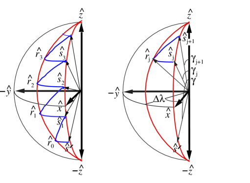
Figure 5: Unit ${\mathbb{R}}^{3}$ vectors and angles used in our AFGA. Note how we “bounce between two longitudes”.

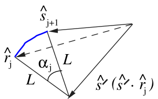
Figure 6: Geometry defining angle $\alpha_{j}$ and radius $L$.

It is convenient to define two sequences of unit ${\mathbb{R}}^{3}$ vectors $\{{\hat{s}}_{j}\}_{j=0}^{\infty}$, and $\{{\hat{r}}_{j}\}_{j=0}^{\infty}$ by the recursion relation:

$${\hat{s}}_{0}={\hat{s}}^{\prime}\;$$ (62)

$$\begin{array}[]{l}{\hat{r}}_{j}=R_{\hat{z}}(-\Delta{\lambda}){\hat{s}}_{j},\\ {\hat{s}}_{j+1}=R_{{\hat{s}}^{\prime}}(-\alpha_{j}){\hat{r}}_{j}\\ {\hat{s}}_{j+1}=R_{\hat{y}}(-\bar{\Delta}\gamma_{j}){\hat{s}}_{j}\end{array}\;$$ (63)

for $j=0,1,\ldots$. According to Eqs.(63),

$$\begin{array}[]{l}\angle({\hat{r}}_{j},{\hat{s}}_{j})=\Delta{\lambda},\\ \angle({\hat{s}}_{j+1},{\hat{r}}_{j})=\alpha_{j},\\ \angle({\hat{s}}_{j+1},{\hat{s}}_{j})=\bar{\Delta}\gamma_{j}\end{array}\;.$$ (64)

See Figs.5 for a geometrical picture of the ${\hat{s}}_{j}$ and ${\hat{r}}_{j}$ sequences of vectors. The arrowheads of all the ${\hat{s}}_{j}$ vectors lie on the great circle of longitude located at the intersection of the ${\hat{x}}-{\hat{z}}$ plane and the unit sphere. The arrowheads of all the ${\hat{r}}_{j}$ vectors lie on the great circle of longitude which makes an angle of $\Delta{\lambda}$ with the ${\hat{s}}_{j}$ great circle of longitude.

The angles $\gamma_{j}$ and $\bar{\Delta}\gamma_{j}$ are defined in terms of the vectors ${\hat{s}}_{j}$ as follows:

$$\angle({\hat{s}}^{\prime},{\hat{z}})=\gamma=\gamma_{0}\;$$ (65)

and

$$\angle({\hat{s}}_{j},{\hat{z}})=\gamma_{j}\;,\;\;\angle({\hat{s}}_{j+1},{\hat{z}})=\gamma_{j+1}\;\;\bar{\Delta}\gamma_{j}=-\Delta\gamma_{j}=\gamma_{j}-\gamma_{j+1}\;$$ (66)

for $j=0,1,\ldots$.

Note from Fig.5 and 6 that

$$\angle({\hat{r}}_{j},{\hat{s}}^{\prime})=\angle({\hat{s}}_{j+1},{\hat{s}}^{\prime})=\gamma-\gamma_{j+1}=\gamma-\gamma_{j}+\bar{\Delta}\gamma_{j}\;.$$ (67)

Since

$${\hat{r}}_{j} = R_{\hat{z}}(-\Delta{\lambda}){\hat{s}}_{j}$$ (68)

$$= {\hat{z}}({\hat{z}}\cdot{\hat{s}}_{j})-{\hat{z}}\times{\hat{s}}_{j}S_{\Delta{\lambda}}+[{\hat{s}}_{j}-({\hat{s}}_{j}\cdot{\hat{z}}){\hat{z}}]C_{\Delta{\lambda}}$$ (69)

$$= {\hat{z}}C_{\gamma_{j}}(1-C_{\Delta{\lambda}})-{\hat{y}}S_{\gamma_{j}}S_{\Delta{\lambda}}+{\hat{s}}_{j}C_{\Delta{\lambda}}\;,$$ (70)

it follows that

$${\hat{r}}_{j}\cdot{\hat{s}}^{\prime} = C_{\gamma}C_{\gamma_{j}}(1-C_{\Delta{\lambda}})+\cos(\gamma-\gamma_{j})C_{\Delta{\lambda}}$$ (71)

$$= C_{\gamma}C_{\gamma_{j}}+S_{\gamma}S_{\gamma_{j}}C_{\Delta{\lambda}}\;.$$ (72)

As is usual in the C programming language, define $\theta={\rm atan}2(y,x)$ only if $\tan\theta=y/x$.(Think of the comma in ${\rm atan}2(y,x)$ as a slash indicating division). Eq.(67) implies that

$$\gamma-\gamma_{j}+\bar{\Delta}\gamma_{j}={{\rm atan}2}(\pm\sqrt{1-({\hat{r}}_{j}\cdot{\hat{s}}^{\prime})^{2}},{\hat{r}}_{j}\cdot{\hat{s}}^{\prime})\;.$$ (73)

Assume $\angle({\hat{r}}_{j},{\hat{s}}^{\prime})\in[0,\pi]$. This means we choose the solution with the positive sign in Eq.(73).

To summarize, we’ve shown that

$$\bar{\Delta}\gamma_{j}=-\gamma+\gamma_{j}+{{\rm atan}2}(\sqrt{1-({\hat{r}}_{j}\cdot{\hat{s}}^{\prime})^{2}},{\hat{r}}_{j}\cdot{\hat{s}}^{\prime})\;$$ (74a) where

$${\hat{r}}_{j}\cdot{\hat{s}}^{\prime}=C_{\gamma}C_{\gamma_{j}}+S_{\gamma}S_{\gamma_{j}}C_{\Delta{\lambda}}\;$$ (74b) Eqs.(74) and $\gamma_{0}=\gamma$ allows us to find the sequence $\{\gamma_{j}\}_{j=0}^{\infty}$. The sequence $\{\gamma_{j}\}_{j=0}^{\infty}$ and ${\hat{s}}_{0}={\hat{s}}^{\prime}$ allows us to find the sequence $\{{\hat{s}}_{j}\}_{j=0}^{\infty}$.

Next we solve for the sequence $\{\alpha_{j}\}_{j=0}^{\infty}$, assuming that we know the two input parameters $\Delta{\lambda}$ and $\gamma$, and the sequence $\{\gamma_{j}\}_{j=0}^{\infty}$. We can find $\alpha_{j}$ by considering Fig.6. That figure defines $L$ as

$$L=|{\hat{r}}_{j}-{\hat{s}}^{\prime}({\hat{s}}^{\prime}\cdot{\hat{r}}_{j})|=\sqrt{1-({\hat{r}}_{j}\cdot{\hat{s}}^{\prime})^{2}}=|\sin(\gamma-\gamma_{j}+\bar{\Delta}\gamma_{j})|=\sin(\gamma-\gamma_{j}+\bar{\Delta}\gamma_{j})\;.$$ (75)

Note also that

$${\hat{s}}_{j+1}=R_{{\hat{y}}}(-\bar{\Delta}\gamma_{j}){\hat{s}}_{j}=-{\hat{y}}\times{\hat{s}}_{j}S_{\bar{\Delta}\gamma_{j}}+{\hat{s}}_{j}C_{\bar{\Delta}\gamma_{j}}\;.$$ (76)

It follows from Fig.6 that

$$L^{2}\sin\alpha_{j} = [{\hat{r}}_{j}-{\hat{s}}^{\prime}({\hat{s}}^{\prime}\cdot{\hat{r}}_{j})]\times[{\hat{s}}_{j+1}-{\hat{s}}^{\prime}({\hat{s}}^{\prime}\cdot{\hat{r}}_{j})]\cdot(-{\hat{s}}^{\prime})$$ (77)

$$= {\hat{r}}_{j}\times{\hat{s}}_{j+1}\cdot(-{\hat{s}}^{\prime})$$ (78)

$$= S_{\bar{\Delta}\gamma_{j}}[{\hat{r}}_{j}\times({\hat{y}}\times{\hat{s}}_{j})\cdot{\hat{s}}^{\prime}]+C_{\bar{\Delta}\gamma_{j}}[-{\hat{r}}_{j}\times{\hat{s}}_{j}\cdot{\hat{s}}^{\prime}]\;.$$ (79)

But by virtue of Eq.(70) for ${\hat{r}}_{j}$,

$${\hat{r}}_{j}\times({\hat{y}}\times{\hat{s}}_{j})\cdot{\hat{s}}^{\prime}=-({\hat{s}}_{j}\cdot{\hat{s}}^{\prime})({\hat{r}}_{j}\cdot{\hat{y}})=\cos(\gamma-\gamma_{j})S_{\gamma_{j}}S_{\Delta{\lambda}}\;,$$ (80)

and

$${\hat{r}}_{j}\times{\hat{s}}_{j}\cdot{\hat{s}}^{\prime}=-({\hat{y}}\times{\hat{s}}_{j}\cdot{\hat{s}}^{\prime})S_{\gamma_{j}}S_{\Delta{\lambda}}=-\sin(\gamma-\gamma_{j})S_{\gamma_{j}}S_{\Delta{\lambda}}\;$$ (81)

so

$$L^{2}\sin\alpha_{j}=\sin(\gamma-\gamma_{j}+\bar{\Delta}\gamma_{j})S_{\gamma_{j}}S_{\Delta{\lambda}}\;.$$ (82)

It also follows from Fig.6 that

$$L^{2}\cos\alpha_{j} = [{\hat{r}}_{j}-{\hat{s}}^{\prime}({\hat{s}}^{\prime}\cdot{\hat{r}}_{j})]\cdot[{\hat{s}}_{j+1}-{\hat{s}}^{\prime}({\hat{s}}^{\prime}\cdot{\hat{r}}_{j})]$$ (83)

$$= [{\hat{r}}_{j}-{\hat{s}}^{\prime}({\hat{s}}^{\prime}\cdot{\hat{r}}_{j})]\cdot{\hat{s}}_{j+1}$$ (84)

$$= [{\hat{r}}_{j}-{\hat{s}}^{\prime}({\hat{s}}^{\prime}\cdot{\hat{r}}_{j})]\cdot[-{\hat{y}}\times{\hat{s}}_{j}S_{\bar{\Delta}\gamma_{j}}+{\hat{s}}_{j}C_{\bar{\Delta}\gamma_{j}}]$$ (85)

$$= \left\{\begin{array}[]{l}S_{\bar{\Delta}\gamma_{j}}[{\hat{r}}_{j}\times{\hat{s}}_{j}\cdot{\hat{y}}+\sin(\gamma-\gamma_{j}){\hat{r}}_{j}\cdot{\hat{s}}^{\prime}]\\ +C_{\bar{\Delta}\gamma_{j}}[{\hat{r}}_{j}\cdot{\hat{s}}_{j}-\cos(\gamma-\gamma_{j}){\hat{r}}_{j}\cdot{\hat{s}}^{\prime}]\end{array}\right.\;.$$ (88)

But by virtue of Eq.(70) for ${\hat{r}}_{j}$,

$${\hat{r}}_{j}\times{\hat{s}}_{j}\cdot{\hat{y}}=({\hat{z}}\times{\hat{s}}_{j}\cdot{\hat{y}})C_{\gamma_{j}}(1-C_{\Delta{\lambda}})=S_{\gamma_{j}}C_{\gamma_{j}}(1-C_{\Delta{\lambda}})\;,$$ (89)

and

$${\hat{r}}_{j}\cdot{\hat{s}}_{j}=C^{2}_{\gamma_{j}}(1-C_{\Delta{\lambda}})+C_{\Delta{\lambda}}=C^{2}_{\gamma_{j}}+S^{2}_{\gamma_{j}}C_{\Delta{\lambda}}\;$$ (90)

so

$$L^{2}\cos\alpha_{j}=\left\{\begin{array}[]{l}S_{\bar{\Delta}\gamma_{j}}[C_{\gamma_{j}}S_{\gamma_{j}}(1-C_{\Delta{\lambda}})+\sin(\gamma-\gamma_{j}){\hat{r}}_{j}\cdot{\hat{s}}^{\prime}]\\ +C_{\bar{\Delta}\gamma_{j}}[C^{2}_{\gamma_{j}}+S^{2}_{\gamma_{j}}C_{\Delta{\lambda}}-\cos(\gamma-\gamma_{j}){\hat{r}}_{j}\cdot{\hat{s}}^{\prime}]\end{array}\right.\;.$$ (91)

To summarize,

$$\alpha_{j}={\rm atan}2(L^{2}\sin\alpha_{j},L^{2}\cos\alpha_{j})\;,$$ (92) where $L^{2}\sin\alpha_{j}$ and $L^{2}\cos\alpha_{j}$ are given by Eqs.(82) and (91).

5 Software and Numerical Results

In this section, we describe some simple software that calculates, among other things, the phases $\alpha_{j}$ used in our AFGA. We also present and discuss some examples of the output of the software.

gamma(degs) = 1.7315e+02
del_lam(degs) = 1.3500e+02
num_steps = 20
j   gam_j(degs) alp_j(degs) vr_x        vr_y        vr_z        vs_x        vs_y        vs_z
0   1.7315e+02  1.5735e+02  -8.4337e-02 -8.4337e-02 -9.9286e-01 1.1927e-01  0.0000e+00  -9.9286e-01
1   1.6050e+02  1.4576e+02  -2.3607e-01 -2.3607e-01 -9.4263e-01 3.3385e-01  -2.7756e-17 -9.4263e-01
2   1.4835e+02  1.4171e+02  -3.7109e-01 -3.7109e-01 -8.5122e-01 5.2480e-01  -1.1102e-16 -8.5122e-01
3   1.3636e+02  1.3947e+02  -4.8795e-01 -4.8795e-01 -7.2375e-01 6.9006e-01  -1.6653e-16 -7.2375e-01
4   1.2448e+02  1.3795e+02  -5.8289e-01 -5.8289e-01 -5.6611e-01 8.2433e-01  -2.2204e-16 -5.6611e-01
5   1.1266e+02  1.3676e+02  -6.5253e-01 -6.5253e-01 -3.8523e-01 9.2282e-01  -1.1102e-16 -3.8523e-01
6   1.0089e+02  1.3572e+02  -6.9438e-01 -6.9438e-01 -1.8888e-01 9.8200e-01  5.5511e-17  -1.8888e-01
7   8.9160e+01  1.3472e+02  -7.0703e-01 -7.0703e-01 1.4652e-02  9.9989e-01  1.6653e-16  1.4652e-02
8   7.7476e+01  1.3369e+02  -6.9028e-01 -6.9028e-01 2.1686e-01  9.7620e-01  -5.5511e-17 2.1686e-01
9   6.5834e+01  1.3253e+02  -6.4514e-01 -6.4514e-01 4.0938e-01  9.1236e-01  -2.2204e-16 4.0938e-01
10  5.4242e+01  1.3107e+02  -5.7381e-01 -5.7381e-01 5.8436e-01  8.1149e-01  0.0000e+00  5.8436e-01
11  4.2712e+01  1.2901e+02  -4.7964e-01 -4.7964e-01 7.3478e-01  6.7831e-01  -2.2204e-16 7.3478e-01
12  3.1268e+01  1.2557e+02  -3.6702e-01 -3.6702e-01 8.5475e-01  5.1905e-01  -1.6653e-16 8.5475e-01
13  1.9971e+01  1.1787e+02  -2.4151e-01 -2.4151e-01 9.3986e-01  3.4155e-01  -3.3307e-16 9.3986e-01
14  9.0040e+00  8.5904e+01  -1.1067e-01 -1.1067e-01 9.8768e-01  1.5650e-01  1.9429e-16  9.8768e-01
15  -4.8000e-01 -2.7100e+00 5.9237e-03  5.9237e-03  9.9996e-01  -8.3774e-03 7.5114e-16  9.9996e-01
16  3.4738e-01  2.1347e+00  -4.2871e-03 -4.2871e-03 9.9998e-01  6.0629e-03  -7.6762e-16 9.9998e-01
17  -2.4109e-01 -1.3945e+00 2.9753e-03  2.9753e-03  9.9999e-01  -4.2078e-03 4.4149e-16  9.9999e-01
18  1.7254e-01  1.0412e+00  -2.1293e-03 -2.1293e-03 1.0000e+00  3.0113e-03  5.0394e-16  1.0000e+00
19  -1.2090e-01 -7.0794e-01 1.4921e-03  1.4921e-03  1.0000e+00  -2.1101e-03 -1.6948e-15 1.0000e+00
20  8.6014e-02  5.1447e-01  -1.0615e-03 -1.0615e-03 1.0000e+00  1.5012e-03  1.1501e-15  1.0000e+00

Figure 7: Typical output produced by running afga.m.

We’ve written 3 Octave/Matlab m-files called afga.m, afga_step.m and afga_rot.m that implement some of the results of this paper. The main file afga.m calls functions in afga_step.m and afga_rot.m.

The first 3 lines of afga.m instantiate the 3 input parameters g0_degs (=$\gamma$ in degrees), del_lam_degs($=\Delta{\lambda}$ in degrees), and num_steps (= maximum value of $j$ that will be considered. $j$ will range from 0 to num_steps)

Each time afga.m runs successfully, it outputs a text file called afga.txt. Fig.7 illustrates a typical afga.txt file. The first 3 lines record the inputs. The next line labels the columns of the file. The column labels are

• j = $j$

• gam_j(degs) = $\gamma_{j}$ in degrees

• alp_j(degs) = $\alpha_{j}$ in degrees

• vr_x = $[{\hat{r}}_{j}]_{x}$

• vr_y = $[{\hat{r}}_{j}]_{y}$

• vr_z = $[{\hat{r}}_{j}]_{z}$

• vs_x = $[{\hat{s}}_{j}]_{x}$

• vs_y = $[{\hat{s}}_{j}]_{y}$

• vs_z = $[{\hat{s}}_{j}]_{z}$

Following the line of column labels are num_steps+1 lines of output data.

In afga.txt, data in each line is separated by a tab. Thus, the full afga.txt file can be cut-and-pasted into an Excel spreadsheet or other plotting software in order to plot it.

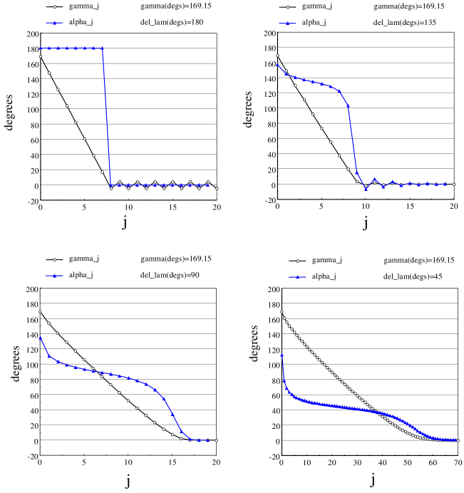
Figure 8: Values of $\gamma_{j}$ and $\alpha_{j}$ obtained with afga.m for $\gamma=169.15^{0}$ and various values of $\Delta{\lambda}$

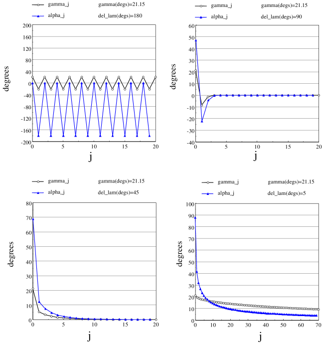
Figure 9: Values of $\gamma_{j}$ and $\alpha_{j}$ obtained with afga.m for $\gamma=21.15^{0}$ and various values of $\Delta{\lambda}$

Fig.8 shows the values of $\gamma_{j}$ and $\alpha_{j}$ obtained with afga.m for $\gamma=169.15^{0}$ and various values of $\Delta{\lambda}$. Fig.9 shows the same thing but for $\gamma=21.15^{0}$. We see that $\gamma_{j}$ decreases almost linearly from $\gamma$ to near zero. The behavior of $\gamma_{j}$ near zero depends on the value of $\Delta{\lambda}$. For $0\leq\Delta{\lambda}<\pi$, $\gamma_{j}$ goes to zero without too many oscillations. For $\Delta{\lambda}$ precisely equal to $\pi$, $\gamma_{j}$ never converges to zero. It gets trapped near zero, oscillating about it with a constant amplitude.

In Appendix A, we discuss in more detail the behavior of our AFGA when $\Delta{\lambda}=\pi$. This case most closely resembles the original Grover’s algorithm.

In Appendix B, we discuss the continuum limit where $\bar{\Delta}\gamma_{j}$ tends to zero for all $j$. This limit is a smoothed out version of the discrete case. It is easily solved, and gives a good idea of the rate of convergence of $\gamma_{j}$ (and of $ERR$) towards zero (when $\Delta{\lambda}\neq\pi$) as $j$ tends to infinity.

Appendix A Appendix: When $\Delta{\lambda}=\pi$

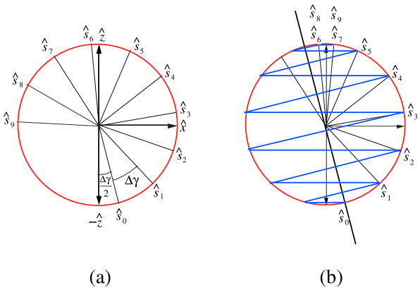
Figure 10: (a)${\hat{s}}_{j}$ vectors for original Grover’s algorithm. (b)${\hat{s}}_{j}$ vectors for our AFGA with $\Delta{\lambda}=\pi$ and the same $\gamma$ as in (a).

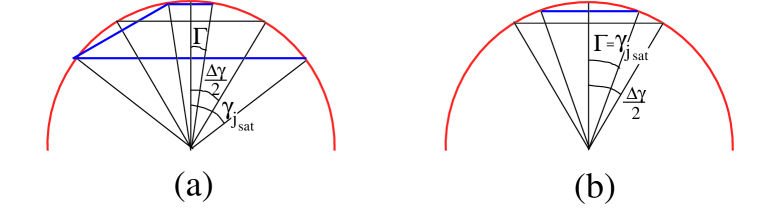
Figure 11: (a)$\Gamma$ when $\gamma_{{j_{sat}}}>\frac{\Delta\gamma}{2}$. (b)$\Gamma$ when $\gamma_{{j_{sat}}}<\frac{\Delta\gamma}{2}$.

In this section, we discuss the $\Delta{\lambda}=\pi$ case of our AFGA.

Fig.10(a) shows the pattern of the ${\hat{s}}_{j}$ vectors for the original Grover’s algorithm, and Fig.10(b) shows the pattern for our AFGA with $\Delta{\lambda}=\pi$ and the same $\gamma$ as in (a). There is a critical $j$, call it ${j_{sat}}$ (“sat” for saturation). (a) and (b) have the same ${\hat{s}}_{j}$ vectors for $j=0,1,\ldots,{j_{sat}}$. For $j>{j_{sat}}$, the ${\hat{s}}_{j}$ vectors of (a) continue to decrease their angle (with respect to ${\hat{z}}$) at a uniform rate, past the North Pole, whereas the ${\hat{s}}_{j}$ vectors of (b) get trapped in the neighborhood of the North Pole, bouncing back and forth, making an angle of $\pm\Gamma$ with respect to ${\hat{z}}$. In other words, the pattern observed is like this:

$$\begin{array}[]{c|c|c}j&\gamma_{j}\mbox{ for }(a)&\gamma_{j}\mbox{ for }(b)\\ \hline\cr\hline\cr\vdots&\vdots&\vdots\\ \hline\cr{j_{sat}}-1&\gamma_{{j_{sat}}}+\Delta\gamma&\gamma_{{j_{sat}}}+\Delta\gamma\\ \hline\cr{j_{sat}}&\gamma_{{j_{sat}}}&\gamma_{{j_{sat}}}\\ \hline\cr{j_{sat}}+1&\gamma_{{j_{sat}}}-\Delta\gamma&-\Gamma\\ \hline\cr{j_{sat}}+2&\gamma_{{j_{sat}}}-2\Delta\gamma&\Gamma\\ \hline\cr{j_{sat}}+3&\gamma_{{j_{sat}}}-3\Delta\gamma&-\Gamma\\ \hline\cr{j_{sat}}+3&\gamma_{{j_{sat}}}-4\Delta\gamma&\Gamma\\ \hline\cr\vdots&\vdots&\vdots\\ \hline\cr\end{array};.$$ (93)

${j_{sat}}$ is defined by the constraints that $\gamma_{{j_{sat}}-1}>\Delta\gamma$ and $0\leq\gamma_{{j_{sat}}}<\Delta\gamma$.

As shown by Fig.11,

$$\Gamma = \left\{\begin{array}[]{ll}\gamma_{j_{sat}}&\mbox{ if }0\leq\gamma_{j_{sat}}\leq\frac{\Delta\gamma}{2}\\ \Delta\gamma-\gamma_{j_{sat}}&\mbox{ if }\frac{\Delta\gamma}{2}\leq\gamma_{j_{sat}}\leq\Delta\gamma\end{array}\right.$$ (96)

$$= \min(\gamma_{j_{sat}},\Delta\gamma-\gamma_{j_{sat}})\;.$$ (97)

For example,

$$\begin{array}[]{r||r|r|r}\gamma\mbox{(degs)}&\Delta\gamma\mbox{(degs)}&\gamma_{j_{sat}}\mbox{(degs)}&\Gamma\mbox{(degs)}\\ \hline\cr\hline\cr 160&2(20)&0&0\\ \hline\cr 164&2(16)&4&4\\ \hline\cr 166&2(14)&26&2\\ \hline\cr\end{array}\;.$$ (98)

The last column of Eq.(98) was calculated using Eq.(97) and then checked using afga.m.

Appendix B Appendix: Continuum Limit

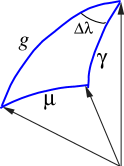
Figure 12: A spherical triangle with sides of length $\mu$, $\gamma$ and $g$, and angle $\Delta{\lambda}$ between the $g$ and $\gamma$ sides. The spherical triangle has sides which are segments of great circles of the unit sphere.

In this section, we explore $\gamma_{j}$ in the continuum limit.

Suppose we take the limit where $\bar{\Delta}\gamma_{j}$ tends to zero for all $j\geq 0$. We replace $j$ by a real number $t\geq 0$ and $\gamma_{j}$ by a continuous function $g(t)$ of $t$. $\bar{\Delta}\gamma_{j}=\gamma_{j}-\gamma_{j+1}\rightarrow-\frac{dg}{dt}$ and Eq.(74) tends to

$$-\frac{dg}{dt}=-\gamma+g+{\rm atan}2(|S_{\mu(g)}|,C_{\mu(g)})\;,$$ (99)

where $\mu(g)$ satisfies

$$C_{\mu(g)}=C_{\gamma}C_{g}+S_{\gamma}S_{g}C_{\Delta{\lambda}}\;.$$ (100)

Henceforth, we will restrict our attention to the case $0\leq g\leq\gamma\leq\pi$.

In general, note that if $\cos(\alpha)=\cos(\beta)$, then $\alpha=\pm\beta+2\pi N$ for some integer $N$. Hence, Eq.(100) doesn’t specify $\mu(g)$ uniquely. However, the “Law of Cosines” of spherical trigonometry tells us that one possible value for $\mu(g)$ is the length of the side of the spherical triangle portrayed in Fig.12. Henceforth, we will identify $\mu(g)$ with this unique geometrical value. When $\mu$ is given this geometrical value, since $0\leq g\leq\gamma\leq\pi$, $\mu\in[0,2\pi]$. Since ${\rm atan}2(|S_{\mu}|,C_{\mu})\in[0,\pi]$, we must have

$${\rm atan}2(|S_{\mu}|,C_{\mu}) = \left\{\begin{array}[]{ll}\mu&\mbox{ if }\mu\in[0,\pi]\\ 2\pi-\mu&\mbox{ if }\mu\in[\pi,2\pi]\end{array}\right.$$ (103)

$$= \min(\mu,2\pi-\mu)\;.$$ (104)

Hence, when $\mu(g)$ is given its geometrical value,

$$-\frac{dg}{dt}=-\gamma+g+\min(\mu,2\pi-\mu)\;.$$ (105)

Eq.(105) can be solved in closed form in some special cases:

1. $|g|<<1$: In this case, we get from Eq.(100),

   $$C_{\mu}\approx C_{\gamma}+S_{\gamma}gC_{\Delta{\lambda}}\approx\cos(\gamma-gC_{\Delta{\lambda}})\;.$$ (106)

   so $\mu\approx\gamma-gC_{\Delta{\lambda}}$. Hence,

   $$-\frac{dg}{dt}\approx g(1-C_{\Delta{\lambda}})\;\;\;\;\Rightarrow g\approx(const.)e^{-t(1-C_{\Delta{\lambda}})}\;.$$ (107)

2. $0\leq\gamma-g<<1$: In this case,

   $$-\frac{dg}{dt}\approx\min[\mu(\gamma),2\pi-\mu(\gamma)]\;\;\;\;\Rightarrow g\approx\gamma-t\min[\mu(\gamma),2\pi-\mu(\gamma)]\;$$ (108)

   1. $\Delta{\lambda}=\pi$: In this case, we see from Fig.12 that $\mu(\gamma)=2\gamma$. Hence

      $$g\approx\left\{\begin{array}[]{ll}\gamma-t2(\pi-\gamma)=\gamma-t\Delta\gamma&\mbox{if }\;\gamma>\frac{\pi}{2}\\ \gamma-t2\gamma&\mbox{if }\;\gamma<\frac{\pi}{2}\end{array}\right.\;.$$ (109)

   2. $0\leq\Delta{\lambda}<<1$: In this case, by virtue of Eq.(100),

      $$C_{\mu}\approx C_{\gamma}^{2}+S_{\gamma}^{2}C_{\Delta{\lambda}}\approx 1-\frac{1}{2}S_{\gamma}^{2}(\Delta{\lambda})^{2}\approx\cos(S_{\gamma}\Delta{\lambda})\;,$$ (110)

      so $\mu(\gamma)\approx S_{\gamma}\Delta{\lambda}$. Hence

      $$g\approx\gamma-tS_{\gamma}\Delta{\lambda}\;.$$ (111)

And what is the maximum $|dg/dt|$ for $g\approx\gamma$? When $g\approx\gamma$,

$$\max_{\Delta{\lambda}\in[0,\pi]}|dg/dt|=|dg/dt|_{\Delta{\lambda}=\pi}=\min[2\gamma,2\pi-2\gamma]\;.$$ (112)