Wright–Fisher diffusion with negative mutation rates

Abstract

We study a family of $n$-dimensional diffusions, taking values in the unit simplex of vectors with nonnegative coordinates that add up to one. These processes satisfy stochastic differential equations which are similar to the ones for the classical Wright–Fisher diffusions, except that the “mutation rates” are now nonpositive. This model, suggested by Aldous, appears in the study of a conjectured diffusion limit for a Markov chain on Cladograms. The striking feature of these models is that the boundary is not reflecting, and we kill the process once it hits the boundary. We derive the explicit exit distribution from the simplex and probabilistic bounds on the exit time. We also prove that these processes can be viewed as a “stochastic time-reversal” of a Wright–Fisher process of increasing dimensions and conditioned at a random time. A key idea in our proofs is a skew-product construction using certain one-dimensional diffusions called Bessel-square processes of negative dimensions, which have been recently introduced by Göing-Jaeschke and Yor.

1 Introduction

An $n$-leaf Cladogram is an unrooted tree with $n\geq 4$ labeled leaves (vertices with degree one) and $(n-2)$ other unlabeled vertices (internal branchpoints) of degree three (see Figure 1). The number of edges in such a tree is exactly $2n-3$. Sometimes they are also referred to as phylogenetic trees. Aldous, in A00 , proposes the following model of a reversible Markov chain on the space of all $n$-leaf Cladograms, which consists of removing a random leaf (and its incident edge) and reattaching it to one of the remaining random edges.

For a precise description we first define two operations on Cladograms. More details, with figures, can be found in A00 . [(ii)]

To remove a leaf $i$. The leaf $i$ is attached by an edge $e_{1}$ to a branchpoint $b$ where two other edges $e_{2}$ and $e_{3}$ are incident. Delete edge $e_{1}$ and branchpoint $b$, and then merge the two remaining edges $e_{2}$ and $e_{3}$ into a single edge $e$. The resulting tree has $2n-5$ edges.

To add a leaf to an edge $f$. Create a branchpoint $b^{\prime}$ which splits the edge $f$ into two edges, $f_{2},f_{3}$, and attach the leaf $i$ to branchpoint $b^{\prime}$ via a new edge, $f_{1}$. This restores the number of leaves and edges to the tree.

Let $\mathbf{T}_{n}$ denote the finite collection of all $n$-leaf Cladograms. Write $\mathbf{t}^{\prime}\sim\mathbf{t}$ if $\mathbf{t}^{\prime}\neq\mathbf{t}$ and $\mathbf{t}^{\prime}$ can be obtained from $\mathbf{t}$ by following the two operations above for some choice of $i$ and $f$. Thus a $\mathbf{T}_{n}$ valued chain can be described by saying: remove leaf $i$ uniformly at random, and then pick edge $f$ at random and reattach $i$ to $f$. If we assume every edge to be of unit length, then it also involves resizing the edge length after every operation. In particular the transition matrix of this Markov chain is

$$P(\mathbf{t},\mathbf{t}^{\prime})=\cases{\displaystyle\frac{1}{n(2n-5)},&\quad if $\mathbf{t}^{\prime}\sim\mathbf{t}$,\vspace*{2pt}\cr\displaystyle\frac{n}{n(2n-5)},&\quad if $\mathbf{t}^{\prime}=\mathbf{t}$.}$$

This leads to a symmetric, aperiodic, and irreducible finite state space Markov chain. Schweinsberg S proved that the relaxation time for this chain is $O(n^{2})$, improving a previous result in A00 .

On his webpage AOP Aldous asks the following question: what is an appropriate diffusion limit of this Markov chain? The invariant distribution for the Markov chain on $n$-leaf Cladograms is clearly the Uniform distribution. It is known (see Aldous A93 ) that the sequence of Uniform distributions on $n$-leaf Cladograms converge weakly to the law of the (Brownian) Continuum Random Tree (CRT). Hence, it is natural to look for an appropriate Markov process on the support of the CRT, which can be thought of as a limit of the sequence of Markov chains described above. At this point it is important to understand that the support of the CRT consists of compact real trees with a measure describing the distribution of leaves. These trees are called continuum trees. For a formal definition of these concepts, we refer the reader to the seminal work by Aldous in A93 . However, for an intuitive visualization, one should think of a typical continuum tree as a compact metric space on which branch points are dense, and all edges are infinitesimally small. This implies that the Markov process that mimics the operation of removing and inserting a new leaf on a continuum tree should not jump; in other words, we can call it a diffusion.

A detailed description of this diffusion on continuum trees is forthcoming in Pal palCT . In this article we consider several important features of this limiting diffusion that are of interest by themselves and provide bedrock for the followup construction.

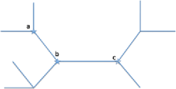
Figure 1: A 7-leaf Cladogram.

Consider the branchpoint $b$ in the $7$-leaf Cladogram $\mathbf{t}$ in Figure 1. It divides the collection of leaves naturally into three sets. Let $X(\mathbf{t})=(X_{1},X_{2},\break X_{3})(\mathbf{t})$ denote the vector of proportion of leaves in each set. The corresponding number of edges in these sets are $(2nX_{1}-1,2nX_{2}-1,2nX_{3}-1)$. For example, at time zero in our given tree, going clockwise from the right we have $X(0)=(3/7,2/7,2/7)$.

Let $\mathbb{S}_{n}$ denote the unit simplex

$$\mathbb{S}_{n}=\Biggl{\{}x\in\mathbb{R}^{n}\dvtx x_{i}\geq 0\mbox{ for all $i$ and }\sum_{i=1}^{n}x_{i}=1\Biggr{\}}.$$ (1)

Some simple algebra will reveal that for any point $x=(x_{1},x_{2},x_{3})$ in $\mathbb{S}_{3}$, given $X(\mathbf{t})=x$, the difference $X_{1}(\mathbf{t}^{\prime})-X_{1}(\mathbf{t})$ can only take values in $\{-1/n,0,1/n\}$ with corresponding probabilities

$$q_{x_{1}}=x_{1}\frac{2n(1-x_{1})-2}{2n-5},\qquad 1-p_{x_{1}}-q_{x_{1}},\qquad p_{x_{1}}=(1-x_{1})\frac{2nx_{1}-1}{2n-5}.$$

Thus

$$\quad E\bigl{(}X_{1}(\mathbf{t}^{\prime})-X_{1}(\mathbf{t})\mid X(\mathbf{t})=x\bigr{)} = \frac{1}{n}\frac{2x_{1}-(1-x_{1})}{2n-5}\approx-\frac{1}{n^{2}}\frac{1}{2}(1-3x_{1}),$$

$$\quad E\bigl{(}\bigl{(}X_{1}(\mathbf{t}^{\prime})-X_{1}(\mathbf{t})\bigr{)}^{2}\mid X(\mathbf{t})=x\bigr{)} = \frac{1}{n^{2}}\frac{4nx_{1}(1-x_{1})-x_{1}-1}{2n-5}$$ (2)

$$\approx \frac{1}{n^{2}}2x_{1}(1-x_{1}).$$

If we take scaled limits, as $n$ goes to infinity, of the first two conditional moments (the mixed moments can be similarly verified), it is intuitive (and follows by standard tools) that as $n$ goes to infinity, this Markov chain (run at $n^{2}/2$ speed) will converge to a diffusion with a generator

$$\frac{1}{2}\sum_{i,j=1}^{3}x_{i}(1\{i=j\}-x_{j})\frac{\partial^{2}}{\partial x_{i}\,\partial x_{j}}-\frac{1}{2}\sum_{i=1}^{n}\frac{1}{2}(1-3x_{i})\frac{\partial}{\partial x_{i}}.$$ (3)

The generator written as above is similar to the generator for the well-known diffusion limit of the Wright–Fisher (WF) Markov chain models in population genetics. The WF model is one of the most popular models in population genetics. This is a multidimensional Markov chain which keeps track of the vector of proportions of certain genetic traits in a population of nonoverlapping generations. A good source for an introduction to these models is Chapter 1 in the book by Durrett durrettgenetics . For computational purposes one often takes recourse to a diffusion approximation, which, in its standard form, leads to a family of diffusions parametrized by $n$ “mutation rates.” The state space of the diffusion is given by $\mathbb{S}_{n}$ and is parametrized by a vector $(\delta_{1},\ldots,\delta_{n})$ of nonnegative entries. A weak solution of the WF diffusion with parameters $\delta=(\delta_{1},\ldots,\delta_{n})$ solves the following stochastic differential equation for $i=1,2,\ldots,n$:

$$dJ_{i}(t)=\frac{1}{2}\bigl{(}\delta_{i}-\delta_{0}J_{i}(t)\bigr{)}\,dt+\sum_{j=1}^{n}\tilde{\sigma}_{i,j}(J)\,d\beta_{j}(t),\qquad\delta_{0}=\sum_{i=1}^{n}\delta_{i}.$$ (4)

Here $\beta=(\beta_{1},\ldots,\beta_{n})$ is a standard multidimensional Brownian motion, and the diffusion matrix $\tilde{\sigma}$ is given by

$$\tilde{\sigma}_{i,j}(x)=\sqrt{x_{i}}\bigl{(}1\{i=j\}-\sqrt{x_{i}x_{j}}\bigr{)},\qquad 1\leq i,j\leq n.$$ (5)

We define the Wright–Fisher diffusion with negative mutation rates to be a family of $n$-dimensional diffusions, parametrized by $n$ nonnegative parameters $\delta=(\delta_{1},\ldots,\delta_{n})$, which is a weak solution of the following differential equation:

$$d\mu_{i}(t)=-\frac{1}{2}\bigl{(}\delta_{i}-\delta_{0}\mu_{i}(t)\bigr{)}\,dt+\sum_{j=1}^{n}\tilde{\sigma}_{i,j}(\mu)\,d\beta_{j}(t),\qquad\delta_{0}=\sum_{i=1}^{n}\delta_{i}.$$ (6)

The initial condition $\mu(0)$ is in the interior of $\mathbb{S}_{n}$ and the process has a drift that pushes it outside the simplex. We will show later that the process is sure to hit the boundary of the simplex at which point we stop it. In the next section we will explicitly construct a weak solution of (6). The uniqueness in law of such a solution, until it hits the boundary, follows since the drift and the diffusion coefficients are smooth (hence, Lipschitz) inside the open unit simplex. The law of this process will then be denoted uniquely by $\operatorname{NWF}(\delta_{1},\ldots,\delta_{n})$.

Equivalently this process can be identified by its Markov generator. Expanding $\tilde{\sigma}\tilde{\sigma}^{\prime}$ and using the fact that $\sum_{i=1}^{n}x_{i}=1$, we get

$$\mathcal{A}_{n}=\frac{1}{2}\sum_{i,j=1}^{n}x_{i}(1\{i=j\}-x_{j})\frac{\partial^{2}}{\partial x_{i}\,\partial x_{j}}-\sum_{i=1}^{n}\frac{1}{2}(\delta_{i}-\delta_{0}x_{i})\frac{\partial}{\partial x_{i}},$$ (7)

which identifies (3) as the generator for $\operatorname{NWF}(1/2,1/2,1/2)$.

In this text we focus on properties of NWF models as a family of diffusions on the unit simplex and explore some of their properties that are important in the context of the Markov chain model on Cladograms.

Part (1). We show that, just like Wright–Fisher diffusions (see vsm ), the NWF processes can be recovered from a far simpler class of models, the Bessel-square (BESQ) processes with negative dimensions. A comprehensive treatment of BESQ processes can be found in the book by Revuz and Yor RY . This family of one-dimensional diffusions is indexed by a single real parameter $\theta$ (called the dimension) and are solutions of the stochastic differential equations

$$Z(t)=x+2\int_{0}^{t}\sqrt{|Z(s)|}\,d\beta(s)+\theta t,\qquad x\geq 0,t\geq 0,$$ (8)

where $\beta$ is a one-dimensional standard Brownian motion. We denote the law of this process by $Q^{\theta}_{x}$. It can be shown that the above SDE admits a unique strong solution until it hits the origin. The classical model only admits paramater $\theta$ to be nonnegative. However, an extension, introduced by Göing-Jaeschke and Yor yornbesq , allows the parameter $\theta$ to be negative. It is important to note that $Q_{x}^{\theta}$ is the diffusion limit of a Galton–Watson branching process with a $|\theta|$ rate of immigration (for $\theta\geq 0$) or emigration (for $\theta<0$).

In Section 3 we show that the $\operatorname{NWF}(\delta_{1},\ldots,\delta_{n})$ law, starting at $(x_{1},\ldots,x_{n})$, can be recovered via a stochastic time-change from a collection of $n$ independent processes with laws $Q_{x_{i}}^{-2\delta_{i}}$, $i=1,\ldots,n$, and dividing each coordinate by the total sum. For the corresponding discrete models this is usually referred to as Poissonization.

In this article we utilize this relationship to infer several properties about the NWF processes. For example, we prove that these diffusions, almost surely, hit the boundary of the simplex. We derive the explicit exit density supported on the union of the boundary walls in Theorem 9.

Part (2). We also prove an interesting duality relationship between WF and NWF models. To describe the duality relationship we let the NWF continue in the lower dimensional simplex when any of the coordinates hit zero. Thus, every time a coordinate hits zero, the dimension of the process gets reduced by one, and ultimately the process is absorbed at the scalar one. Such a process can be obtained by running a WF model with appropriate parameters that initially starts with dimension one and value $1$. At independent random times, the dimension of the process increases by one, and the newly added coordinate is initialized at zero. Finally we condition on the values of the process at a chosen random time. The resulting process, backwards in time and suitably time-changed, is the original NWF model.

Part (3). The time that the NWF process takes to exit the simplex is a crucial quantity due to a reason which we describe below. We keep our exposition mostly verbal without going into too much detail since the details require considerable formalism from the theory of continuum trees and will be discussed elsewhere. In palCT we show how Part (1) points toward a Poissonization of the entire Aldous Markov chain, which is simpler for considering scaled limits. The Poissonized version of the Markov chain on $n$-leaf Cladograms stipulates: every existing leaf has an exponential clock of rate $2$ attached to it which determines the instances of their deaths, and every existing edge has an independent exponential clock of rate $1$ attached to it, at which point the edge is split, and a new pair of vertices (one of which is a leaf) is introduced. It is an easy verification that the rates are consistent with the BESQ limit that we claimed in Part (1) above. Hence, one would expect that the limit of the Poissonized chains on continuum trees, normalized to give a leaf-mass measure one, and suitably time-changed would give the conjectured Aldous diffusion. This is the strategy followed in palCT .

Now, the Poissonized chain has some beautiful and interesting structures. Please see A93 for the details about continuum trees that we use below. A continuum tree $\mathbb{T}$ comes with its associated (infinite) length measure (analogous to the Lebesgue measure) and a leaf-mass probability measure, which describes how the leaves are distributed on it. We will denote the length measure by $\mathbf{Leb}(\mathbb{T})$ and the leaf-mass probability measure by $\mu(\mathbb{T})$. Suppose we sample $n$ i.i.d. elements from $\mu(\mathbb{T})$ and draw the tree generated by them, which produces an $n$-leaf Cladogram with edge-lengths (or, a proper $n$-tree, according to A93 ). Thus, by using the fact that the continuum tree is compact, one can approximate a continuum tree by a sequence of $n$-leaf Cladograms.

Now consider an $n$-leaf Cladogram for a very large $n$, and further consider $m$ internal branchpoints. For example, in Figure 1, we have three branchpoints $\{a,b,c\}$ in a $7$-leaf Cladogram. These branchpoints generate a skeleton subtree of the original tree and partition the leaves as internal or external to the skeleton. The components of the vector of external leaf masses grow as independent continuous time, binary branching, Galton–Watson branching processes with a rate of branching/dying $2$ and a rate of emigration $1$. Note that this is consistent with the diffusion limit as BESQ with $\theta=-1$. As the Markov chain (Poissonized or not) proceeds, there comes a time when one of these external leaf masses gets exhausted. When this happens, one of the internal branch points becomes a leaf. The distribution of every coordinate of external leaf-masses at this exit time is derived in Part (2). Until this time, supported on the skeleton, new subtrees can grow and decay. We show, in palCT , that the dynamics of the sizes of these subtrees on the internal part can be modeled as the age process of a chronological splitting tree. Chronological splitting trees are a special kind of biological tree, where an individual lives up to a certain (possibly nonexponential) lifetime and produces children at rate one during that lifetime. Her children behave in an identical manner with an independent and identically distributed lifetime of their own. The age process refers to the point process of current ages of the existing members in the family. More details about splitting trees can be found in the article by Lambert lambertAOP .

When one of the internal vertices gets exposed, the above dynamics breaks down, and we need to find a slightly different set of internal vertices to proceed. Hence, it is important to derive estimates of the times at which this change happens. We provide quantitative bounds on the value of this stopping time under the special situation of symmetric choice of parameters, which is the case at hand.

The article is divided as follows. Our main tool in this analysis is to establish a relationship between NWF processes and Bessel-square processes of negative dimensions, much in the spirit of Pal vsm . This has been done in Section 3 where we also establish Theorem 7. The relevant results about BESQ processes have been listed in Section 2. Most of these results are known, and appropriate citations have been provided. Proofs of the rest can be found in the Appendix. Exact computations of exit density from the simplex have been done in Section 4. Estimates of the exit time have been established in Section 5.

2 Some results about BESQ processes

The Bessel-square processes of negative dimensions $-\theta$, where $\theta\geq 0$, are one-dimensional diffusions which are the unique strong solution of the SDE

$$X(t)=x-\theta t+2\int_{0}^{t}\sqrt{X(s)}\,d\beta(s),\qquad t\leq T_{0},$$ (9)

where $T_{0}$ is the first hitting time of zero for the process $X$, and $x$ is a positive constant. The process is absorbed at zero. We will denote the law of this process $Q_{x}^{-\theta}$ just as BESQ of a positive dimension $\theta$ will be denoted by $Q^{\theta}_{x}$.

The following collection of results is important for us. All the proofs can be found in the article by Göing-Jaeschke and Yor yornbesq .

Lemma 1 ((Time-reversal))

For any $\theta>-2$ and any $x>0$, $Q_{x}^{-\theta}(T_{0}<\infty)=1$, while for $\theta\geq 2$, one has $Q^{\theta}_{x}(T_{0}<\infty)=0$.

Moreover the following equality holds in distribution:

$$\bigl{(}X(T_{0}-u),u\leq T_{0}\bigr{)}=\bigl{(}Y(u),u\leq L_{x}\bigr{)},$$ (10)

where $Y$ has law $Q^{4+\theta}_{0}$, and $L_{x}$ is the last hitting time of $x$ for the process $Y$.

In particular: [(ii)]

Both $L_{x}$ and $T_{0}$ are distributed as $x/2G$, where $G$ is a Gamma random variable with parameter $(\theta/2+1)$.

The transition probabilities $p_{t}^{\theta}(x,y)$ for $x,y>0$ satisfy the identity

$$p_{t}^{-\theta}(x,y)=p_{t}^{4+\theta}(y,x).$$

The following results have been proved in the Appendix.

Lemma 2

The scale function for $Q^{-\theta}$, $\theta\geq 0$, is given by the function

$$s(x)=x^{\theta/2+1},\qquad x\geq 0.$$

Moreover: [(ii)]

The origin is an exit boundary for the diffusion and not an entry.

The change of measure

$$x^{-\theta/2-1}Q_{x}^{-\theta}(X(t)^{\theta/2+1}1(\cdot))$$

on the $\sigma$-algebra generated by the process up to time $t$ is consistent for various $t$ and is the law of $Q_{x}^{4+\theta}$. Thus, we say $Q_{x}^{4+\theta}$ is $Q_{x}^{-\theta}$ conditioned never to hit zero.

The previous fact is the generalization of the well-known observation that Brownian motion, conditioned never to hit the origin, has the law of the three-dimensional Bessel process.

Lemma 3

Let $\{Z(t),t\geq 0\}$ denote a BESQ process of dimension $\theta$ for some $\theta>2$. Then

$$\lim_{\varepsilon\rightarrow 0}\frac{1}{\log(1/\varepsilon)}\int_{\varepsilon}^{t}\frac{du}{Z(u)}=\frac{1}{\theta-2}\qquad\mbox{for all }t>0.$$

3 Changing and reversing time

Our objective in this section is to establish a time-reversal relationship between NWF and WF models.

Theorem 4

Let $z_{1},\ldots,z_{n}$ and $\theta_{1},\ldots,\theta_{n}$ be nonnegative constants. Let $Z=(Z_{1},\ldots,Z_{n})$ be a vector of $n$ independent BESQ processes of dimensions $-\theta_{1},\ldots,-\theta_{n}$, respectively, starting from $(z_{1},\ldots,z_{n})$. Let $\zeta$ be the sum $\sum_{i=1}^{n}Z_{i}$.

Define

$$T_{i}=\inf\{t\geq 0\dvtx Z_{i}(t)=0\},\qquad\tau=\bigwedge_{i=1}^{n}T_{i}.$$

Then, there is an $n$-dimensional diffusion $\mu$, satisfying the SDE in (6) for $\operatorname{NWF}(\theta_{1}/2,\ldots,\theta_{n}/2)$, for which the following equality holds:

$$Z_{i}(t\wedge\tau)=\zeta(t\wedge\tau)\mu_{i}(4C_{t}),\qquad 1\leq i\leq n,\qquad C_{t}=\int_{0}^{t\wedge\tau}\frac{ds}{\zeta(s)}.$$ (11)

Thus, in particular, equation (6) admits a weak solution for all nonnegative parameters $(\delta_{1},\ldots,\delta_{n})$.

The proof is almost identical to the case of WF model as shown in vsm , Proposition 11, with obvious modifications. For example, unlike the WF case, the time-change clock is no longer independent of the NWF process. We outline the basic steps below.

We know from (9) that

$$dZ_{i}(t\wedge\tau)=-\theta_{i}d(t\wedge\tau)+2\sqrt{Z_{i}}\,d\beta_{i}(t\wedge\tau),\qquad i=1,2,\ldots,n.$$

Define $\theta_{0}=\sum_{i=1}^{n}\theta_{i}$. Let $V_{i}(t)=Z_{i}/\zeta(t)$ for $t\leq\tau$. Then by Itô’s rule, we get

$$dV_{i}(t\wedge\tau)=-\zeta^{-1}[\theta_{i}-\theta_{0}V_{i}]\,d(t\wedge\tau)+\sqrt{{V_{i}}(1-V_{i})}\,dM_{i}(t),$$ (12)

where

$$dM_{i}(t)=\frac{2\zeta^{-1/2}}{\sqrt{1-V_{i}}}\sum_{j=1}^{n}\bigl{(}1\{i=j\}-\sqrt{V_{i}V_{j}}\bigr{)}\,d\beta_{j}(t\wedge\tau),$$ (13)

and $\langle M_{i}\rangle(t)=4C_{t}$.

Let $\{\rho_{u},u\geq 0\}$ be the inverse of the increasing function $4C_{t}$. Applying this time-change to the SDE for $V_{i}$ in (12), we get

$$d\mu_{i}(t)=-\tfrac{1}{4}[\theta_{i}-\theta_{0}\mu_{i}]\,dt+\sqrt{\mu_{i}(1-\mu_{i})}\widetilde{W}_{i}(t),$$ (14)

where $\widetilde{W}_{i}$ is the Dambis–Dubins–Schwarz (DDS; see RY , page 181) Brownian motion associated with $M_{i}$. This turns out to be the SDE for $\operatorname{NWF}(\theta_{1}/2,\break\ldots,\theta_{n}/2)$.

Let $\theta_{1},\theta_{2},\ldots,\theta_{n}$ be nonnegative and $z_{1},z_{2},\ldots,z_{n}$ be positive constants. For $i=1,2,\ldots,n$ define independent random variables $(G_{1},\ldots,G_{n})$ where $G_{i}$ is distributed as $\operatorname{Gamma}(\theta_{i}/2+1)$. Let

$$R_{i}=\frac{z_{i}}{2G_{i}},\qquad i=1,2,\ldots,n.$$ (15)

Also, independent of $(G_{1},\ldots,G_{n})$, let $Y_{1},Y_{2},\ldots,Y_{n}$ be $n$ independent BESQ processes of positive dimensions $(4+\theta_{1}),(4+\theta_{2}),\ldots,(4+\theta_{n})$, respectively, all of which are starting from zero.

For any permutation $\pi$ of $n$ labels, condition on the event

$$R_{\pi_{1}}>R_{\pi_{2}}>\cdots>R_{\pi_{n}}\quad\mbox{and let}\quad R^{*}=R_{\pi_{2}}.$$ (16)

We now construct the following $n$ dimensional process $(X_{1},\ldots,X_{n})$:

$$X_{i}(t)=Y_{i}\bigl{(}(t-R^{*}+R_{i})^{+}\bigr{)},\qquad t\geq 0.$$ (17)

Notice that at time $t=0$, every $X_{i}$ is at zero except the $\pi_{1}$th.

Let $S(t)$ denote the total sum process $\sum_{i=1}^{n}X_{i}(t)$. Note that $S(t)>0$ for all $t\geq 0$ with probability one. Define the process

$$C_{t}:=\int_{0}^{t}\frac{du}{S(u)},\qquad t>0.$$ (18)

The process $C_{t}$ is finite almost surely for every $t$ (unfortunately, we cannot define $R^{*}=R_{\pi_{1}}$ precisely because $C_{t}$ will be infinity; see Lemma 3). Let $A$ denote the inverse function of the continuous increasing function $4C$. That is,

$$A_{t}=\inf\{u\geq 0\dvtx 4C_{u}\geq t\},\qquad t\geq 0.$$ (19)

Lemma 5

There is an $n$-dimensional diffusion $\nu$ such that the following time-change relationship holds:

$$\nu_{i}(t)=\frac{X_{i}}{S}(A_{t})\quad\mbox{or}\quad X_{i}(t)=S(t)\nu_{i}(4C_{t}),\qquad t\geq 0.$$ (20)

The distribution of $\nu$ is supported on the unit simplex

$$\mathbb{S}_{n}=\{x_{i}\geq 0\dvtx x_{1}+x_{2}+\cdots+x_{n}=1\}.$$

Conditional on the values of $G_{1},\ldots,G_{n}$ and the process $S$, the law of $\nu$ can be described as below.

Let $\pi$ be any permutation of $n$ labels. On the event $R_{\pi_{1}}>R^{*}=R_{\pi_{2}}>\cdots>R_{\pi_{n}}$. Let $V_{2}<\cdots<V_{n}$ be defined by

$$A_{V_{i}}=R^{*}-R_{\pi_{i}}\quad\mbox{or, equivalently}\quad 4C_{R^{*}-R_{\pi_{i}}}=V_{i}.$$

Note that $V_{2}=0$.

For $i\geq 2$ and $V_{i}\leq t\leq V_{i+1}$, the process $\nu$ is zero on all coordinates except $(\pi_{1},\ldots,\pi_{i})$. The process $\nu(\pi_{1},\ldots,\pi_{i})$, given the history of the process till time $V_{i}$ (and the $G_{i}$’s and $S$), is distributed as the classical Wright–Fisher diffusion starting from

$$\frac{1}{S}(X_{\pi_{1}},\ldots,X_{\pi_{i}})(A_{V_{i}})=\frac{1}{S}(X_{\pi_{1}},\ldots,X_{\pi_{i}})(R^{*}-R_{\pi_{i}}),$$

and with parameters $(\gamma_{\pi_{1}},\ldots,\gamma_{\pi_{i}})$ where

$$\gamma_{j}=\theta_{j}/2+2,\qquad j=1,2,\ldots,n.$$

The Gamma random variables $G_{1},\ldots,G_{n}$ are independent of the BESQ process $Y_{1},\ldots,Y_{n}$. Thus, conditional on $G_{1},\ldots,G_{n}$, the vector of processes $(X_{1},\ldots,X_{n})$ has the following description. For

$$R^{*}-R_{\pi_{i}}\leq t\leq R^{*}-R_{\pi_{i+1}},\qquad i\geq 2,$$

all coordinates other than the $\pi_{1}$th, $\pi_{2}$th, …, $\pi_{i}$th are zero. And, $(X_{\pi_{1}},\ldots,\break X_{\pi_{i}})$, conditioned on the past, are independent BESQ processes of dimensions $(4+\theta_{\pi_{1}},\ldots,4+\theta_{\pi_{i}})$ and starting from $(X_{\pi_{1}},\ldots,X_{\pi_{i}})(R^{*}-R_{\pi_{i}})$.

Thus, on this interval of time, the existence of the process $\nu$, identifying its law as the WF law, and the claimed independence from the process $S$, all follow from vsm , Proposition 11. The proof of the lemma now follows by combining the argument over the distinct intervals.

Lemma 6

Consider the set-up in (15), (17) and (19). Let $Z_{1},Z_{2},\ldots,Z_{n}$ be $n$ stochastic processes defined such that $\{Z_{i}(t),0\leq t\leq R^{*}\}$ is the time-reversal of the process $\{X_{i}(t),0\leq t\leq R^{*}\}$, conditioned on $X_{i}(R^{*})=z_{i}$. That is, conditioned on $X_{i}(R^{*})=z_{i}$ for every $i$,

$$Z_{i}(t)=X_{i}(R^{*}-t)=Y_{i}(R_{i}-t)^{+}\qquad\mbox{for }0\leq t\leq R^{*}.$$

Then $(Z_{1},\ldots,Z_{n})$ are independent BESQ processes of dimensions $-\theta_{1},\ldots,\break-\theta_{n}$, starting from $z_{1},\ldots,z_{n}$, and absorbed at the origin.

It suffices to prove the following:

Let $\{Y(t),t\geq 0\}$ denote a BESQ process of dimension $(4+\theta)$ starting from $0$. Fix a $z>0$. Let $T$ be distributed as $z/2G$, where $G$ is a Gamma random variable with parameter $(\theta/2+1)$. Then, conditioned on $T=l$ and $Y(l)=z$, the time-reversed process $\{Y((l-s)^{+}),0\leq s<\infty\}$ is distributed as $Q_{z}^{-\theta}$, absorbed at the origin, conditioned on $T_{0}=l$. Here $T_{0}$ is the hitting time of the origin for $Q_{z}^{-\theta}$.

Once we prove this claim, the lemma follows since the law of $T_{0}$ is exactly $z/2G$. See Lemma 1.

Proof of Claim For the case of $\theta=0$, this is proved in besselbridge , page 447. The general proof is exactly similar and we outline just the steps and give references within besselbridge for the details.

For any $\theta\in\mathbb{R}$, $t>0$, $x,y\geq 0$, let $Q^{\theta,t}_{x\rightarrow y}$ denote the law of the BESQ bridge of dimension $\theta$, length $t$, from points $x$ to $y$. That is to say, if $Y$ follows $Q_{x}^{\theta}$, then $Q^{\theta,t}_{x\rightarrow y}$ is the law of the process $\{Y(s),0\leq s\leq t\}$ conditioned on the event $\{Y(t)=y\}$.

Now, BESQ bridges satisfy time-reversal besselbridge , page 446. Thus, if we define $\widehat{P}$ to be the $P$-distribution of a process $\{X(t-s),0\leq s\leq t\}$, then $Q^{\theta,t}_{x\rightarrow y}=\widehat{Q}^{\theta,t}_{y\rightarrow x}$.

We consider the case when the dimension is $(4+\theta),\theta\geq 0$, $x=0,y=z>0$. Then

$$Q^{4+\theta,t}_{z\rightarrow 0}=\widehat{Q}^{4+\theta,t}_{0\rightarrow z}.$$

Now, from Lemma 2 (also see besselbridge , Section 3, page 440), we know that $Q^{4+\theta}_{z}$ is $Q^{-\theta}_{z}$ conditioned never to hit zero (or equivalently, $Q^{-\theta}_{z}$ can be interpreted as $Q_{z}^{4+\theta}$ conditioned to hit zero). Since the origin is an exit distribution for $Q^{-\theta}_{z}$ and not an entry (Lemma 2; see besselbridge , page 441, for the details of these definitions), the conditional law $Q^{4+\theta,t}_{z\rightarrow 0}$ is nothing but $Q^{-\theta}_{z}$, conditioned on $T_{0}=t$. This completes the proof.

The following is a more precise statement.

Let $(z_{1},\ldots,z_{n})$ be a point in the $n$-dimensional unit simplex $\mathbb{S}_{n}$. Fix $n$ nonnegative parameters $\delta_{1},\ldots,\delta_{n}$. Let $G_{1},\ldots,G_{n}$ denote $n$ independent Gamma random variables with parameters $\delta_{1}+1,\ldots,\delta_{n}+1$, respectively. Define $R_{i}=z_{i}/2G_{i}$.

For any permutation $\pi$ of $n$ labels, condition on the event $R_{\pi_{1}}>R_{\pi_{2}}>\cdots>R_{\pi_{n}}$, and let $R^{*}=R_{\pi_{2}}$.

Define the continuous process $S$ by prescribing $S(0)=Z_{1}(R_{\pi_{1}}-R^{*})$ where $Z_{1}$ is distributed as $Q_{0}^{4+2\delta_{\pi_{1}}}$, and for any $t$ such that

$$R^{*}-R_{\pi_{i}}\leq t\leq R^{*}-R_{\pi_{i+1}},\qquad i\geq 2,\qquad R_{\pi_{n+1}}=0.$$

Given the history, the process is distributed as a Bessel-square process of dimension $\sum_{j=1}^{i}(4+2\delta_{\pi_{j}})$ starting from $S(R^{*}-R_{\pi_{i}})$.

Define the stochastic clocks

$$C_{t}=\int_{0}^{t}\frac{du}{S(u)},\qquad\widehat{C}_{t}=\int_{R^{*}-t}^{R^{*}}\frac{du}{S(u)},\qquad 0\leq t\leq R^{*},$$

and let $\widehat{A}_{t}$ denote the inverse function of $4\widehat{C}_{t}$. Let $V_{2}<\cdots<V_{n}$ be defined by $4C_{R^{*}-R_{\pi_{i}}}=V_{i}$. Note that $V_{2}=0$. The $4$ is a standardization constant that appears due to the factor of $2$ in the diffusion coefficient in (8).

Define an $n$-dimensional process $\nu$, given $R_{1},\ldots,R_{n}$, and the process $S$. For $i\geq 2$ and $V_{i}\leq t\leq V_{i+1}$, the process $\nu$ is zero on all coordinates, except possibly at indices $(\pi_{1},\ldots,\pi_{i})$. At time zero, the process starts at the vector that is $1$ in the $\pi_{1}$th coordinate and zero elsewhere.

Conditioned on the history till time $V_{i}$, the process $\{\nu(\pi_{1},\ldots,\pi_{i})(t),V_{i}\leq t\leq V_{i+1}\}$ is distributed as the classical Wright–Fisher diffusion, starting from $\nu(\pi_{1},\ldots,\pi_{i})(V_{i})$ and with parameters $(\gamma_{\pi_{1}},\ldots,\gamma_{\pi_{i}})$, where

$$\gamma_{j}=\delta_{j}+2,\qquad j=1,2,\ldots,n.$$

Finally, consider the conditional law of the process, conditioned on the event

$$S(R^{*})\nu_{i}(4C_{R^{*}})=z_{i}\qquad\mbox{for all }i=1,2,\ldots,n.$$

Theorem 7

Define the time-reversed process

$$\mu(t)=\nu(\widehat{A}\circ 4C_{R^{*}-t}),$$

where $\circ$ denotes composition. Then this conditional stochastic time-reversed process, until the first time any of the coordinates hit zero, has a marginal distribution (when $G_{i}$’s and $S$ are integrated out) $\operatorname{NWF}(\delta_{1},\ldots,\delta_{n})$ starting from $(z_{1},\ldots,z_{n})$.

We start with given values of $R_{\pi_{1}}>R_{\pi_{2}}>\cdots>R_{\pi_{n}}$ and the process $S$ and apply equation (20) in Lemma 5 to obtain the processes $(X_{1},\ldots,X_{n})$, defined by

$$X_{i}(t)=S(t)\nu_{i}(4C_{t}),\qquad 0\leq t\leq R^{*}.$$

Then, the vector $(X_{1},X_{2},\ldots,X_{n})$ has the law prescribed by (17).

Now we apply Lemma 6 to obtain $(Z_{1},\ldots,Z_{n})$ by conditioning $(X_{1},\ldots,X_{n})$ and reversing time. Finally the construction in Theorem 4 gives us the vector $(\mu_{1},\ldots,\mu_{n})$ from $(Z_{1},\ldots,Z_{n})$, as desired.

4 Exit density

Let $Z_{1},Z_{2},\ldots,Z_{n}$ be independent BESQ processes of dimensions $-\theta_{1},\ldots,-\theta_{n}$, where each $\theta_{i}\geq 0$. We assume that at time zero, the vector $\mathbf{Z}=(Z_{1},\ldots,Z_{n})$ starts from a point $\mathbf{z}=(z_{1},\ldots,z_{n})$ where every $z_{i}>0$. Define $T_{i}$ to be the first hitting time of zero for the process $Z_{i}$, and let $\tau=\bigwedge_{i}T_{i}$ denote the first time any coordinate hits zero. We would like to determine the joint distribution of $(\tau,\mathbf{Z}(\tau))$.

Note that since each $T_{i}$ is a continuous random variable, the minimum is attained at a unique $i$. Thus, for a fixed $1\leq i\leq n$, conditioned on the event $\tau=T_{i}$, the distribution of $Z_{i}(\tau)$ is the unit mass at zero, and the distribution of every other $Z_{j}(\tau)$ is supported on $(0,\infty)$. Now, let $h_{i}$ denote the density of the stopping time $T_{i}$ on $(0,\infty)$, and let $q_{t}^{-\theta}$ refer to the transition density of $Q^{-\theta}$. It follows that for any $a_{j}>0$, $j\neq i$, we get

$$P\bigl{(}\tau=T_{i},\tau\leq t,Z_{j}(\tau)\geq a_{j}\mbox{ for all $j\neq i$}\bigr{)}$$

$$\qquad=P\bigl{(}T_{i}\leq t,T_{j}>T_{i},Z_{j}(T_{i})\geq a_{j}\mbox{ for all $j\neq i$}\bigr{)}$$

$$\qquad=\int_{0}^{t}h_{i}(s)\prod_{j\neq i}P\bigl{(}T_{j}>s,Z_{j}(s)\geq a_{j}\bigr{)}\,ds=\int_{0}^{t}h_{i}(s)\prod_{j\neq i}P\bigl{(}Z_{j}(s)\geq a_{j}\bigr{)}\,ds$$

$$\eqntext{\mbox{since $a_{j}>0$}}$$

$$\qquad=\int_{0}^{t}h_{i}(s)\biggl{[}\prod_{j\neq i}\int_{a_{j}}^{\infty}q_{s}^{-\theta_{j}}(z_{j},y_{j})\,dy_{j}\biggr{]}\,ds.$$

Our first job is to find closed form expressions of the integral above. To do this we start by noting that $T_{i}$ is distributed as $z_{i}/2G_{i}$ (see Lemma 1), where $G_{i}$ is a Gamma random variable with parameter $(4+\theta_{i})/2-1=\theta_{i}/2+1$. That is, the density of $G_{i}$ is supported on $(0,\infty)$ and is given by

$$\frac{y^{\theta_{i}/2}}{\Gamma(\theta_{i}/2+1)}e^{-y}.$$

It follows that

$$h_{i}(s)=\frac{(z_{i}/2)^{\theta_{i}/2+1}}{\Gamma(\theta_{i}/2+1)}s^{-\theta_{i}/2-2}e^{-z_{i}/2s},\qquad 0\leq s<\infty.$$

On the other hand, it follows from time reversal (Lemma 1) that $q_{s}^{-\theta_{j}}(z_{j},\break y_{j})=q_{s}^{4+\theta_{j}}(y_{j},z_{j})$. For any positive $a$, the transition density $q^{a}_{s}(y,z)$ is explicitly known (see, e.g., vsm ) to be $s^{-1}f(z/s,a,y/s)$, where $f(\cdot,k,\lambda)$ is the density of a noncentral Chi-square distribution with $k$-degrees of freedom and a noncentrality parameter value $\lambda$. In particular, it can be written as a Poisson mixture of central Chi-square (or, Gamma) densities. Thus we have the following expansion:

$$\qquad q_{s}^{-\theta_{j}}(z_{j},y_{j})=q_{s}^{4+\theta_{j}}(y_{j},z_{j})=s^{-1}\sum_{k=0}^{\infty}e^{-y_{j}/2s}\frac{(y_{j}/2s)^{k}}{k!}g_{\theta_{j}+4+2k}(z_{j}/s),$$ (22)

where $g_{r}$ is the Gamma density with parameters $(r/2,1/2)$. That is,

$$g_{r}(x)=\frac{2^{-r/2}x^{r/2-1}}{\Gamma(r/2)}e^{-x/2},\qquad x\geq 0.$$

Now, define

$$\vec{y}_{i}=\sum_{j\neq i}y_{j},\qquad\vec{\theta}_{i}=\sum_{j\neq i}\theta_{j},\qquad\vec{z}_{i}=\sum_{j\neq i}z_{j}.$$

Thus

$$h_{i}(s)\prod_{j\neq i}q_{s}^{-\theta_{j}}(z_{j},y_{j})$$

$$\qquad=\frac{(z_{i}/2)^{\theta_{i}/2+1}}{\Gamma(\theta_{i}/2+1)}s^{-\theta_{i}/2-2}e^{-z_{i}/2s}\prod_{j\neq i}s^{-1}\sum_{k=0}^{\infty}e^{-y_{j}/2s}\frac{(y_{j}/2s)^{k}}{k!}g_{\theta_{j}+4+2k}(z_{j}/s)$$

$$\qquad=\frac{(z_{i}/2)^{\theta_{i}/2+1}}{\Gamma(\theta_{i}/2+1)}s^{-\theta_{i}/2-2}e^{-z_{i}/2s}$$

$$\qquad\quad{}\times\prod_{j\neq i}s^{-1}\sum_{k=0}^{\infty}e^{-y_{j}/2s}\frac{(y_{j}/2s)^{k}}{k!}\frac{2^{-\theta_{j}/2-2-k}(z_{j}/s)^{\theta_{j}/2+k+1}}{\Gamma(\theta_{j}/2+2+k)}e^{-z_{j}/2s}$$

$$\qquad=\frac{(z_{i}/2)^{\theta_{i}/2+1}}{\Gamma(\theta_{i}/2+1)}s^{-\theta_{i}/2-2-(n-1)}e^{-z_{i}/2s}$$

$$\qquad\quad{}\times e^{-(\vec{y}_{i}+\vec{z}_{i})/2s}2^{-\vec{\theta}_{i}/2-2(n-1)}\prod_{j\neq i}\sum_{k=0}^{\infty}\frac{(y_{j}/2s)^{k}}{k!}\frac{2^{-k}(z_{j}/s)^{\theta_{j}/2+k+1}}{\Gamma(\theta_{j}/2+2+k)}.$$

We now exchange the product and the sum in the above. We will need some more notations for a compact representation. For any two vectors $a$ and $b$, denote by

$$a^{b}=\prod_{i}a_{i}^{b_{i}},\qquad a!=\prod_{i}a_{i}!.$$

Also let $\bm{\Theta}_{i},\mathbf{y}_{i},\mathbf{z}_{i}$ stand for the vectors $(\theta_{j},j\neq i)$, $(y_{j},j\neq i)$ and $(z_{j},j\neq i)$, respectively.

Let $\mathbf{k}$ denote the vector $(k_{j},j\neq i)$, where every $k_{j}$ takes any nonnegative integer values. Let $\mathbf{k}^{\prime}1$ be the sum of the coordinates of $\mathbf{k}$. Then

$$\prod_{j\neq i}\sum_{k=0}^{\infty}\frac{(y_{j}/2s)^{k}}{k!}\frac{2^{-k}(z_{j}/s)^{\theta_{j}/2+k+1}}{\Gamma(\theta_{j}/2+2+k)}$$

$$\qquad=\sum_{N=0}^{\infty}(4s)^{-N}s^{-\vec{\theta}_{i}/2-N-(n-1)}\mathbf{z}_{i}^{\bm{\Theta}_{i}/2+1}\sum_{\mathbf{k}^{\prime}1=N}\frac{\mathbf{y}_{i}^{\mathbf{k}}}{\mathbf{k}!}\frac{\mathbf{z}_{i}^{\mathbf{k}}}{\prod_{j\neq i}\Gamma(\theta_{j}/2+2+k_{j})}.$$

Thus, combining the expressions, we get

$$h_{i}(s)\prod_{j\neq i}q_{s}^{-\theta_{j}}(z_{j},y_{j})$$

$$\qquad=\frac{z_{i}^{\theta_{i}/2+1}}{\Gamma(\theta_{i}/2+1)}2^{-\theta_{i}/2-1-\vec{\theta}_{i}/2-2(n-1)}$$ (23)

$$\qquad\quad{}\times s^{-\theta_{i}/2-2-(n-1)}e^{-z_{i}/2s}e^{-(\vec{y}_{i}+\vec{z}_{i})/2s}\sum_{N=0}^{\infty}4^{-N}s^{-\vec{\theta}_{i}/2-2N-(n-1)}B_{N},$$

where

$$B_{N}=\mathbf{z}_{i}^{\bm{\Theta}_{i}/2+1}\sum_{\mathbf{k}^{\prime}1=N}\frac{\mathbf{y}_{i}^{\mathbf{k}}}{\mathbf{k}!}\frac{\mathbf{z}_{i}^{\mathbf{k}}}{\prod_{j\neq i}\Gamma(\theta_{j}/2+2+k_{j})}.$$

We can now integrate over $s$ in (4) to obtain

$$\int_{0}^{\infty}h_{i}(s)\prod_{j\neq i}q_{s}^{-\theta_{j}}(z_{j},y_{j})\,ds=\sum_{N=0}^{\infty}B^{\prime}_{N}\int_{0}^{\infty}s^{-a_{N}}e^{-b/s}\,ds,$$

where

$$B_{N}^{\prime} = \frac{z_{i}^{\theta_{i}/2+1}}{\Gamma(\theta_{i}/2+1)}2^{-\theta_{0}/2-2n+1}4^{-N}B_{N},\qquad\theta_{0}=\sum_{i=1}^{n}\theta_{i},$$ (24)

$$a_{N} = \theta_{i}/2+\vec{\theta}_{i}/2+2n+2N=\theta_{0}/2+2n+2N,$$ (25)

$$b = z_{i}/2+(\vec{y}_{i}+\vec{z}_{i})/2=(\vec{y}_{i}+z_{0})/2,\qquad z_{0}=\sum_{i=1}^{n}z_{i}.$$ (26)

Now a simple change of variable $w=1/s$ shows

$$\displaystyle\int_{0}^{\infty}s^{-a_{N}}e^{-b/s}\,ds=\int_{0}^{\infty}w^{a_{N}}e^{-bw}w^{-2}\,dw=\int_{0}^{\infty}w^{a_{N}-2}e^{-bw}\,dw,$$

$$\displaystyle\frac{\Gamma(a_{N}-1)}{b^{a_{N}-1}}\int_{0}^{\infty}\frac{b^{a_{N}-1}}{\Gamma(a_{N}-1)}w^{a_{N}-2}e^{-bw}\,dw=\frac{\Gamma(a_{N}-1)}{b^{a_{N}-1}}.$$

Since the $i$th coordinate of the exit point is zero, one can define $y_{i}=0$ and $y_{0}=\sum_{j=1}^{n}y_{j}=\vec{y}_{i}$ to simplify notation. Thus we obtain

$$\int_{0}^{\infty}h_{i}(s)\prod_{j\neq i}q_{s}^{-\theta_{j}}(z_{j},y_{j})\,ds$$

$$\qquad=\sum_{N=0}^{\infty}\frac{z_{i}^{\theta_{i}/2+1}}{\Gamma(\theta_{i}/2+1)}2^{-\theta_{0}/2-2n+1}4^{-N}B_{N}\frac{\Gamma(a_{N}-1)}{b^{a_{N}-1}}$$

$$\qquad=\frac{z_{i}^{\theta_{i}/2+1}\mathbf{z}_{i}^{\bm{\Theta}_{i}/2+1}}{\Gamma(\theta_{i}/2+1)}2^{-\theta_{0}/2-2n+1}\sum_{N=0}^{\infty}\bigl{(}(\vec{y}_{i}+z_{0})/2\bigr{)}^{-\theta_{0}/2-2n-2N+1}$$

$$\qquad\quad{}\times\Gamma(\theta_{0}/2+2n+2N-1)4^{-N}\sum_{\mathbf{k}^{\prime}1=N}\frac{\mathbf{y}_{i}^{\mathbf{k}}}{\mathbf{k}!}\frac{\mathbf{z}_{i}^{\mathbf{k}}}{\prod_{j\neq i}\Gamma(\theta_{j}/2+2+k_{j})}$$

$$\qquad=\frac{\mathbf{z}^{\bm{\Theta}/2+1}}{\Gamma(\theta_{i}/2+1)}2^{-\theta_{0}/2-2n+1}\sum_{N=0}^{\infty}(y_{0}+z_{0})^{-\theta_{0}/2-2n-2N+1}2^{\theta_{0}/2+2n+2N-1}$$

$$\qquad\quad{}\times\Gamma(\theta_{0}/2+2n+2N-1)4^{-N}\sum_{\mathbf{k}^{\prime}1=N}\frac{\mathbf{y}_{i}^{\mathbf{k}}}{\mathbf{k}!}\frac{\mathbf{z}_{i}^{\mathbf{k}}}{\prod_{j\neq i}\Gamma(\theta_{j}/2+2+k_{j})}$$

$$\qquad=\frac{\mathbf{z}^{\bm{\Theta}/2+1}}{\Gamma(\theta_{i}/2+1)}\sum_{N=0}^{\infty}(y_{0}+z_{0})^{-\theta_{0}/2-2n-2N+1}$$

$$\qquad\quad{}\times\Gamma(\theta_{0}/2+2n+2N-1)\sum_{\mathbf{k}^{\prime}1=N}\frac{\mathbf{y}_{i}^{\mathbf{k}}}{\mathbf{k}!}\frac{\mathbf{z}_{i}^{\mathbf{k}}}{\prod_{j\neq i}\Gamma(\theta_{j}/2+2+k_{j})}.$$

We have the following result.

Theorem 8

Let $Z_{1},Z_{2},\ldots,Z_{n}$ be independent BESQ processes of dimensions $-\theta_{1},\ldots,-\theta_{n}$, where each $\theta_{i}\geq 0$. Assume that $Z_{i}(0)=z_{i}(0)>0$, for every $i$.

The distribution of $(\tau,Z({\tau}))$ is supported on the set $(0,\infty)\times\bigcup_{i=1}^{n}H_{i}$, where $H_{i}$ is the subspace orthogonal to the $i$th canonical basis vector $e_{i}$. That is,

$$H_{i}=\{(y_{1},y_{2},\ldots,y_{n})\dvtx y_{i}=0\}.$$

[(ii)]

Let $G_{i},i=1,2,\ldots,n$ be independent Gamma random variables with parameters $\theta_{i}/2+1,i=1,2,\ldots,n$. The law of $\tau$ is the same as that of $\min_{i}\frac{z_{i}}{2G_{i}}$ and

$$P(\tau=T_{i})=P\biggl{(}\frac{G_{i}}{z_{i}}>\frac{G_{j}}{z_{j}}\mbox{ for all $j\neq i$}\biggr{)},$$

where $T_{i}$ is the first hitting time of $H_{i}$.

The restriction of the law of the random vector $Z(\tau)$, restricted to the hyperplane $H_{i}$, admits a density with respect to all the variables $y_{j}$’s, $j\neq i$, which is given by

$$= \frac{S^{1-\theta_{0}/2-2n}}{\Gamma(\theta_{i}/2+1)}\prod_{j=1}^{n}z_{j}^{\theta_{j}/2+1}\sum_{N=0}^{\infty}\Gamma(\theta_{0}/2+2n+2N-1)S^{-2N}$$

$${}\times\sum_{\sum_{j\neq i}k_{j}=N}\prod_{j\neq i}\frac{(y_{j}z_{j})^{k_{j}}}{k_{j}!\Gamma(\theta_{j}/2+2+k_{j})}.$$

Here

$$S=\sum_{i=1}^{n}(y_{i}+z_{i}),\qquad y_{i}=0,\qquad\theta_{0}=\sum_{i=1}^{n}\theta_{i}.$$

Using Theorem 4, we get that the exit distribution of $\operatorname{NWF}(\delta_{1},\ldots,\delta_{n})$, starting from a point $(z_{1},\ldots,z_{n})\in\mathbb{S}_{n}$, is the image under the map

$$x_{i}\mapsto\frac{x_{i}}{\sum_{j=1}^{n}x_{j}},\qquad 1\leq i\leq n,$$

of the exit density of independent BESQ processes of dimensions $-\theta_{1},\ldots,-\theta_{n}$, where each $\theta_{i}=2\delta_{i}$.

Theorem 9

The exit density of $\mu\sim$ $\operatorname{NWF}(\delta_{1},\ldots,\delta_{n})$ starting from $(z_{1},\ldots,z_{n})\in\mathbb{S}_{n}$ is supported on the set $\bigcup_{i=1}^{n}F_{i}$, where $F_{i}$ is the face $\{x\in\mathbb{S}_{n}:x_{i}=0\}$, and admits the following description: [(ii)]

Let $G_{i},i=1,2,\ldots,n$, be independent Gamma random variables with parameters $\delta_{i}+1,i=1,2,\ldots,n$. Then

$$P(\mbox{$\mu$ exits through $F_{i}$})=P\biggl{(}\frac{G_{i}}{z_{i}}>\frac{G_{j}}{z_{j}}\mbox{ for all $j\neq i$}\biggr{)}.$$ (28)

Let $\delta$ represent the vector $(\delta_{1},\ldots,\delta_{n})$, and let $\delta_{0}=\sum_{i=1}^{n}\delta_{i}$. The exit distribution of the process $\mu$, restricted to $F_{i}$, admits a density with respect to all the variables $x_{j}$’s, $j\neq i$, which is given by

$$(\delta_{i}+1)\sum_{N=0}^{\infty}\frac{\Gamma(N+n+\delta_{0})}{\Gamma(N+2n+\delta_{0})}\sum_{\sum_{j\neq i}k_{j}=N}\operatorname{Dir}_{n}(z;\mathbf{k}+\delta+\mathbf{2})\operatorname{Dir}_{n-1}(x;\mathbf{k}+\mathbf{1}).$$ (29)

Here the inner sum above is over all nonnegative integers $(k_{j},j\neq i)$, such that $\sum_{j\neq i}k_{j}=N$. The vector $\mathbf{k}$ represents a vector whose $j$th coordinate is $k_{j}$ for all $j\neq i$, and $\mathbf{k}_{i}=0$. The vectors $\mathbf{k}+\delta+\mathbf{2}$ and $\mathbf{k}+\mathbf{1}$ represent vector additions of $\mathbf{k}$, $\delta$ and the vector of all twos, and $\mathbf{k}$ and the vector of all ones, respectively. The factor $\operatorname{Dir}_{n-1}$ is a density with respect to the $(n-1)$-dimensional vector $(x_{j},j\neq i)$ with corresponding parameters $(\mathbf{k}_{j}+1,j\neq i)$. It can also be interpreted as the conditional density of the $n$-dimensional $\operatorname{Dir}_{n}(x;\mathbf{k}+1)$, conditioned on $x_{i}=0$.

Note that the density in (29) is a mixture of Dirichlet densities, strikingly similar to those appearing as transition probabilities of the Wright–Fisher diffusions themselves. See Griffiths griffiths79b , Barbour, Ethier and Griffiths BEG and Pal vsm .

Proof of Theorem 9 This is a straightforward integration. We have assumed that $\sum_{i}z_{i}=1$. Thus, $S=1+\sum_{j}y_{j}$; define $y_{0}=\sum_{j}y_{j}$, and

$$x_{j}=y_{j}/y_{0},\qquad 1\leq j\leq n.$$

Hence (8) simplifies to

$$= \frac{(1+y_{0})^{1-\theta_{0}/2-2n}}{\Gamma(\theta_{i}/2+1)}\prod_{j=1}^{n}z_{j}^{\theta_{j}/2+1}\sum_{N=0}^{\infty}\Gamma(\theta_{0}/2+2n+2N-1)(1+y_{0})^{-2N}$$

$${}\times y_{0}^{N}\sum_{\sum_{j\neq i}k_{j}=N}\prod_{j\neq i}\frac{(x_{j}z_{j})^{k_{j}}}{k_{j}!\Gamma(\theta_{j}/2+2+k_{j})}.$$

Now, to get to formula (29) we need to make a multivariate change of variables. Without loss of generality, let $i=n$. Then, for any $y\in F_{i}$, we have $y_{n}=0$. Define the change of variables

$$(y_{1},\ldots,y_{n-2},y_{n-1})\mapsto(y_{0},x_{1},\ldots,x_{n-2}).$$

In other words, $y_{i}=y_{0}x_{i}$ for all $i=1,2,\ldots,n-2$ and $y_{n-1}=y_{0}(1-x_{1}-\cdots-x_{n-2})$. The determinant of the well-known Jacobian matrix is given by $y_{0}^{n-2}$.

Thus, the density of $(x_{1},\ldots,x_{n})$ restricted to $F_{i}$ is given by

$$\frac{1}{\Gamma(\theta_{i}/2+1)}\prod_{j=1}^{n}z_{j}^{\theta_{j}/2+1}\sum_{N=0}^{\infty}\Gamma(\theta_{0}/2+2n+2N-1)$$

$$\qquad{}\times\int_{0}^{\infty}y^{N+n-2}(1+y)^{1-\theta_{0}/2-2n-2N}\,dy$$ (31)

$$\qquad{}\times\sum_{\sum_{j\neq i}k_{j}=N}\prod_{j\neq i}\frac{(x_{j}z_{j})^{k_{j}}}{k_{j}!\Gamma(\theta_{j}/2+2+k_{j})}.$$

The following formula is easily verifiable for $\alpha\geq 0$, $\beta>\alpha+1$:

$$\int_{0}^{\infty}y^{\alpha}(1+y)^{-\beta}\,dy=\int_{0}^{1}x^{\beta-\alpha-2}(1-x)^{\alpha}\,dx=B(\alpha+1,\beta-\alpha-1),$$

where $B$ refers to the Beta function.

In other words, (4) reduces to

$$\frac{1}{\Gamma(\theta_{i}/2+1)}\prod_{j=1}^{n}z_{j}^{\theta_{j}/2+1}\sum_{N=0}^{\infty}\Gamma(\theta_{0}/2+2n+2N-1)$$

$$\qquad{}\times B(N+n-1,N+n+\theta_{0}/2)\sum_{\sum_{j\neq i}k_{j}=N}\prod_{j\neq i}\frac{(x_{j}z_{j})^{k_{j}}}{k_{j}!\Gamma(\theta_{j}/2+2+k_{j})}.$$

We now change $\theta_{i}/2$ to $\delta_{i}$ and rewrite the above expression in terms of Dirichlet densities. We use the notations in the statement of Theorem 9: the vector $\mathbf{k}$ represents a vector whose $j$th coordinate is $k_{j}$ for all $j\neq i$, and $\mathbf{k}_{i}=0$. The vectors $\mathbf{k}+\delta+\mathbf{2}$ and $\mathbf{k}+\mathbf{1}$ represent vector additions of $\mathbf{k}$, $\delta$ and the vector of all twos, and $\mathbf{k}$ and the vector of all ones, respectively. The factor $\operatorname{Dir}_{n-1}$ is a density with respect to the $(n-1)$-dimensional vector $(x_{j},j\neq i)$ with corresponding parameters $(\mathbf{k}_{j}+1,j\neq i)$. It can also be interpreted as the conditional density of the $n$-dimensional $\operatorname{Dir}_{n}(x;\mathbf{k}+1)$, conditioned on $x_{i}=0$.

Hence, for any $(k_{j},j\neq i)$, integers

$$\frac{z_{i}^{\delta_{i}+1}}{\Gamma(\delta_{i}+1)}\prod_{j\neq i}\frac{z_{j}^{k_{j}+\delta_{j}+1}}{\Gamma(\delta_{j}+2+k_{j})}\frac{x_{j}^{k_{j}}}{k_{j}!}$$

$$\qquad=\frac{(\delta_{i}+1)}{\Gamma(\delta_{0}+N+2n)\Gamma(N+n-1)}$$

$$\qquad\quad{}\times\operatorname{Dir}_{n}(z;\mathbf{k}+\delta+\mathbf{2})\operatorname{Dir}_{n-1}(x;\mathbf{k}+\mathbf{1}).$$

Thus (4) reduces to

$$(\delta_{i}+1)\sum_{N=0}^{\infty}\frac{\Gamma(\delta_{0}+2n+2N-1)B(N+n-1,N+n+\delta_{0})}{\Gamma(\delta_{0}+N+2n)\Gamma(N+n-1)}$$

(33)

$$\qquad{}\times\sum_{\mathbf{k}^{\prime}\mathbf{1}=N}\operatorname{Dir}_{n}(z;\mathbf{k}+\delta+\mathbf{2})\operatorname{Dir}_{n-1}(x;\mathbf{k}+\mathbf{1}).$$

However,

$$\frac{\Gamma(\delta_{0}+2n+2N-1)B(N+n-1,N+n+\delta_{0})}{\Gamma(\delta_{0}+N+2n)\Gamma(N+n-1)}$$

$$\qquad=\frac{\Gamma(\delta_{0}+2n+2N-1)}{\Gamma(\delta_{0}+N+2n)\Gamma(N+n-1)}\frac{\Gamma(N+n-1)\Gamma(N+n+\delta_{0})}{\Gamma(2N+2n+\delta_{0}-1)}$$

$$\qquad=\frac{\Gamma(N+n+\delta_{0})}{\Gamma(N+2n+\delta_{0})}.$$

This completes the proof of formula (29).

The probability in (28) is a direct consequence of Theorem 8 conclusion (i).

5 Exit time

Let $X=(X_{1},\ldots,X_{n})$ be distributed as $\operatorname{NWF}(-\theta_{1}/2,\ldots,\break-\theta_{n}/2)$ starting from a point $(x_{1},\ldots,x_{n})$ in the unit simplex. Let $\sigma_{0}$ denote the stopping time

$$\sigma_{0}=\inf\{t\geq 0\dvtx X_{i}=0\mbox{ for some $i$}\}.$$

Our objective is to find estimates on the law of $\sigma_{0}$.

We will simplify the situation by assuming that all $x_{i}=1/n$ and all $\theta_{i}=\theta$. To this end we use the time-change relationship in Theorem 4. Let $Z=(Z_{1},\ldots,Z_{n})$ be independent BESQ processes starting from $(z_{1},\ldots,z_{n})$ as in the set-up of Theorem 4, where each $z_{i}$ is now one. Then

$$\sigma_{0}=4\int_{0}^{\tau}\frac{ds}{\zeta(s)},\qquad\zeta(s)=\sum_{i=1}^{n}Z_{i}(s).$$ (34)

By Theorem 8, the distribution of $\tau$ is the same as considering $n$ i.i.d. $\operatorname{Gamma}(\theta/2+1)$ random variables $G_{1},\ldots,G_{n}$, and defining

$$\tau=\frac{1}{2\max_{i}G_{i}}.$$ (35)

Our first step will be to prove a concentration estimate of $\max_{i}G_{i}$.

Lemma 10

Let $G_{1},G_{2},\ldots,G_{n}$ be $n$ i.i.d. Gamma random variables with parameter $r/2$, for some $r\geq 2$. Let $\chi$ be the random variable $\max_{i}G_{i}$. Then, as $n$ tends to infinity,

$$E\sqrt{\chi}=\Theta\bigl{(}\sqrt{\log n}\bigr{)}.$$

First let $r\in\mathbb{N}$. Let $\{Z_{1}(i),\ldots,Z_{n}(i),i=1,2,\ldots,r\}$ be a collection of i.i.d. standard Normal random variables. Then $2G_{j}$ has the same law as $Z_{j}^{2}(1)+\cdots+Z_{j}^{2}(r)$. Hence

$$E\max_{j}|Z|_{j}(1)\leq E\sqrt{2\chi}\leq\sqrt{r}E\max_{i,j}|Z|_{j}(i).$$

As $n$ tends to infinity, the right-hand side above converges to $\sqrt{2r\log(rn)}$ while the left-hand side converges to $\sqrt{2\log n}$. This completes the argument for $r\in\mathbb{N}$. For a general positive $r$, bound on both sides by $\lfloor r\rfloor$ and $\lfloor r\rfloor+1$.

We also need a version of logarithmic Sobolev inequality for Gamma random variables, which can be found in several articles, including BW .

Lemma 11 ((BW , page 2718))

Let $\mu^{\theta}$ denote the product probability measure of $n$ i.i.d. $\operatorname{Gamma}(\theta)$ random variables. Then, for every $f$ on $\mathbb{R}^{n}$ which is in $C^{1}$ (i.e., once continuously differentiable), one has

$$\mathrm{Ent}(f^{2})\leq 4\int\Biggl{(}\sum_{i=1}^{n}x_{i}(\partial_{i}f(x))^{2}\Biggr{)}\,d\mu^{\theta}(x).$$ (36)

Here $\mathrm{Ent}(\cdot)$ refers to the entropy defined by

$$\mathrm{Ent}(f^{2})=\int f^{2}\log(f^{2})\,d\mu^{\theta}-\biggl{(}\int f^{2}\,d\mu^{\theta}\biggr{)}\log\biggl{(}\int f^{2}\,d\mu^{\theta}\biggr{)}.$$

And $\partial_{i}$ refers to the partial derivative with respect to the $i$th coordinate.

Lemma 12

Consider the set-up in Lemma 11. Let $F$ be a function on the open positive quadrant (i.e., every $x_{i}>0$) which is $C^{1}$ and satisfies

$$\sum_{i=1}^{n}x_{i}(\partial_{i}F)^{2}\leq F.$$ (37)

Then the following concentration estimate holds for any $r>0$:

$$\mu^{\theta}\bigl{(}\sqrt{F}-E_{\theta}\sqrt{F}\geq r\bigr{)} \leq\exp(-r^{2}),\qquad\mu^{\theta}\bigl{(}\sqrt{F}-E_{\theta}\sqrt{F}\leq-r\bigr{)}\leq\exp(-r^{2}),$$

where $E_{\theta}\sqrt{F}=\int\sqrt{F}\,d\mu^{\theta}$.

Condition (37) implies that $4\sum_{i=1}^{n}x_{i}(\partial_{i}\sqrt{F})^{2}\leq 1$. Hence, from the classical Herbst argument (e.g., the monograph by Ledoux L ), with a gradient defined by the right-hand side of (36), we get

$$\mu^{\theta}\bigl{(}\sqrt{F}-E_{\theta}\sqrt{F}>r\bigr{)}\leq\exp(-r^{2}).$$

Here $\mu^{\theta}(\sqrt{F})$ is the expectation of $\sqrt{F}$ under $\mu^{\theta}$. Repeating the argument with $-\sqrt{F}$ instead of $\sqrt{F}$, we get the result.

Theorem 13

The random variable $\chi=\max_{i}G_{i}$, where $G_{i}$’s are i.i.d. $\operatorname{Gamma}(\theta)$ satisfies the following concentration estimate:

$$P\bigl{(}\sqrt{\chi}>E\bigl{(}\sqrt{\chi}\bigr{)}+r\bigr{)}\leq e^{-r^{2}}\qquad\mbox{for all }r>0.$$ (38)

To prove (38) we start by noting that Lemma 12 is satisfied by the family of $\mathbb{L}^{k}$-norms, $\{F_{k},k>1\}$, defined by

$$F_{k}(x)=\Biggl{(}\sum_{i=1}^{n}x_{i}^{k}\Biggr{)}^{1/k}.$$

This is because each $F_{k}$ is smooth (when every $x_{i}$ is positive) and

$$\sum_{i=1}^{n}x_{i}(\partial_{i}F_{k}(x))^{2}=\sum_{i=1}^{n}x_{i}\biggl{[}\frac{x_{i}^{k-1}}{(\sum_{j=1}^{n}x_{j}^{k})^{1-1/k}}\biggr{]}^{2}=\frac{\sum_{i=1}^{n}x_{i}^{2k-1}}{(\sum_{j=1}^{n}x_{j}^{k})^{2-2/k}}.$$ (39)

Since, for any nonnegative $y_{1},y_{2},\ldots,y_{n}$ and any $\beta>1$, one has

$$\sum_{i=1}^{n}y_{i}^{\beta}\leq\Biggl{(}\sum_{i=1}^{n}y_{i}\Biggr{)}^{\beta},$$

applying it for $y_{i}=x_{i}^{k}$ and $\beta=2-1/k$, we get

$$\sum_{i=1}^{n}x_{i}^{2k-1}\leq\Biggl{(}\sum_{i=1}^{n}x_{i}^{k}\Biggr{)}^{2-1/k}.$$

Combining the above with (39), we get

$$\sum_{i=1}^{n}x_{i}(\partial_{i}F_{k}(x))^{2}\leq\Biggl{(}\sum_{i=1}^{n}x_{i}^{k}\Biggr{)}^{1/k}=F_{k}(x).$$

Thus $F_{k}$ satisfies condition (37).

Since $F_{k}$ converges pointwise to $\max_{i}x_{i}$ as $k$ tends to infinity, by applying DCT, Lemma 12 is true for the function $\max_{i}G_{i}$. This proves (38).

Our next step will be to prove estimate on the quantity $\sigma_{0}$ in (34). The process $\zeta(s)$ is non-Markovian and not distributed as $Q^{-n\theta}$. However, on an possibly enlarged sample space, one can create a $Q^{-n\theta}$ process $\tilde{\zeta}$, such that the paths of $\zeta$ and $\tilde{\zeta}$ are indistinguishable until $\sigma_{0}$. This is possible by considering the SDE solved by $\zeta$,

$$\zeta(t)=n-n\theta t+\int_{0}^{t}\sqrt{\zeta(s)}\,dW(s),\qquad t<\sigma_{0}.$$

To extend the process beyond $\sigma_{0}$, one concatenates an independent Brownian motion $\widetilde{W}$ and defines

$$\beta(t)=\cases{\displaystyle W(t),&\quad$t\leq\sigma_{0}$,\cr\displaystyle W(t)+\widetilde{W}(t-\sigma_{0}),&\quad$t>\sigma_{0}$.}$$

Then $\beta$ is a Brownian motion in the enlarged filtration. Since $Q^{-n\theta}$ admits a strong solution, the process

$$\tilde{\zeta}(t)=n-n\theta t+2\int_{0}^{t}\sqrt{\tilde{\zeta}(s)}\,d\widetilde{W}(s),\qquad t<T_{0},$$ (40)

has law $Q^{-n\theta}$ and pathwise indistinguishable from $\zeta$ until time $\sigma_{0}$. Thus in the following discussion we will treat as if $\zeta$ itself is distributed as $Q^{-n\theta}$, keeping in mind the above construction.

Theorem 14

Let $\mu$ be distributed as an $n$-dimensional $\operatorname{NWF}(\delta,\delta,\ldots,\delta)$ starting from the point $(1/n,1/n,\ldots,1/n)$. Let $\sigma_{0}$ be the first time that any of the coordinates of $\mu$ hit zero. Let

$$a_{n}=E\max_{1\leq i\leq n}\sqrt{G_{i}},\qquad G_{i}\stackrel{{\scriptstyle\mathrm{i.i.d.}}}{{\sim}}\operatorname{Gamma}(\delta+1).$$

Then, $a_{n}=\Theta(\sqrt{\log n})$, $\sigma_{0}$ has the law given by (34) where $\zeta$ is distributed as $Q^{-2n\delta}_{1}$, and $\tau$ is a random time.

Moreover, for any $r>0$, we get

$$P\biggl{(}\frac{1}{n(a_{n}+r)}\leq\sqrt{2\tau}\leq\frac{1}{n(a_{n}+r)}\biggr{)}\geq 1-2e^{-r^{2}}.$$

Remark 1.

It is impossible to provide a simple description of the exact distribution of $\sigma_{0}$, due to the distributional dependence of $\zeta$ and $\tau$. The above theorem shows that $\tau$ is about a constant, and one can compare the distribution of $\sigma_{0}$ with that of $4\int_{0}^{\cdot}du/\zeta(u)$, where the upper limit of the integral is a constant. Limiting large deviation behavior of such integrals, it is possible to derive by methods as in YZ .

Proof of Theorem 14 The proof is obvious from Lemma 13 and expression (35).

Appendix: Proofs of properties of BESQ processes

Proof of Lemma 2 We use Exercise 3.20 in RY , page 311. The scale function for $Q^{\theta}$ for $\theta\geq 0$ is well known to be $x^{-\theta/2+1}$ (see RY , page 443). Nearly identical calculations lead to the case when $\theta$ is replaced by $-\theta$, and we obtain the scale function $s(x)=x^{\theta/2+1}$.

The speed measure is the measure with the density

$$m^{\prime}(x)=\frac{2}{s^{\prime}(x)4x}=\frac{1}{2(\theta/2+1)}x^{-\theta/2-1}.$$

We now use Feller’s criterion to check if the origin is an entry and/or exit point (see itomckean , page 108). Note that

$$\qquad m(\xi,1/2) = \frac{1}{2(\theta/2+1)}\int_{\xi}^{1/2}x^{-\theta/2-1}\,dx=\frac{1}{\theta(\theta/2+1)}(\xi^{-\theta/2}-2^{\theta/2}),$$

$$m(0,\xi] = \infty\qquad\mbox{for all positive }\xi.$$

Thus

$$\int_{0}^{1/2}m(\xi,1/2]s(d\xi)<\infty\quad\mbox{and}\quad\int_{0}^{1/2}m(0,\xi]s(d\xi)=\infty.$$

This proves that the origin is an exit and not an entry.

Finally, to obtain part (ii) we apply Girsanov’s theorem RY , page 327. Let $X$ satisfy the SDE $dX(t)=-\theta\,dt+2\sqrt{X(t)}\,d\beta(t)$; then we take $D(t)=X^{\theta/2+1}(t)$ (without the normalization, for simplicity) and apply Girsanov. Under the changed measure, there is a standard Brownian motion $\beta^{*}$, such that

$$\beta(t) = \beta^{*}(t)+\int_{0}^{t}X^{-\theta/2-1}(s)\,d\langle\beta,D\rangle_{s}$$

$$= \beta^{*}(t)+\int_{0}^{t}X^{-\theta/2-1}(s)(\theta+2)X^{\theta/2+1/2}(s)\,ds$$

$$= \beta^{*}(t)+(\theta+2)\int_{0}^{t}X^{-1/2}(s)\,ds.$$

Thus under the changed measure,

$$dX(t) = -\theta\,dt+2X^{1/2}(t)\,d\beta(t)=-\theta\,dt+2(\theta+2)\,dt+d\beta^{*}(t)$$

$$= (\theta+4)\,dt+d\beta^{*}(t).$$

The interpretation as the conditional distribution is classical (see besselbridge ).

Proof of Lemma 3 For the assertion it is enough to take $t=1$. Note that, under $Q_{0}^{\theta}$, the coordinate process satisfies time-inversion; that is, the process $\{t^{2}Z(1/t),t\geq 0\}$ has law $Q_{0}^{\theta}$. Thus, for $0<\varepsilon<1$, if we define

$$U_{\varepsilon}=\int_{\varepsilon}^{1}\frac{du}{Z(u)}=\int_{1}^{1/\varepsilon}\frac{dt}{t^{2}Z(1/t)},$$

then $U_{\varepsilon}$ has the same law as $C_{1/\varepsilon}-C_{1}=\int_{1}^{1/\varepsilon}\,du/Z(u)$. Thus, by YZ , Theorem 1.1, we get $\lim_{\varepsilon\rightarrow 0}U_{\varepsilon}/\log(1/\varepsilon)=(\theta-2)^{-1}$ almost surely.

References

• (1) {barticle}[mr] \bauthor\bsnmAldous, \bfnmDavid\binitsD. (\byear1993). \btitleThe continuum random tree. III. \bjournalAnn. Probab. \bvolume21 \bpages248–289. \bidissn=0091-1798, mr=1207226 \bptokimsref \endbibitem
• (2) {bmisc}[auto:STB—2012/02/29—12:31:17] \bauthor\bsnmAldous, \bfnmD.\binitsD. (\byear1999). \bhowpublishedWright–Fisher diffusions with negative mutation rate! Available at http://www.stat.berkeley.edu/~aldous/Research/OP/fw.html. \bptokimsref \endbibitem
• (3) {barticle}[mr] \bauthor\bsnmAldous, \bfnmDavid J.\binitsD. J. (\byear2000). \btitleMixing time for a Markov chain on cladograms. \bjournalCombin. Probab. Comput. \bvolume9 \bpages191–204. \biddoi=10.1017/S096354830000417X, issn=0963-5483, mr=1774749 \bptokimsref \endbibitem
• (4) {barticle}[mr] \bauthor\bsnmBarbour, \bfnmA. D.\binitsA. D., \bauthor\bsnmEthier, \bfnmS. N.\binitsS. N. and \bauthor\bsnmGriffiths, \bfnmR. C.\binitsR. C. (\byear2000). \btitleA transition function expansion for a diffusion model with selection. \bjournalAnn. Appl. Probab. \bvolume10 \bpages123–162. \biddoi=10.1214/aoap/1019737667, issn=1050-5164, mr=1765206 \bptokimsref \endbibitem
• (5) {barticle}[mr] \bauthor\bsnmBarthe, \bfnmF.\binitsF. and \bauthor\bsnmWolff, \bfnmP.\binitsP. (\byear2009). \btitleRemarks on non-interacting conservative spin systems: The case of gamma distributions. \bjournalStochastic Process. Appl. \bvolume119 \bpages2711–2723. \biddoi=10.1016/j.spa.2009.02.004, issn=0304-4149, mr=2532220 \bptokimsref \endbibitem
• (6) {bbook}[mr] \bauthor\bsnmDurrett, \bfnmRichard\binitsR. (\byear2008). \btitleProbability Models for DNA Sequence Evolution, \bedition2nd ed. \bpublisherSpringer, \baddressNew York. \bidmr=2439767 \bptokimsref \endbibitem
• (7) {barticle}[mr] \bauthor\bsnmGöing-Jaeschke, \bfnmAnja\binitsA. and \bauthor\bsnmYor, \bfnmMarc\binitsM. (\byear2003). \btitleA survey and some generalizations of Bessel processes. \bjournalBernoulli \bvolume9 \bpages313–349. \biddoi=10.3150/bj/1068128980, issn=1350-7265, mr=1997032 \bptokimsref \endbibitem
• (8) {barticle}[mr] \bauthor\bsnmGriffiths, \bfnmR. C\binitsR. C. (\byear1979). \btitleA transition density expansion for a multi-allele diffusion model. \bjournalAdv. in Appl. Probab. \bvolume11 \bpages310–325. \biddoi=10.2307/1426842, issn=0001-8678, mr=0526415 \bptokimsref \endbibitem
• (9) {bbook}[mr] \bauthor\bsnmItô, \bfnmKiyosi\binitsK. and \bauthor\bsnmMcKean, \bfnmHenry P.\binitsH. P. \bsuffixJr. (\byear1974). \btitleDiffusion Processes and Their Sample Paths. \bpublisherSpringer, \baddressBerlin. \bidmr=0345224 \bptnotecheck year\bptokimsref \endbibitem
• (10) {barticle}[mr] \bauthor\bsnmLambert, \bfnmAmaury\binitsA. (\byear2010). \btitleThe contour of splitting trees is a Lévy process. \bjournalAnn. Probab. \bvolume38 \bpages348–395. \biddoi=10.1214/09-AOP485, issn=0091-1798, mr=2599603 \bptokimsref \endbibitem
• (11) {bbook}[mr] \bauthor\bsnmLedoux, \bfnmMichel\binitsM. (\byear2001). \btitleThe Concentration of Measure Phenomenon. \bseriesMathematical Surveys and Monographs \bvolume89. \bpublisherAmer. Math. Soc., \baddressProvidence, RI. \bidmr=1849347 \bptnotecheck year\bptokimsref \endbibitem
• (12) {barticle}[mr] \bauthor\bsnmPal, \bfnmSoumik\binitsS. (\byear2011). \btitleAnalysis of market weights under volatility-stabilized market models. \bjournalAnn. Appl. Probab. \bvolume21 \bpages1180–1213. \biddoi=10.1214/10-AAP725, issn=1050-5164, mr=2830616 \bptnotecheck year\bptokimsref \endbibitem
• (13) {bmisc}[auto:STB—2012/02/29—12:31:17] \bauthor\bsnmPal, \bfnmS.\binitsS. (\byear2011). \bhowpublishedOn the Aldous diffusion on continuum trees. I. Preprint. Available at arXiv:\arxivurl1104.4186v1. \bptokimsref \endbibitem
• (14) {barticle}[mr] \bauthor\bsnmPitman, \bfnmJim\binitsJ. and \bauthor\bsnmYor, \bfnmMarc\binitsM. (\byear1982). \btitleA decomposition of Bessel bridges. \bjournalZ. Wahrsch. Verw. Gebiete \bvolume59 \bpages425–457. \biddoi=10.1007/BF00532802, issn=0044-3719, mr=0656509 \bptokimsref \endbibitem
• (15) {bbook}[mr] \bauthor\bsnmRevuz, \bfnmDaniel\binitsD. and \bauthor\bsnmYor, \bfnmMarc\binitsM. (\byear1999). \btitleContinuous Martingales and Brownian Motion, \bedition3rd ed. \bseriesGrundlehren der Mathematischen Wissenschaften [Fundamental Principles of Mathematical Sciences] \bvolume293. \bpublisherSpringer, \baddressBerlin. \bidmr=1725357 \bptokimsref \endbibitem
• (16) {barticle}[mr] \bauthor\bsnmSchweinsberg, \bfnmJason\binitsJ. (\byear2002). \btitleAn $O(n^{2})$ bound for the relaxation time of a Markov chain on cladograms. \bjournalRandom Structures Algorithms \bvolume20 \bpages59–70. \biddoi=10.1002/rsa.1029, issn=1042-9832, mr=1871950 \bptnotecheck year\bptokimsref \endbibitem
• (17) {barticle}[mr] \bauthor\bsnmYor, \bfnmMarc\binitsM. and \bauthor\bsnmZani, \bfnmMarguerite\binitsM. (\byear2001). \btitleLarge deviations for the Bessel clock. \bjournalBernoulli \bvolume7 \bpages351–362. \biddoi=10.2307/3318743, issn=1350-7265, mr=1828510 \bptokimsref \endbibitem