Spectroscopic Confirmation of Three Red-Sequence Selected Galaxy Clusters at $z=0.87,1.16$ and $1.21$ from the SpARCS Survey

Abstract

The Spitzer Adaptation of the Red-sequence Cluster Survey (SpARCS) is a $z^{\prime}$-passband imaging survey of the 50 deg² Spitzer SWIRE Legacy fields, designed with the primary aim of creating the first large, homogeneously selected sample of massive clusters at $z~{}>~{}1$. SpARCS uses an infrared adaptation of the two-filter cluster red-sequence technique. In this paper we report Keck/LRIS spectroscopic confirmation of two new exceptionally rich galaxy clusters, SpARCS J161315+564930 at $z=0.871\pm 0.002$, with 14 high-confidence members and a rest-frame velocity dispersion of $\sigma_{v}=1230\pm 320$ km s^-1, and SpARCS J161641+554513 at $z=1.161\pm 0.003$, with seven high-confidence members (including one AGN) and a rest-frame velocity dispersion of $\sigma_{v}=950\pm 330$ km s^-1. We also report confirmation of a third new system, SpARCS J161037+552417 at $z=1.210\pm 0.002$, with seven high-confidence members and a rest-frame velocity dispersion of $\sigma_{v}=410\pm 300$ km s^-1. These three new spectroscopically confirmed clusters further demonstrate the efficiency and effectiveness of two-filter imaging for detecting bona fide galaxy clusters at high redshift. We conclude by demonstrating that prospects are good for the current generation of surveys aiming to estimate cluster redshifts and masses at $z\gtrsim 1$ directly from optical-infrared imaging.

1. Introduction

For many years, the dominant method for discovering massive clusters of galaxies at $z>1$, has been via X-ray emission from the hot gas in their dark matter potential wells. Over the years, the ROSAT and XMM-Newton Telescopes, in particular, have yielded a handful of well-studied examples e.g., RDCS J0910+5422 (Stanford et al., 2002), RDCS J1252.9-2927 (Rosati et al., 2004), RX J0848+4452 (Lynx E; Rosati et al. 1999), XMMU J2235-25 (Mullis et al., 2005), and XMMXCS J2215.9-1738 (Stanford et al., 2006). In recent years, it has been realised that, by incorporating deep infrared (IR) observations, existing optical imaging techniques can be adapted to successfully detect clusters at redshifts competitive to the existing X-ray surveys. However, because IR observations covering only modest areas (120 arcmin² - 7.25 deg²) have been available, the (cluster or candidate) systems detected to date have been less massive than those discovered from the X-ray surveys (Stanford et al. 2005; Brodwin et al. 2006; van Breukelen et al. 2007; McCarthy et al. 2007; Zatloukal et al. 2007; Andreon et al. 2009; Eisenhardt et al. 2008; Goto et al. 2008; Krick et al. 2008; Kurk et al. 2008; Muzzin et al. 2008; although see Stanford et al. 1997).

Massive clusters of galaxies are rare, and one requires as widefield a survey as possible to detect them. The largest area Spitzer Space Telescope Survey is the 50 square degree seven passband (3.6, 4.5, 5.8, 8.0, 24, 70, 160 $\micron$) Spitzer Wide-Area Infrared Extragalactic Survey (SWIRE) Legacy Survey (Lonsdale et al., 2003; Surace et al., 2005; Shupe et al., 2008). We have obtained deep $z^{\prime}-$band imaging (Muzzin et al., 2009; Wilson et al., 2009), and combined this with the pre-existing InfraRed Array Camera (IRAC; Fazio et al. 2004) observations from the SWIRE survey, aiming to select clusters at $z>1$ using a two filter $z^{\prime}-[3.6]$ infrared adaptation of the well-proven optical cluster red sequence (RS) method (Gladders & Yee, 2000, 2005; Gilbank et al., 2007).

The SpARCS survey (Wilson et al., 2009; Muzzin et al., 2009), is now complete and has an effective area (defined as the usable overlap with SWIRE after excluding chip gaps, regions near bright stars, etc), of 41.9 deg². The SpARCS catalog contains several hundred cluster candidates at $z>1$, by far the largest, homogeneously selected sample of its kind. In Muzzin et al. and Wilson et al. we presented an overview of the SpARCS survey, and reported spectroscopic confirmation of three clusters at $z=1.18,1.20$ and $1.34$. In this paper, we report spectroscopic confirmation of three additional clusters at $z=0.87,1.16$ and $1.21$.

The paper is organized as follows: in §2, we describe the imaging and spectroscopic observations, and the data reduction; in §3, we describe the spectroscopic catalog; in §4, we present our results for the three individual clusters, and estimate the cluster velocity dispersions and dynamical masses; and in §5, we present a discussion and the main conclusions based on our results. We assume a $\Lambda$-CDM cosmology with $\Omega_{M}=0.3$ and $\Omega_{\Lambda}=0.7$, and H${}_{0}=70$ km s^-1 Mpc^-1.

2. Observations

2.1. Photometry

The SpARCS/SWIRE survey is comprised of six fields (see table 1 of Wilson et al., 2009). The three clusters described in this paper were identified as high significance cluster candidates in the 7.9 deg² ELAIS-N1 field. A full description of the SpARCS data reduction, cluster candidate detection algorithm and catalogs will appear in Muzzin et al. 2010, in preparation. We provide only a brief overview of the main details here. SpARCS $z^{\prime}$ observations of the Northern fields were observed by CFHT/MegaCam for a total integration time of 6000s per pointing. Photometry was performed on both the $z^{\prime}$ and IRAC mosaics using the Sextractor photometry package (Bertin & Arnouts, 1996). The total 3.6 $\micron$ magnitude of all sources in the field was computed using a large aperture, equal to the geometric mean radius of the Sextractor isophotal aperture. Further details of the photometric pipeline may be found in Lacy et al. (2005) and Muzzin et al. (2008). The depth of the $z^{\prime}$ data varies from pointing to pointing depending on the seeing and the sky background, however, the mean 5 $\sigma$ depth for extended sources in the ELAIS-N1 field was $\sim 23.7$ Vega (24.2 AB).

The $z^{\prime}-3.6$ color of all sources was computed using an aperture of diameter three IRAC pixels ($3.66\arcsec$). No aperture corrections were applied to the $z^{\prime}$ photometry because the $3.66\arcsec$ color aperture was much larger than the median seeing. However, the IRAC point spread function (PSF) has broad wings compared to a typical ground-based seeing profile, and it was necessary to apply aperture corrections to the measured 3.6 $\micron$ magnitude before computing the color of each galaxy.

2.2. Cluster selection

Galaxy clusters were identified in the SpARCS survey, using an algorithm very similar to that described in detail in Muzzin et al. (2008), as applied to the Spitzer First Look Survey (FLS; Lacy et al. 2005). For cluster detection in both the FLS and SpARCS surveys, we used an infrared adaptation of the cluster red-sequence (CRS) technique (Gladders & Yee, 2000, 2005). This algorithm maps the density of galaxies in a survey within narrow color slices, giving greater weight to brighter galaxies, and flagging the highest overdensities as candidate clusters. The one important difference here, compared to Muzzin et al. (2008), is that the latter paper used an $R-[3.6]$ color to detect clusters at $0<z<1.3$ in the FLS. The deeper IRAC data in SWIRE ($4\times 30$s frames), compared to the FLS ($5\times 12$s frames), combined with the $z^{\prime}-[3.6]$ color choice, allow SpARCS to detect clusters to higher redshift than was possible with the FLS dataset.

From analysis of the richnesses and colors, SpARCS J161641+554513 and SpARCS J161037+552417 were identified as rich cluster candidates at $z>1$, and SpARCS J161315+564930 as an unusually rich cluster candidate at $z\sim 0.9$ (Table 1).

2.3. Spectroscopy

Spectroscopic observations of SpARCS J161315+564930, SpARCS J161641+554513 and SpARCS J161037+552417 were obtained with the Low Resolution Imaging Spectrograph (LRIS; Oke et al. 1995) on the Keck I telescope on the nights of April 3th and April 4th, 2008. The seeing on both nights was about $1$″. LRIS has beam-splitters that separate the light between two sides: red (Oke et al., 1995) and blue (McCarthy et al., 1998). On the red side, we used the 400 line mm^-1 grating which gives a coverage of $\Delta\lambda=3810$ Å centered at 8500 Å, with a dispersion of 1.86 Å/pixels. All the masks were designed with slits of 1$\farcs$1 width, which gave a resolution of $\sim$7-9 Å (FWHM) over the wavelength interval $\sim$6600-9600 Å. For the redshift range of these particular clusters, all of the prominent spectral features e.g., the 4000 Å-rest-frame break or [O$\mathrm{II}$] emission line, fall in the LRIS red side wavelength window.

We observed one mask each in the case of clusters SpARCS J161315+564930 and SpARCS J161641+554513, and two in the case of SpARCS J161037+552417. The total exposure time was 6000s ($5\times 1200$) for SpARCS J161315+564930, 8400s ($7\times 1200$) for SpARCS J161641+554513, and 8400s ($7\times 1200$) and 7000s ($6\times 1200$) for mask $a$ and mask $b$ of SpARCS J161037+552417 (Table 1). The masks contained about 30 slits each (five of these were alignment stars and the remaining 25 were galaxies, selected according to a sliding scale of priority).

To reduce the number of slits placed on obvious foreground galaxies, we prioritized slits on galaxies with colors near each cluster’s red-sequence. To avoid significant selection bias, we used a very broad cut around the red-sequence, intended to include both star forming and non-star forming systems. Slits were placed on galaxies with priorities from 1 to 4. Priority 1 was galaxies with colors within 0.2 magnitude of the RS, and with $[3.6]<17.0$ (Vega). Priority 2 was galaxies with colors between 0.2 and 0.6 magnitudes bluer than the RS, and with $17.0<[3.6]<18.7$. Priority 3 was galaxies with same colors as priority 1, but with $17.0<[3.6]<18.7$, and priority 4 was galaxies with same colors as priority 2, but with $17.0<[3.6]<18.7$. Priorities 1 to 4 roughly correspond to bright red-sequence, blue cloud, faint red-sequence, and faint blue cloud galaxies respectively. Approximately ten priority 1 galaxies could be accomodated per mask for SpARCS J161315+564930, and five per mask for SpARCS J161641+554513 and SpARCS J161037+552417.

To reduce the LRIS data, we adapted custom software, based on that developed by Demarco et al. (2005, 2007) to reduce VLT/FORS2 data. Overscan and bias corrections were applied to both the calibration (bias, flats and lamp arcs) and to the science (clusters and standard stars) frames using the IRAF lrisbias and lccdproc tasks developed by G. D. Wirth and C. Fassnacht. After these corrections had been applied, the data were next corrected for geometric distortions across the dispersion axis, and then separated into individual slitlets and reduced using standard long-slit techniques. Each individual slitlet was processed using an algorithm similar to that implemented in bogus (developed by D. Stern, A. J. Bunker and S. A. Stanford). The flatfield slitlets were normalized and applied to the corresponding science slitlets. The individual 2D spectra were then background-subtracted and fringe-corrected before being stacked to produce a final co-added 2D spectrum. Slits longer than 90 pixels ($\geq 19$″) were further corrected for “long-slit” distortions. The 1D spectrum of the source (or sources) in each slitlet was then extracted using standard IRAF tasks.

A set of NeAr lamp exposures were used to wavelength-calibrate the observations. LRIS spectra can suffer significant flexure which may introduce wavelength offsets as large as $\sim 16$ Å in the wavelength solution, in the most extreme cases. The offsets in the wavelength calibration due to flexure were corrected by comparing to the wavelengths of known skylines. We estimate the residual uncertainties in wavelength calibration to be at most 1 Å, which correspond to a redshift uncertainty of $\delta z\sim 1\times 10^{-4}$ at $\lambda=8500$ Å. Finally, a relative flux calibration was performed, using a sensitivity function spanning the range 5600 - 9400 Å  which was obtained from long-slit observations of the standard stars Feige 34 and Feige 67 (Oke, 1990).

3. Analysis

3.1. Redshift catalogs

A redshift solution was sought for each object by cross-correlating (Tonry & Davis, 1979) each of the LRIS spectra with observed galaxy templates (Kinney et al., 1996; Shapley et al., 2003) using the task XCSAO in the IRAF RVSAO package (Kurtz et al., 1992). If a redshift could be obtained for a spectrum, it was assigned a quality flag, “Q”, with one of two possible values: 0 or 1. High-confidence redshifts, unambiguously determined by two or more clear features in the continuum or in absorption, or by obvious emission lines such as [O$\mathrm{II}$] ($\lambda 3727$) were assigned $Q=0$. Lower-confidence redshifts based on ambiguous identification of a few spectral features, often in low S/N spectra, were assigned $Q=1$.

In addition to a quality flag, an emission line flag, “E”, was also assigned to each galaxy, based on the presence or absence of emission line features. Spectra displaying one or more emission feature such as H$\beta$, [O$\mathrm{III}$]($\lambda$4959,$\lambda$5007) or H$\alpha$ in the case of low-redshift ($z<0.8$) galaxies, or [O$\mathrm{II}$]($\lambda$3727) in the case of higher redshift galaxies, were assigned $E=1$. Spectra showing no sign of excess emission above the stellar continuum, were assigned $E=0$. The total number of galaxies (cluster members and foreground or background galaxies, excluding stars) extracted from the fields of SpARCS J161315+564930, SpARCS J161037+552417 and SpARCS J161641+554513 were 22, 19 and 34 (see Tables 2, 3 and 4). Occasionally, one or more serendipitous sources fell within a slit. The breakdown by quality flag was 20, 13 and 14 $Q=0$ galaxies, and 2, 6 and 20 $Q=1$ galaxies, respectively.

Example spectra for a subsample of cluster members (see Section 4.1 for the definition of a “cluster member”) are shown in Figure 1. The left column shows examples of SpARCS J161315+564930 members, the center column shows examples of SpARCS J161641+554513 members, and the right column shows exampels of SpARCS J161037+552417 members. The ID of each object is indicated (Tables 2, 3 and 4). Fluxes are in relative units, and smoothed by 7 pixels (1 pix $\sim 2$ Å). Prominent spectral features are indicated by vertical lines.

4. Results

4.1. SpARCS J161315+564930

In determining cluster membership, and calculating a velocity dispersion and mass, only high confidence, $Q=0$, galaxies were considered. Definitive cluster membership was determined using the code of Blindert (2006), which is based on the shifting-gap technique of Fadda et al. (1996). This procedure uses both galaxy angular position and radial velocity information to exclude near-field interlopers.

The squares in the left panel of Figure 2 show the 14 $Q=0$ galaxies identified as members of cluster SpARCS J161315+564930 (see Table 2) by the shifting-gap technique. For SpARCS J161315+564930, these $Q=0$ cluster members fall in the range $0.84<z<0.90$, indicated by the vertical dashed lines shown in the right panel of Figure 2, which shows the redshift histogram for the SpARCS J161315+564930 field.

The properties of the cluster members and non-members are summarized in Table 2. The total 3.6 $\micron$ magnitude (column 4 in Table 2), and $z^{\prime}-3.6$ color (column 5 in Table 2) were calculated as described in Section 2.1. In determining membership, we did not require that any $Q=1$ galaxies satisfy the shifting-gap criteria; if their redshifts fell in the range $0.84<z<0.90$ we included them as “cluster members” in Table 2, but re-emphasize that we do not utilize them in estimating the cluster mean redshift or velocity dispersion. The total number of cluster members is 16 (14 with $Q=0$ and 2 with $Q=1$), and six foreground/background galaxies. All confirmed members of cluster SpARCS J161315+564930 were passive ($E=0$) galaxies.

In some cases, a redshift was obtained which did not correspond to any galaxy in our photometric catalog. In the case of faint galaxies, this was because a spectroscopic redshift was obtained for a strong emission line galaxy whose continuum fell below the detection threshold of the $z^{\prime}$ catalog. In the case of bright galaxies, this was because of blending issues with the IRAC $1.8\arcsec$ $3.6\micron$ PSF. These galaxies were assigned both a $[3.6]$-band magnitude and a $z^{\prime}-[3.6]$ color of 99 in Table 2. Figure 3 shows $r^{\prime}z^{\prime}[3.6]$ color composites of cluster SpARCS J161315+564930. The $r^{\prime}$ data were obtained from WFC on the Isaac Newton Telescope, and are available with the SWIRE public data release (Surace et al., 2005). The white squares (green circles) overlaid on the right panel show the 16 cluster members (and foreground/background galaxies in the $7\arcmin$ FOV) with spectroscopically-confirmed redshifts from Keck/LRIS (see Table 2).

Once cluster membership was established, both the redshift and rest-frame velocity dispersion, $\sigma_{z}$, of SpARCS J003550-431224 were then calculated iteratively using the “robust estimator”, $\sigma_{rob}$ (Beers et al., 1990). The robust estimator has been shown to be less sensitive than the standard deviation to outliers which may persist even after rejecting interlopers using the shifting-gap technique. The actual estimator used depends on the number of cluster members and is either the biweight estimator for datasets with at least 15 members, or, as here in the case of SpARCS J161315+564930 with 14 $Q=0$ members, the gapper estimator. The gapper estimator is discussed more fully in Beers et al. (1990), Girardi et al. (1993) and Blindert (2006).

The line-of-sight rest-frame velocity dispersion, $\sigma_{v}$, was calculated directly from the vector of spectroscopic redshift measurements, $\overrightarrow{z}$, as

$$\sigma_{v}=\frac{\sigma_{z}(\overrightarrow{z})\times c}{1+z_{cl}}\ ,$$ (1)

where $c$ is the speed of light, and $\sigma_{z}(\overrightarrow{z})$ is the estimated dispersion of the measured redshifts with respect to the center of the distribution, $z_{cl}$.

A mean redshift of $z_{cl}=0.871\pm 0.002$ and a velocity dispersion of $\sigma_{v}=1230\pm 320$ km s^-1 were calculated for SpARCS J161315+564930 (Table 1). The uncertainty on the latter was determined using Jackknife resampling of the data. For comparison, a Gaussian with an rms of 1230 km s^-1 has been overlaid on the redshift histogram in the right panel of Figure 2.

The line-of-sight rest-frame velocity dispersion can be used to calculate a dynamical estimate of $R_{200}(z)$, the radius at which the mean interior density is 200 times the critical density, $\rho_{crit}$, and $M_{200}(z)$, the mass contained within $R_{200}(z)$. In the spherical collapse model, at redshift $z$, $R_{200}$ can be calculated from

$$R_{200}=\frac{\sqrt{3}\sigma}{10H(z)}\,$$ (2)

where $H(z)=H_{0}\sqrt{(\Omega_{M}(1+z)^{3}+\Omega_{k}(1+z)^{2}+\Omega_{\Lambda})}$, is the Hubble parameter at redshift $z$, and

$$M_{200}(z)=3\frac{\sigma^{2}_{v}R_{200}(z)}{G}\ .$$ (3)

Based on its velocity dispersion of $\sigma_{v}=1230\pm 320$ km s^-1, we estimate an $R_{200}=1.9\pm 0.5$ Mpc and a dynamical mass of $M_{200}=(2.0^{+2.0}_{-1.2})\times 10^{15}$ M_⊙ for SpARCS J161315+564930 (Table 1). Although this mass is preliminary (see section 5.2), it seems likely that SpARCS J161315+564930 is an unusually massive cluster, perhaps the most massive cluster in the entire SpARCS survey, and comparable in mass to that of cluster MS 1054-03 at $z=0.83$ (Hoekstra et al., 2000; Gioia et al., 2004; Jee et al., 2005; Tran et al., 2007).

The $z^{\prime}-[3.6]$ vs. $z^{\prime}$ color-magnitude diagram for all galaxies (gray circles) within a radius of $R_{200}$ ($=1.9$ Mpc) of the center of SpARCS J161315+564930 is shown in Figure 4. This radius is approximately equal to the virial radius. Spectroscopically-confirmed galaxies are shown by colored symbols. In this figure (and in Figures 7 and 10), cluster members ($Q=0$ or $Q=1$) are shown by red circles and foreground/background galaxies by blue squares. Note that there are several cluster members or foreground/background galaxies shown in Table 2, which fall within a projected radius of $R_{200}$ of the cluster center, but for which a color could not be determined. These galaxies do not appear in Figure 4 (or in Figures 7 or 10, in the cases of Tables 3 and Tables 4).

4.2. SpARCS J161641+554513

Seven $Q=0$ galaxies were determined to be cluster members of SpARCS J161641+554513 by the shifting-gap technique. These galaxies are shown by squares in the left panel of Figure 5. These galaxies lie in the redshift range $1.14<z<1.19$, indicated by the vertical dashed lines in the right panel of Figure 5. Table 3 summarizes the “cluster members”, the ten $Q=0$ and $Q=1$ galaxies with redshifts in this range, and the nine foreground/background galaxies. The right panel of Figure 5 shows the redshift histogram for the field of SpARCS J161641+554513. A Gaussian with an rms of 950 km s^-1 has been overlaid.

Figure 6 shows $r^{\prime}z^{\prime}[3.6]$ color composites of cluster SpARCS J161641+554513. The white squares (green circles) overlaid on the right panel show the cluster members (foreground/background galaxies) with spectroscopically-confirmed redshifts (see Table 3) which fall within the $5\times 5\arcmin$ FOV of the image.

Of the seven $Q=0$ cluster members, five were classified as passive ($E=0$), one was classified as emission line ($E=1$), and one was classifed as an AGN ($E=2$). The upper left white square in Figure 6 corresponds to the AGN. There were also three passive $Q=1$ cluster members (Table 3). The spectrum of the confirmed AGN (object ID $\#$ 854892 in Table 3) is shown in the lowest panel of the center column in Figure 1. This source shows NeV($\lambda$3346,$\lambda$3426) and NeIII($\lambda$3869,$\lambda$3968) in emission, which are common in AGN, as well as prominent [OII]($\lambda$3727) emission and high-order balmer lines (H$\delta$, H$\epsilon$ and H6) also in emission.

The cluster mean redshift and velocity dispersion, were estimated iteratively from the seven $Q=0$ members, using the gapper estimator. The mean redshift of SpARCS J161641+554513 was calculated to be $z_{cl}=1.161\pm 0.003$. The velocity dispersion was calculated to be $\sigma_{v}=950\pm 330$ km s^-1, which corresponds to $R_{200}=1.2\pm 0.4$ Mpc, and a dynamical mass of $M_{200}=(7.7^{+11}_{-5.5})\times 10^{14}$ M_⊙(Table 1).

The $z^{\prime}-[3.6]$ vs. $z^{\prime}$ color-magnitude diagram for all galaxies (gray circles) within a radius of $R_{200}$ ($=1.2$ Mpc) of the center of SpARCS J161641+554513 is shown in Figure 7. The red circles and blue squares indicate those cluster members and foreground/background galaxies which lie within a projected distance of $R_{200}$ of the cluster center, and for which a color could be determined.

4.3. SpARCS J161037+552417

Seven $Q=0$ galaxies were also determined to be cluster members of SpARCS J161037+552417 by the shifting-gap technique. These galaxies are indicated by squares in the left panel of Figure 8. Two galaxies, indicated by crosses in Figure 8 (ID $\#$’s 727869 and 734082 in Table 4), were identified as near-field interlopers.

The seven $Q=0$ members lie in the redshift range $1.19<z<1.22$, shown by the vertical dashed lines in the right panel of Figure 8. Table 4 summarizes the “cluster members”, the ten $Q=0$ or $Q=1$ galaxies with redshifts in this range, and the 24 foreground/background galaxies. The right panel of Figure 8 shows the redshift histogram for the field of SpARCS J161037+552417. A Gaussian with an rms of 410 km s^-1 has been overlaid.

Figure 9 shows $r^{\prime}z^{\prime}[3.6]$ color composites of cluster SpARCS J161037+552417. The white squares (green circles) overlaid on the right panel show the cluster members (foreground/background galaxies) with spectroscopically-confirmed redshifts (see Table 4) which fall within the $6\times 6\arcmin$ FOV of the image. Of the seven $Q=0$ cluster members, all were classified as emission line ($E=1$). Of the three $Q=1$ cluster members, one was classified as passive ($E=0$), and two as emission line ($E=1$). The cluster mean redshift and velocity dispersion, were calculated iteratively from the seven $Q=0$ members, using the gapper estimator. The mean redshift of SpARCS J161037+552417 was estimated to be $z_{cl}=1.210\pm 0.002$ and the velocity dispersion, $\sigma_{v}=410\pm 300$ km s^-1, which corresponds to $R_{200}=0.51\pm 0.38$ Mpc and a dynamical mass of $M_{200}=(0.60^{+2.5}_{-0.59})\times 10^{14}$ M_⊙ (Table 1).

SpARCS J161037+552417 is significantly less massive than SpARCS J161315+564930 or SpARCS J161641+554513. The much smaller $R_{200}$ estimated for SpARCS J161037+552417, combined with the geometric limitations of LRIS with respect to the redshift number density yield measurable from a single mask, resulted in a yield of only four spectroscopically confirmed members within $R_{200}$ from two masks. Moreover, because of blending issues with IRAC’S $1.8\arcsec$ $3.6\micron$ PSF, a reliable $z^{\prime}-[3.6]$ color could not be determined for one of these galaxies (ID $\#$ 4000013 in Table 4). Figure 10 shows the $z^{\prime}-[3.6]$ vs. $z^{\prime}$ color-magnitude diagram for all galaxies (gray circles) within a radius of $R<R_{200}$ ($=510$ kpc) of the center of cluster SpARCS J161037+552417. The three red circles denote the cluster members with ID $\#$’s 723814, 722784, and 722712 in Table 4.

5. Discussion and Conclusions

5.1. Red-Sequence Photometric Redshifts

Color-magnitude diagrams for SpARCS J161315+564930, SpARCS J161037+552417 and SpARCS J161037+552417 were presented in Figures 4, 7, and 10. Column 2 of Table 5 shows the $z^{\prime}-[3.6]$ color of the red sequence for SpARCS J161315+564930, SpARCS J161037+552417 and SpARCS J161037+552417. The color is calculated from the mean color of the spectroscopically confirmed red-sequence cluster members. Also shown in column 2 of Table 5 is the color of the RS for three additional clusters, previously reported in Muzzin et al. (2009) and Wilson et al. (2009). These clusters are SpARCS J163435+402151 at $z=1.180$, SpARCS J163852+403843 at $z=1.196$, and SpARCS J003550-431224 at $z=1.335$ (column 6). For all six clusters a systematic uncertainty in the RS color of 0.15 magnitude has been assumed (This uncertainty reflects the fact that, at present, we are using the zeropoints provided by ELIXIR for the $z^{\prime}$ observations. We expect, in the future, to be able to reduce these photometric uncertainties, using our own internal calibration).

Columns 3, 4 and 5 of Table 5 show the redshift that would be estimated for each cluster based on the measured RS color (column 2), assuming a solar metallicity single burst BC03 model and a formation redshift of either $z_{f}=3$, 4 or 10. As can be seen from Table 5 (and the left panel of Figure 11), the photometric redshift inferred from the measured $z^{\prime}-[3.6]$ color has a slight dependence on one’s choice of formation redshift, although differences in color between the models at $z\sim 1$ are fairly small ($\Delta m=0.1$ between $z_{f}={4}$ and $z_{f}={10}$). Utilizing the colors from the $z_{f}=4$ model, the three new clusters presented here were assigned preliminarily redshift estimates of $z_{\rm phot}=0.84$, $z_{\rm phot}=1.09$, and $z_{\rm phot}=1.20$ (Table 5). These photometrically estimated redshifts are very similar to, albeit slightly lower than, the spectroscopically determined values of $z_{spec}=0.871$, $z_{spec}=1.161$, and $z_{spec}=1.210$ (column 6 in Table 5).

The $z^{\prime}-[3.6]$ color vs. spectroscopic redshift for all six SpARCS clusters in Table 5 is plotted in the left panel of Figure 11. The solid, dotted and and dashed lines show the BC03 model colors as a function of redshift for formation redshifts of $z_{f}=3$, 4 and 10. It is clear from Figure 11 that the agreement between the model colors and the observations is very good.

With a larger sample of clusters, there may turn out to be small but real discrepancies between the models and the measured RS colors. In the left panel of Figure 11, the $z_{f}=4$ model can be seen to be slightly redder than the observations in the case of five clusters (or equivalantly, the inferred photometric redshift can be seen to be slightly lower than the spectroscopic redshift), but slightly bluer in the case of one cluster (SpARCS J003550-431224). These small offsets in color between the models and the observations, can also be seen directly from Figures 4, 7, and 10. The solid lines in these three figures show the RS color predicted by the BC03 $z_{f}=4$ model at the spectroscopic redshift of the cluster, and can be seen to be slightly redder than the observed color. A more detailed comparison between the model predictions and the observations will be made in a future paper employing a larger sample of SpARCS clusters.

Despite the aforementioned caveats, and the issue of degeneracies between the photometric redshift of the clusters and the formation redshifts of their galaxies, our overall conclusion is that the inferred one-color photometric redshifts and the spectroscopic redshifts are in excellent ($\Delta z\lesssim 0.1$) general agreement.

5.2. Cluster Masses estimated from the Richness Parameter, $B_{gc,R}$

In addition to estimating the masses for SpARCS J161315+564930, SpARCS J161641+554513, and SpARCS J161037+552417 from the galaxy line-of-sight velocity dispersion, we also estimated the masses from the richness of the clusters, using the $B_{gc,R}$ richness parameter. Gladders & Yee (2005) introduced $B_{gc,R}$, an adaptation of the $B_{gc}$ richness parameter, intended to utilize two-band photometry to increase the contrast of the cluster with the background, and therefore provide a measurement of the richness that is less sensitive to foreground/background large scale structures. $B_{gc}$ is the amplitude of the three-dimensional, cluster center-galaxy spatial correlation function, $\xi(r)\sim B_{gc}r^{-1.8}$ (Yee & López-Cruz, 1999).

Instead of counting galaxies in a single passband, $B_{gc,R}$ is obtained by counting galaxies in a color slice centered on the location of each cluster’s red-sequence in the $z^{\prime}-[3.6]$ color-magnitude diagram. In computing $B_{gc,R}$, we used a slice bounded in color by $z^{\prime}-[3.6]=\pm 0.3$ of the best-fit RS color returned by the cluster finding algorithm (Muzzin et al. 2008), and bounded in magnitude by $(M_{\star}+1)$, where $M_{\star}$ is the BC03 $z_{f}=4$ model prediction of the characteristic magnitude of a galaxy at the photometric redshift corresponding to that RS color (Table 5). The background galaxy counts were determined from the color distribution in the entire 7.9 deg² ELAIS-N1 field, minus the regions known to contain galaxy clusters.

The $B_{gc,R}$ richnesses of the three clusters were computed to be $2452\pm 422$ Mpc^1.8 (SpARCS J161315+564930), $1762\pm 358$ Mpc^1.8 (SpARCS J161641+554513), and $819\pm 246$ Mpc^1.8 (SpARCS J161037+552417). Based on the empirical calibration of $B_{\rm gc}$ vs. $M_{200}$ determined by Muzzin et al. (2007) in the K-band for 15 CNOC1 clusters at $z\sim 0.3$, these richnesses correspond to $M_{200}=(22.4\pm 4.2)\times 10^{14}M_{\odot}$ for SpARCS J161315+564930, $M_{200}=(13.1\pm 2.8)\times 10^{14}M_{\odot}$ for SpARCS J161641+554513, and $M_{200}=(3.8\pm 1.2)\times 10^{14}M_{\odot}$ for SpARCS J161037+552417.

For comparison, columns 7 and 8 of Table 5 show the dynamical mass, $M_{200}^{\sigma}$, and richness mass, $M_{200}^{B_{gc}}$, estimates for all six SpARCS clusters. Although the uncertainties associated with both of the mass estimators are large, they are consistent with each other at the 1$-\sigma$ level for five out of the six clusters and at the 2$-\sigma$ level for the sixth. The agreement between the two mass estimators can be seen in the right panel of Figure 11. Based on all six SpARCS clusters spectroscopically confirmed to date, our conclusion is that, in addition to there being excellent agreement between the photometric and spectroscopic redshifts, there is also reasonable agreement between the cluster dynamical and richness mass estimates. The dynamical masses estimates should be considered preliminary at this stage. Uncertainties will reduce as more data becomes available from a large spectroscopic follow-up program of SpARCS clusters currently being carried out at the Gemini telescopes.

5.3. $z>1$ Cluster Surveys

Collectively, the six SpARCS clusters confirmed to date (the three clusters presented in Muzzin et al. 2009 and Wilson et al. 2009, plus the three clusters presented here), demonstrate that, given the availability of infrared observations, the RS technique is an efficient and effective method of detecting bona fide massive galaxy clusters at $z\gtrsim 1$. Moreover, our studies of these six clusters are showing that it is possible to infer fundamental parameters such as cluster redshift and mass from the survey data itself (see also Eisenhardt et al. 2008).

At $z<1$, both the optical Red-sequence Cluster Surveys, RCS-1 (Gladders & Yee, 2000, 2005) and RCS-2 (Yee et al., 2007), and The Sloan Digital Sky Survey (SDSS; York et al. 2000; Koester et al. 2007) have shown that it is feasible to measure cosmological parameters from the evolution of the cluster mass function (Gladders et al., 2007; Rozo et al., 2009b). In order to do this efficiently, the survey data themselves are used to detect clusters, and also to estimate the redshift and the mass of those clusters. The redshift is estimated from the red sequence color (Gilbank et al., 2007; Gladders et al., 2007; Koester et al., 2007), and the mass is estimated from the optical richness (Yee & Ellingson, 2003; Gilbank et al., 2007; Becker et al., 2007; Rozo et al., 2009a). The fact that SpARCS is also now demonstrating the practicality of estimating redshifts and masses at $z\gtrsim 1$ from the survey data alone is heartening for the current generation of surveys aiming to utilize optical-infrared high redshift cluster observations to constrain cosmological parameters e.g., SpARCS, The UKIRT Infrared Deep-Sky Survey Deep Extragalactic Survey (UKIDSS DXS; Lawrence et al. 2007),and the IRAC Shallow Cluster Survey (ISCS; Eisenhardt et al. 2008). These optical-IR surveys will provide complementary samples to those selected using the Sunyaev-Zel’dovich effect, e.g., The South Pole Telescope Survey (SPT; Ruhl et al. 2004; Carlstrom et al. 2009), The Atacama Cosmology Telescope (ACT; Kosowsky 2003), and The Atacama Pathfinder EXperiment (APEX; Dobbs et al. 2006).

The complete SpARCS catalog contains several hundred cluster candidates at $z>1$. With new large, homogeneous, reliable $z>1$ catalogs becoming available from SpARCS and other surveys in the very near future, the prospects look bright for high redshift cluster and cluster galaxy evolution studies in the coming years.

Table 1Summary of cluster properties. N_mask, N_tot and N_Q=0 are the total number of observed masks, total number of spectroscopic members (Q=0 plus Q=1) and total number of high-confidence members only. $z_{cl}$ and $\sigma_{v}$ are the mean cluster redshift and rest-frame cluster velocity dispersion. $R_{200}$ is in units of Mpc, and $M_{200}$ in units of $\times 10^{14}$ M_⊙. $z_{cl}$, $\sigma_{v}$, $R_{200}$ and $M_{200}$ are calculated using Q=0 cluster members only.

Cluster	RA (J2000)	DEC (J2000)	Nmask	Ntot	NQ=0	zcl	$\sigma_{v}$ (km/s)	R200	M200
SpARCS J161315+564930	16:13:14.6	+56:49:29.9	1	16	14	$0.871\pm 0.002$	$1230\pm 320$	$1.9\pm 0.5$	$20^{+20}_{-12}$
SpARCS J161641+554513	16:16:41.3	+55:45:12.5	1	10	7	$1.161\pm 0.003$	$950\pm 330$	$1.2\pm 0.4$	$7.7^{+11}_{-5.5}$
SpARCS J161037+552417	16:10:36.5	+55:24:16.6	2	10	7	$1.210\pm 0.002$	$410\pm 300$	$0.51\pm 0.38$	$0.60^{+2.5}_{-0.59}$

Table 2Photometric and redshift catalog for SpARCS J161315+564930. Coordinates are in J2000 epoch. Column 4 is the total magnitude in the $3.6\mu$m band, while column 5 is the $z^{\prime}-[3.6]$ color within an aperture of 3$\farcs$66 diameter. Column 6 is the redshift and the uncertainty obtained from the cross correlation. Column 7 is an emission line flag, E; a value of 1 indicates the presence of an emission line in the spectrum. Column 8 corresponds to the quality flag, Q, assigned to the redshift; a value of 0 is assigned to high confidence redshifts. Cluster members are galaxies in the range $0.84<z<0.90$. See text for details.

ID	RA (deg)	DEC (deg)	[3.6]tot	$z^{\prime}$- [3.6]	z	E	Q
Cluster members
1070485	243.32851	56.821579	$15.98\pm 0.11$	$3.97\pm 0.11$	$0.8555\pm 0.0004$	0	0
1071085	243.31200	56.828140	$17.63\pm 0.11$	$3.97\pm 0.13$	$0.8577\pm 0.0006$	0	0
1071707	243.34280	56.835220	$16.47\pm 0.11$	$4.00\pm 0.11$	$0.8602\pm 0.0003$	0	0
1072162	243.36000	56.840450	$16.93\pm 0.11$	$3.84\pm 0.11$	$0.8651\pm 0.0003$	0	0
1068630	243.33870	56.802010	$16.26\pm 0.10$	$3.83\pm 0.11$	$0.8692\pm 0.0004$	0	0
1072641	243.30150	56.845970	$18.06\pm 0.11$	$4.01\pm 0.17$	$0.8708\pm 0.0004$	0	0
2000012	243.31107	56.826047	$99$	$99$	$0.8715\pm 0.0003$	0	0
1070775	243.31090	56.824970	$14.46\pm 0.10$	$3.93\pm 0.11$	$0.8720\pm 0.0003$	0	0
1066451	243.39220	56.778770	$16.44\pm 0.11$	$3.87\pm 0.11$	$0.8730\pm 0.0003$	0	1
2000007	243.34483	56.772531	$99$	$99$	$0.8732\pm 0.0004$	0	0
1066059	243.35040	56.775040	$16.40\pm 0.11$	$4.04\pm 0.11$	$0.8747\pm 0.0004$	0	0
1069805	243.34230	56.814430	$16.07\pm 0.11$	$3.98\pm 0.11$	$0.8749\pm 0.0004$	0	0
1074041	243.28720	56.862221	$18.33\pm 0.11$	$3.56\pm 0.14$	$0.8801\pm 0.0006$	0	1
1072364	243.29550	56.842720	$15.97\pm 0.11$	$3.94\pm 0.11$	$0.8804\pm 0.0003$	0	0
1069395	243.32159	56.810188	$16.25\pm 0.11$	$3.96\pm 0.11$	$0.8806\pm 0.0003$	0	0
1073458	243.30260	56.855709	$16.48\pm 0.11$	$3.83\pm 0.11$	$0.8814\pm 0.0002$	0	0
Foreground/background galaxies
1068289	243.33870	56.797932	$18.98\pm 0.12$	$2.07\pm 0.13$	$0.3551\pm 0.0001$	1	0
1071481	243.32381	56.832401	$16.28\pm 0.10$	$4.00\pm 0.11$	$0.6657\pm 0.0002$	0	0
1070036	243.27380	56.817139	$16.65\pm 0.11$	$3.70\pm 0.11$	$0.8018\pm 0.0004$	0	0
1067689	243.27271	56.791660	$18.01\pm 0.11$	$3.95\pm 0.15$	$0.8163\pm 0.0002$	1	0
1065709	243.34480	56.771900	$15.94\pm 0.11$	$4.09\pm 0.11$	$0.8393\pm 0.0002$	1	0
2000006	243.34517	56.771469	$99$	$99$	$1.1701\pm 0.0002$	1	0

Table 3As for Table 2, but for SpARCS J161641+554513. The AGN has been assigned a value of $E=2$

ID	RA (deg)	DEC (deg)	[3.6]tot	$z^{\prime}$- [3.6]	z	E	Q
Cluster members
848097	244.17630	55.748390	$16.85\pm 0.11$	$4.68\pm 0.12$	$1.1506\pm 0.0003$	0	1
853440	244.18610	55.764381	$16.47\pm 0.11$	$4.81\pm 0.12$	$1.1537\pm 0.0003$	0	0
849838	244.17340	55.753590	$16.51\pm 0.10$	$4.50\pm 0.11$	$1.1561\pm 0.0003$	0	0
849110	244.19260	55.751389	$16.12\pm 0.11$	$4.45\pm 0.11$	$1.1562\pm 0.0007$	0	1
851083	244.17180	55.757141	$15.72\pm 0.11$	$4.83\pm 0.11$	$1.1584\pm 0.0003$	0	0
837239	244.26920	55.715519	$16.15\pm 0.11$	$4.59\pm 0.11$	$1.1594\pm 0.0005$	1	0
846319	244.25529	55.743149	$16.41\pm 0.10$	$4.62\pm 0.12$	$1.1605\pm 0.0008$	0	1
3000009	244.26935	55.715914	$99$	$99$	$1.1620\pm 0.0003$	0	0
839226	244.27161	55.721340	$16.88\pm 0.11$	$4.64\pm 0.12$	$1.1670\pm 0.0005$	0	0
854892	244.21670	55.768921	$16.30\pm 0.10$	$4.48\pm 0.11$	$1.1718\pm 0.0001$	2	0
Foreground/background galaxies
833647	244.16330	55.704411	$17.64\pm 0.11$	$5.10\pm 0.19$	$0.8673\pm 0.0004$	1	0
828383	244.22971	55.688580	$17.37\pm 0.11$	$4.46\pm 0.13$	$0.8790\pm 0.0002$	1	0
840274	244.26221	55.724548	$17.61\pm 0.11$	$4.16\pm 0.13$	$0.8905\pm 0.0005$	1	0
856147	244.18530	55.772751	$17.19\pm 0.11$	$4.91\pm 0.14$	$0.8996\pm 0.0002$	1	0
844301	244.21809	55.736950	$17.91\pm 0.11$	$4.98\pm 0.20$	$0.9026\pm 0.0004$	1	0
842789	244.15030	55.732430	$18.26\pm 0.12$	$4.60\pm 0.20$	$0.9629\pm 0.0005$	0	1
857305	244.18820	55.776299	$17.02\pm 0.11$	$5.18\pm 0.16$	$1.1096\pm 0.0005$	0	0
851794	244.17329	55.759270	$15.89\pm 0.11$	$4.59\pm 0.11$	$1.1242\pm 0.0004$	0	1
860365	244.18150	55.786140	$16.65\pm 0.11$	$5.07\pm 0.13$	$1.2041\pm 0.0007$	0	1

Table 4As for Table 2. but for SpARCS J161037+552417.

ID	RA (deg)	DEC (deg)	$[3.6]_{\rm tot}$	$z^{\prime}-[3.6]$	z	E	Q
Cluster members
4000013	242.65226	55.405353	$99$	$99$	$1.1981\pm 0.0002$	1	0
723814	242.65221	55.404598	$16.01\pm 0.11$	$4.96\pm 0.13$	$1.2017\pm 0.0003$	1	0
722784	242.63251	55.401890	$17.03\pm 0.11$	$4.97\pm 0.14$	$1.2047\pm 0.0006$	0	1
718577	242.61940	55.391060	$18.16\pm 0.12$	$4.21\pm 0.17$	$1.2048\pm 0.0001$	1	0
722712	242.66769	55.401711	$16.22\pm 0.11$	$4.98\pm 0.12$	$1.2058\pm 0.0005$	1	1
4000026	242.60676	55.475206	$99$	$99$	$1.2089\pm 0.0004$	1	1
710318	242.60490	55.370651	$17.00\pm 0.11$	$5.55\pm 0.22$	$1.2092\pm 0.0003$	1	0
4000010	242.67026	55.393053	$99$	$99$	$1.2096\pm 0.0004$	1	0
728525	242.69780	55.416550	$18.32\pm 0.12$	$4.62\pm 0.22$	$1.2099\pm 0.0006$	1	0
4000032	242.60455	55.371836	$99$	$99$	$1.2101\pm 0.0019$	1	0
Foreground/background galaxies
744358	242.57840	55.457119	$17.28\pm 0.11$	$5.67\pm 0.22$	$0.7646\pm 0.0004$	1	0
4000012	242.65180	55.404111	$99$	$99$	$0.8118\pm 0.0003$	1	0
723736	242.64661	55.404339	$17.35\pm 0.11$	$4.18\pm 0.13$	$0.9399\pm 0.0008$	0	1
709346	242.61549	55.368011	$16.83\pm 0.11$	$5.14\pm 0.16$	$0.9615\pm 0.0004$	0	1
714998	242.59080	55.381821	$17.89\pm 0.11$	$4.00\pm 0.13$	$0.9667\pm 0.0009$	1	1
710721	242.60280	55.371490	$16.96\pm 0.11$	$5.05\pm 0.15$	$0.9803\pm 0.0004$	0	0
751852	242.60730	55.476471	$17.56\pm 0.11$	$5.09\pm 0.25$	$0.9982\pm 0.0009$	0	1
734249	242.66650	55.430779	$17.06\pm 0.11$	$4.66\pm 0.14$	$1.0435\pm 0.0006$	0	1
747661	242.62151	55.465469	$17.99\pm 0.11$	$4.64\pm 0.20$	$1.0948\pm 0.0005$	1	1
740510	242.69310	55.447041	$17.19\pm 0.11$	$5.66\pm 0.28$	$1.1060\pm 0.0005$	0	1
708779	242.61410	55.366550	$18.11\pm 0.11$	$4.92\pm 0.30$	$1.1201\pm 0.0009$	1	1
725337	242.69600	55.408329	$16.10\pm 0.11$	$5.10\pm 0.12$	$1.1255\pm 0.0006$	0	1
4000015	242.60952	55.453100	$99$	$99$	$1.1265\pm 0.0005$	0	1
730800	242.66510	55.422260	$18.29\pm 0.12$	$4.98\pm 0.31$	$1.1274\pm 0.0006$	0	0
720317	242.64140	55.395630	$16.04\pm 0.11$	$5.08\pm 0.12$	$1.1559\pm 0.0005$	0	1
745152	242.66029	55.459110	$17.08\pm 0.11$	$5.53\pm 0.22$	$1.1565\pm 0.0010$	0	1
753137	242.63040	55.479912	$16.53\pm 0.11$	$4.71\pm 0.12$	$1.1753\pm 0.0007$	0	1
738292	242.63560	55.441189	$18.15\pm 0.11$	$4.41\pm 0.18$	$1.1772\pm 0.0006$	0	0
727869	242.68291	55.414661	$17.08\pm 0.11$	$4.63\pm 0.13$	$1.2343\pm 0.0003$	1	0
734082	242.71609	55.430450	$18.18\pm 0.11$	$4.98\pm 0.25$	$1.2343\pm 0.0003$	1	0
712763	242.63080	55.376591	$18.04\pm 0.11$	$5.21\pm 0.30$	$1.2404\pm 0.0004$	1	1
742510	242.67841	55.452202	$17.24\pm 0.11$	$5.39\pm 0.19$	$1.4546\pm 0.0005$	1	1
737166	242.70931	55.438370	$16.67\pm 0.10$	$5.29\pm 0.14$	$1.4789\pm 0.0003$	1	1
735789	242.69299	55.434792	$17.48\pm 0.11$	$5.52\pm 0.25$	$1.4799\pm 0.0003$	1	1

Table 5Summary of redshifts and mass estimates for the six SpARCS clusters confirmed to date. Columns show measured $z^{\prime}-[3.6]$ color, redshift corresponding to color assuming solar metallicity single burst BC03 model with formation redshift $z_{f}=3$, 4 or 10, spectroscopic redshift (see Table 1), $M_{200}$ estimated from velocity dispersion (see Table 1), and $M_{200}$ estimated from richness. The last two columns are in units of $\times 10^{14}$ M_⊙.

Cluster	$z^{\prime}-[3.6]$ color	z($z_{f}=3$)	z($z_{f}=4$)	z($z_{f}=10$)	zcl	M${}_{200}^{\sigma}$	$M_{200}^{Bgc}$
SpARCS J161315+564930	$3.90\pm 0.15$	$0.85^{+0.05}_{-0.07}$	$0.84^{+0.06}_{-0.08}$	$0.81^{+0.07}_{-0.07}$	$0.871\pm 0.002$	$20^{+20}_{-12}$	$22.4\pm 4.2$
SpARCS J161641+554513	$4.60\pm 0.15$	$1.11^{+0.09}_{-0.06}$	$1.09^{+0.05}_{-0.04}$	$1.08^{+0.05}_{-0.05}$	$1.161\pm 0.003$	$7.7^{+11}_{-5.5}$	$13.1\pm 2.8$
SpARCS J161037+552417	$4.95\pm 0.15$	$1.32^{+0.23}_{-0.09}$	$1.20^{+0.07}_{-0.05}$	$1.18^{+0.06}_{-0.05}$	$1.210\pm 0.002$	$0.60^{+2.5}_{-0.59}$	$3.8\pm 1.2$
SpARCS J163435+402151	$4.77\pm 0.15$	$1.21^{+0.10}_{-0.09}$	$1.14^{+0.05}_{-0.03}$	$1.13^{+0.04}_{-0.04}$	$1.180\pm 0.002$	$1.0\pm 0.9$	$5.7\pm 1.6$
SpARCS J163852+403843	$4.82\pm 0.15$	$1.24^{+0.09}_{-0.09}$	$1.16^{+0.05}_{-0.04}$	$1.14^{+0.05}_{-0.04}$	$1.196\pm 0.002$	$2.4\pm 1.8$	$5.1\pm 1.5$
SpARCS J003550-431224	$5.40\pm 0.15$	$1.85^{+\infty}_{-0.13}$	$1.57^{+0.13}_{-0.13}$	$1.38^{+0.10}_{-0.05}$	$1.335\pm 0.003$	$9.4\pm 6.2$	$5.7\pm 1.6$

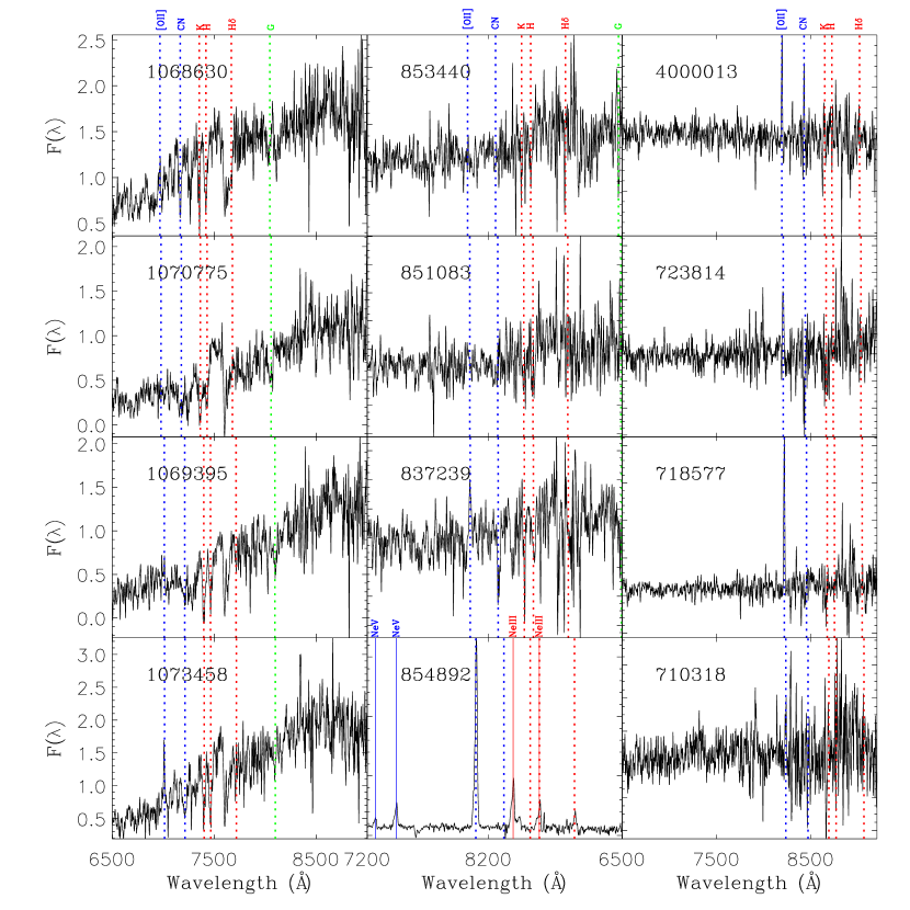
Figure 1.— Sample spectra of confirmed cluster members with Q=0. Left column shows members of cluster SpARCS J161315+564930; center column shows members of SpARCS J161641+554513; right column shows members of SpARCS J161037+552417. Fluxes are in relative units, smoothed by 7 pixels (1 pix $\sim 2$ Å). Prominent spectral features are indicated as vertical-dashed lines. The lowest panel in the center column shows the only confirmed AGN cluster member, discovered in cluster SpARCS J161641+554513 (object 854892). The solid blue vertical lines indicates NeV emission lines while the solid red vertical lines indicate NeIII emission lines. Object 854892 also shows prominent [OII]($\lambda$3727) emission and high-order balmer lines (H$\delta$, H$\epsilon$ and H6) in emission.

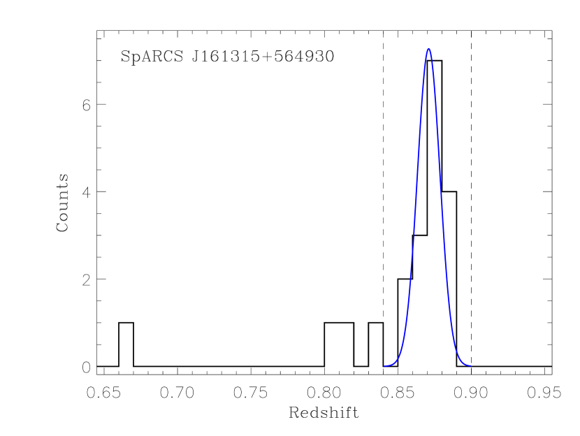
Figure 2.— Left: Squares indicate galaxies with a high-confidence redshift (Quality flag $Q=0$), which were identified by the shifting-gap technique as members of cluster SpARCS J161315+564930. Each galaxy velocity relative to the mean cluster velocity, is plotted as a function of clustercentric distance. Right: Histogram of spectroscopic redshifts in the SpARCS J161315+564930 field-of-view (see Table 2). Confirmed members are within the redshift range $0.84<z<0.90$ indicated by the dashed vertical lines. The blue solid line overlaid is a Gaussian with an rms of 1230 km s^-1 (see Section 4.1).

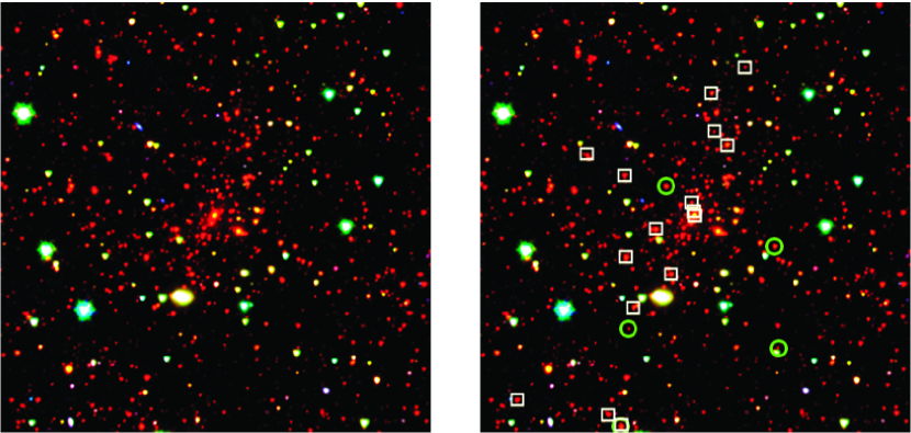
Figure 3.— $r^{\prime}z^{\prime}[3.6]$ color composites of SpARCS J161315+564930 are shown in both panels. The FOV is $7\arcmin$ (3.2 Mpc at the cluster redshift). The white squares (green circles) overlaid on the right panel show the 16 $Q=0$ or $Q=1$ cluster members (and five foreground/background galaxies within the FOV) with spectroscopically-confirmed redshifts from Keck/LRIS (Table 2).

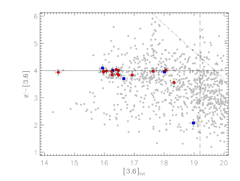
Figure 4.— $z^{\prime}-[3.6]$ vs. $z^{\prime}$ color-magnitude diagram for SpARCS J161315+564930 for galaxies (gray circles) which lie within a projected distance of $R\leq R_{200}$ ($=1.9$ Mpc) of the fiducial cluster center (see Table 1). $R_{200}$ roughly corresponds to the virial radius of the cluster. The colored symbols indicate galaxies with spectroscopic redshifts. Cluster members ($Q=0$ or $Q=1$) are shown by red circles and foreground/background galaxies by blue squares. The three galaxies in Table 2, for which a color could not be determined, do not appear in this figure. The solid line shows the predicted color of an early type galaxy at $z=0.87$ assuming a solar metallicity single burst model with formation redshift $z_{f}=4$. See §5 for a discussion. The vertical dashed line indicates the 5$-\sigma$ limit of 19.2 Vega in the 3.6 $\mu$m-band while the dot-dashed line indicates the color limit taking into account a 5$-\sigma$ limit in the $z^{\prime}$-band of 23.7 Vega.

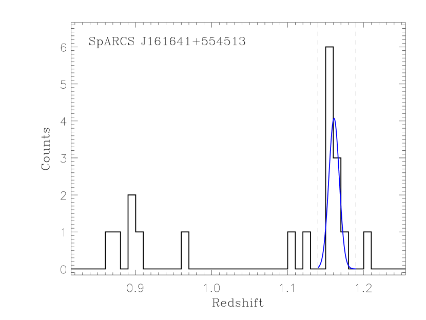
Figure 5.— Left: As for Figure 2, but for the seven Q=0 galaxies identified by the shifting-gap technique as members of cluster SpARCS J161641+554513 (Table 3). Right: As for Figure 2, but for the spectroscopically confirmed galaxies in the FOV of SpARCS J161641+554513. Confirmed members are within the redshift range $1.14<z<1.19$ indicated by the dashed vertical lines.The blue solid line overlaid is a Gaussian with an rms of 950 km s^-1 .

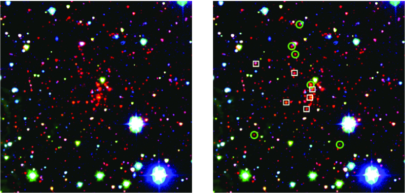
Figure 6.— As for Figure 3, but for SpARCS J161641+554513. The FOV is $5\arcmin$ (2.4 Mpc at the cluster redshift). The white squares (green circles) overlaid on the right panel show the cluster members (foreground/background galaxies) within the FOV (Table 3). See Section 4.2 for a discussion.

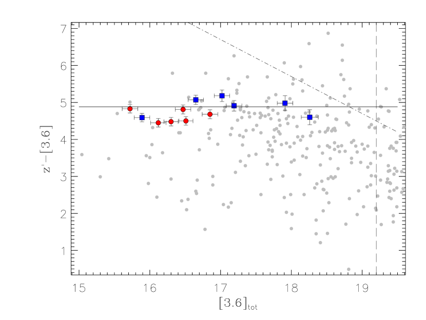
Figure 7.— As for Figure 4 but for SpARCS J161641+554513, for galaxies which lie within a projected distance of $R\leq R_{200}$ ($=1.2$ Mpc) of the fiducial cluster center (see Table 1). Galaxies in Table 3, which lie at $R>R_{200}$, or for which a color could not be determined, do not appear in this figure. See Section 4.2 for more details. The solid line shows the predicted color of an early type galaxy at $z=1.16$ assuming a solar metallicity single burst model with formation redshift $z_{f}=4$. See §5 for a discussion. The vertical dashed line indicates the 5$-\sigma$ limit of 19.2 Vega in the 3.6 $\mu$m-band while the dot-dashed line indicates the color limit taking into account a 5$-\sigma$ limit in the $z^{\prime}$-band of 23.7 Vega.

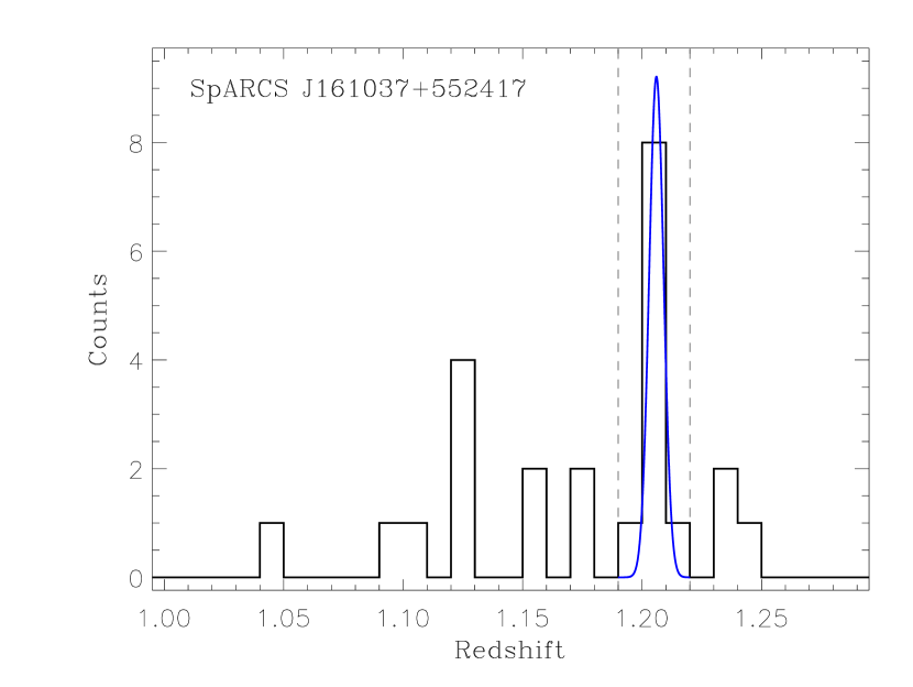
Figure 8.— Left: As for Figure 2 but for the seven Q=0 galaxies identified by the shifting-gap technique as members of cluster SpARCS J161037+552417 (Table 4). Two galaxies, shown by crosses (ID $\#$’s 727869 and 734082 in Table 4) were identified as near-field interlopers. Right: As for Figure 2 but for the spectroscopically confirmed galaxies in the FOV of SpARCS J161037+552417. Confirmed members are within the redshift range $1.19<z<1.22$ indicated by the dashed vertical lines. The blue solid line overlaid is a Gaussian with an rms of 410 km s^-1.

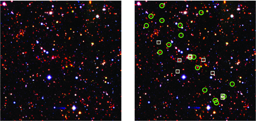
Figure 9.— As for Figure 3, but for SpARCS J161037+552417. The FOV is 6′(2.9 Mpc at the cluster redshift). The white squares (green circles) overlaid on the right panel show the cluster members (foreground/background galaxies) within the FOV (Table 4). See Section 4.3 for a discussion.

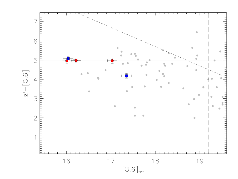
Figure 10.— As for Figure 4, but for SpARCS J161037+552417 for galaxies at $R\leq R_{200}$ ($=510$ kpc) of the fiducial cluster center (see Table 1). Galaxies in Table 4, at $R>R_{200}$, or for which a color could not be determined, do not appear in this figure. The three clusters members (red circles) correspond to galaxies with ID $\#$’s 723814, 722784, and 722712 in Table 4. See Section 4.3 for more details. The solid line shows the predicted color of an early type galaxy at $z=1.210$ assuming a solar metallicity single burst model with formation redshift $z_{f}=4$. See §5 for a discussion. The vertical dashed line indicates the 5$-\sigma$ limit of 19.2 Vega in the 3.6 $\mu$m-band while the dot-dashed line indicates the color limit taking into account a 5$-\sigma$ limit in the $z^{\prime}$-band of 23.7 Vega.

Figure 11.— Left: $z^{\prime}-[3.6]$ color vs. spectroscopic redshift for the six SpARCS clusters confirmed to date (Table 5). Solid, dotted and and dashed lines show color as a function of redshift for solar metallicity single burst BC03 models with formation redshifts of $z_{f}=3$, 4 and 10. See §5.1 for a discussion. Right: Richness mass vs. dynamical mass estimates (see Table 5). $M_{200}^{Bgc}$ is estimated from the $B_{gc}$ richness parameter (§5.2), and $M_{200}^{\sigma}$ is estimated from the velocity dispersion (§4.1 and Table 1).

References

- Andreon et al. (2009) Andreon, S., Maughan, B., Trinchieri, G., & Kurk, J. 2008, A&A, 507, 147
- Becker et al. (2007) Becker, M. R., et al. 2007, ApJ, 669, 905
- Beers et al. (1990) Beers, T. C., Flynn, K., & Gebhardt, K. 1990, AJ, 100, 32
- Bertin & Arnouts (1996) Bertin, E., & Arnouts, S. 1996, A&AS, 117, 393
- Blindert (2006) Blindert, K. 2006, Ph.D. Thesis, University of Toronto, Canada
- Bremer et al. (2006) Bremer, M. N., et al. 2006, MNRAS, 371, 1427
- Brodwin et al. (2006) Brodwin, M., et al. 2006, ApJ, 651, 791
- Bruzual & Charlot (2003) Bruzual, G., & Charlot, S. 2003, MNRAS, 344, 1000
- Carlstrom et al. (2009) Carlstrom, J. E., et al. 2009, arXiv:0907.4445
- Demarco et al. (2005) Demarco, R., et al. 2005, A&A, 432, 381
- Demarco et al. (2007) Demarco, R., et al. 2007, ApJ, 663, 164
- Dobbs et al. (2006) Dobbs, M., et al. 2006, New Astronomy Review, 50, 960
- Eisenhardt et al. (2008) Eisenhardt, P. R. M., et al. 2008, ApJ, 684, 905
- Fadda et al. (1996) Fadda, D., Girardi, M., Giuricin, G., Mardirossian, F., & Mezzetti, M. 1996, ApJ, 473, 670
- Fazio et al. (2004) Fazio, G. G., et al. 2004, ApJS, 154, 10
- Gilbank et al. (2007) Gilbank, D. G., Yee, H. K. C., Ellingson, E., Gladders, M. D., Barrientos, L. F., & Blindert, K. 2007, AJ, 134, 282
- Gioia et al. (2004) Gioia, I. M., Braito, V., Branchesi, M., Della Ceca, R., Maccacaro, T., & Tran, K.-V. 2004, A&A, 419, 517
- Girardi et al. (1993) Girardi, M., Biviano, A., Giuricin, G., Mardirossian, F., & Mezzetti, M. 1993, ApJ, 404, 38
- Girardi et al. (2005) Girardi, M., Demarco, R., Rosati, P., & Borgani, S. 2005, A&A, 442, 29
- Gladders et al. (2007) Gladders, M. D., Yee, H. K. C., Majumdar, S., Barrientos, L. F., Hoekstra, H., Hall, P. B., & Infante, L. 2007, ApJ, 655, 128
- Gladders & Yee (2000) Gladders, M. D., & Yee, H. K. C. 2000, AJ, 120, 2148
- Gladders & Yee (2005) Gladders, M. D., & Yee, H. K. C. 2005, ApJS, 157, 1
- Goto et al. (2008) Goto, T., et al. 2008, PASJ, 60, 531
- Hoekstra et al. (2000) Hoekstra, H., Franx, M., & Kuijken, K. 2000, ApJ, 532, 88
- Jee et al. (2005) Jee, M. J., White, R. L., Ford, H. C., Blakeslee, J. P., Illingworth, G. D., Coe, D. A., & Tran, K.-V. H. 2005, ApJ, 634, 813
- Kinney et al. (1996) Kinney, A. L., Calzetti, D., Bohlin, R. C., McQuade, K., Storchi-Bergmann, T., & Schmitt, H. R. 1996, ApJ, 467, 38
- Koester et al. (2007) Koester, B. P., et al. 2007, ApJ, 660, 239
- Kosowsky (2003) Kosowsky, A. 2003, New Astronomy Review, 47, 939
- Koyama et al. (2007) Koyama, Y., Kodama, T., Tanaka, M., Shimasaku, K., & Okamura, S. 2007, MNRAS, 382, 1719
- Krick et al. (2008) Krick, J. E., Surace, J. A., Thompson, D., Ashby, M. L. N., Hora, J. L., Gorjian, V., & Yan, L. 2008, ApJ, 686, 918
- Kurk et al. (2008) Kurk, J., et al. 2008, Astronomical Society of the Pacific Conference Series, 399, 332
- Kurtz et al. (1992) Kurtz, M. J., Mink, D. J., Wyatt, W. F., Fabricant, D. G., Torres, G., Kriss, G. A., & Tonry, J. L. 1992, Astronomical Data Analysis Software and Systems I, 25, 432
- Lacy et al. (2005) Lacy, M., et al. 2005, ApJS, 161, 41
- Lawrence et al. (2007) Lawrence, A., et al. 2007, MNRAS, 379, 1599
- Lonsdale et al. (2003) Lonsdale, C. J., et al. 2003, PASP, 115, 897
- McCarthy et al. (1998) McCarthy, J. K., et al. 1998, Proc. SPIE, 3355, 81
- McCarthy et al. (2007) McCarthy, P. J., et al. 2007, ApJ, 664, L17
- Mullis et al. (2005) Mullis, C. R., Rosati, P., Lamer, G., Böhringer, H., Schwope, A., Schuecker, P., & Fassbender, R. 2005, ApJ, 623, L85
- Muzzin et al. (2007) Muzzin, A., Yee, H. K. C., Hall, P. B., & Lin, H. 2007, ApJ, 663, 150
- Muzzin et al. (2008) Muzzin, A., Wilson, G., Lacy, M., Yee, H. K. C., & Stanford, S. A. 2008, ApJ, 686, 966
- Muzzin et al. (2009) Muzzin, A., et al. 2009, ApJ, 698, 1943
- Oke (1990) Oke, J. B. 1990, AJ, 99, 1621
- Oke et al. (1995) Oke, J. B., et al. 1995, PASP, 107, 375
- Rosati et al. (1999) Rosati, P., Stanford, S. A., Eisenhardt, P. R., Elston, R., Spinrad, H., Stern, D., & Dey, A. 1999, AJ, 118, 76
- Rosati et al. (2004) Rosati, P., et al. 2004, AJ, 127, 230
- Rozo et al. (2009a) Rozo, E., et al. 2009, ApJ, 703, 601
- Rozo et al. (2009b) Rozo, E., et al. 2009, arXiv:0902.3702
- Ruhl et al. (2004) Ruhl, J., et al. 2004, Proc. SPIE, 5498, 11
- Shapley et al. (2003) Shapley, A. E., Steidel, C. C., Pettini, M., & Adelberger, K. L. 2003, ApJ, 588, 65
- Shupe et al. (2008) Shupe, D. L., et al. 2008, AJ, 135, 1050
- Stanford et al. (1997) Stanford, S. A., Elston, R., Eisenhardt, P. R., Spinrad, H., Stern, D., & Dey, A. 1997, AJ, 114, 2232
- Stanford et al. (2002) Stanford, S. A., Holden, B., Rosati, P., Eisenhardt, P. R., Stern, D., Squires, G., & Spinrad, H. 2002, AJ, 123, 619
- Stanford et al. (2005) Stanford, S. A., et al. 2005, ApJ, 634, L129
- Stanford et al. (2006) Stanford, S. A., et al. 2006, ApJ, 646, L13
- Surace et al. (2005) Surace, J., Shupe, D. L., Fang, F., Lonsdale, C. J., & Gonzalez-Solares, E. 2005, SSC website release
- Tran et al. (2007) Tran, K.-V. H., Franx, M., Illingworth, G. D., van Dokkum, P., Kelson, D. D., Blakeslee, J. P., & Postman, M. 2007, ApJ, 661, 750
- Tonry & Davis (1979) Tonry, J., & Davis, M. 1979, AJ, 84, 1511
- van Breukelen et al. (2007) van Breukelen, C., et al. 2007, MNRAS, 382, 971
- Wilson et al. (2009) Wilson, G., et al. 2009, ApJ, 698, 1934
- Yee & Ellingson (2003) Yee, H. K. C., & Ellingson, E. 2003, ApJ, 585, 215
- Yee & López-Cruz (1999) Yee, H. K. C., & López-Cruz, O. 1999, AJ, 117, 1985
- Yee et al. (2007) Yee, H. K. C., Gladders, M. D., Gilbank, D. G., Majumdar, S., Hoekstra, H., Ellingson, E., & the RCS-2 Collaboration 2007, arXiv:astro-ph/0701839
- York et al. (2000) York, D. G., et al. 2000, AJ, 120, 1579
- Zatloukal et al. (2007) Zatloukal, M., Röser, H.-J., Wolf, C., Hippelein, H., & Falter, S. 2007, A&A, 474, L5