Moment-Based Analysis of Synchronization in Small-World Networks of Oscillators

Abstract

In this paper, we investigate synchronization in a small-world network of coupled nonlinear oscillators. This network is constructed by introducing random shortcuts in a nearest-neighbors ring. The local stability of the synchronous state is closely related with the support of the eigenvalue distribution of the Laplacian matrix of the network. We introduce, for the first time, analytical expressions for the first three moments of the eigenvalue distribution of the Laplacian matrix as a function of the probability of shortcuts and the connectivity of the underlying nearest-neighbor coupled ring. We apply these expressions to estimate the spectral support of the Laplacian matrix in order to predict synchronization in small-world networks. We verify the efficiency of our predictions with numerical simulations.

I Introduction

In recent years, systems of dynamical nodes interconnected through a complex network have attracted a good deal of attention [20]. Biological and chemical networks, neural networks, social and economic networks [9], the power grid, the Internet and the World Wide Web [8] are examples of the wide range of applications that motivate this interest (see also [15], [4] and references therein). Several modeling approaches can be found in the literature [8], [22], [1]. In this paper, we focus our attention on the so-called small-world phenomenon and a model proposed by Newman and Strogatz to replicate this phenomenon.

Once the network is modeled, one is usually interested in two types of problems. The first involves structural properties of the model. The second involves the performance of dynamical processes run on those networks. In the latter direction, the performance of random walks [12], Markov processes [6], gossip algorithms [5], consensus in a network of agents [16], [10], or synchronization of oscillators [21], [17], are very well reported in the literature. These dynamical processes are mostly studied in the traditional context of deterministic networks of relatively small size and/or regular structure. Even though many noteworthy results have been achieved for large-scale probabilistic networks [13]–[2], there is substantial reliance on numerical simulations.

The eigenvalue spectrum of an undirected graph contains a great deal of information about structural and dynamical properties [7]. In particular, we focus our attention on the spectrum of the (combinatorial) Laplacian matrix uniquely associated with an undirected graph [3]. This spectrum contains useful information about, for example, the number of spanning trees, or the stability of synchronization of a network of oscillators. We analyze the low-order moments of the Kirchhoff matrix spectrum corresponding to small-world networks.

The paper is organized as follows. In Section II, we review the master stability function approach. In Section III, we derive closed-form expressions for the low-order moments of the Laplacian eigenvalue distribution associated with a probabilistic small-world network. Our expressions are valid for networks of asymptotically large size. Section IV applies our results to the problem of synchronization of a probabilistic small-world network of oscillators. The numerical results in this section corroborate our predictions.

II Synchronization of Nonlinear Oscillators

In this section we review the master-stability-function (MSF) approach, proposed by Pecora and Carrol in [17], to study local stability of synchronization in networks of nonlinear oscillators. Using this approach, we reduce the problem of studying local stability of synchronization to the algebraic problem of studying the spectral support of the Laplacian matrix of the network. First, we introduce some needed graph-theoretical background.

II-A Spectral Graph Theory Background

In the case of a network with symmetrical connections, undirected graphs provide a proper description of the network topology. An undirected graph $G$ consists of a set of $N$ nodes or vertices, denoted by $V=\left\{v_{1},...,v_{n}\right\}$, and a set of edges $E$, where $E\in V\times V$. In our case, $\left(v_{i},v_{j}\right)\in E$ implies $\left(v_{j},v_{i}\right)\in E,$ and this pair corresponds to a single edge with no direction; the vertices $v_{i}$ and $v_{j}$ are called adjacent vertices (denoted by $v_{i}\sim v_{j}$) and are incident to the edge $\left(v_{i},v_{j}\right)$. We only consider simple graphs (i.e., undirected graphs that have no self-loops, so $v_{i}\neq v_{j}$ for an edge $\left(v_{i},v_{j}\right)$, and no more than one edge between any two different vertices). A walk on $G$ of length $k$ from $v_{0}$ to $v_{k}$ is an ordered set of vertices $\left(v_{0},v_{1},...,v_{k}\right)$ such that $\left(v_{i},v_{i+1}\right)\in E,$ for $i=0,1,...,k-1$; if $\nu_{k}=\nu_{0}$ the walk is said to be closed.

The degree $d_{i}$ of a vertex $v_{i}$ is the number of edges incident to it. The degree sequence of $G$ is the list of degrees, usually given in non-increasing order. The clustering coefficient, introduced in [22], is a measure of the number of triangles in a given graph, where a triangle is defined by the set of edges $\left\{\left(i,j\right),\left(j,k\right),\left(k,i\right)\right\}$ such that $i\sim j\sim k\sim i$. Specifically, we define clustering as the total number of triangles in a graph, $T\left(G\right),$ divided by the number of triangles in a complete (all-to-all) graph with $N$ vertices, i.e., the coefficient is equal to $T\left(G\right)\left/\binom{N}{3}\right..$

It is often convenient to represent graphs via matrices. There are several choices for such a representation. For example, the adjacency matrix of an undirected graph $G,$ denoted by $A(G)=[a_{ij}]$, is defined entry-wise by $a_{ij}=1$ if nodes $i$ and $j$ are adjacent, and $a_{ij}=0$ otherwise. (Note that $a_{ii}=0$ for simple graphs.) Notice also that the degree $d_{i}$ can be written as $d_{i}=\sum_{j=1}^{N}a_{ij}$. We can arrange the degrees on the diagonal of a diagonal matrix to yield the degree matrix, $D=diag\left(d_{i}\right)$. The Laplacian matrix (also called Kirchhoff matrix, or combinatorial Laplacian matrix) is defined in terms of the degree and adjacency matrices as $L(G)=D(G)-A(G).$ For undirected graphs, $L(G)$ is a symmetric positive semidefinite matrix [3]. Consequently, it has a full set of $N$ real and orthogonal eigenvectors with real non-negative eigenvalues. Since all rows of $L$ sum to zero, it always admits a trivial eigenvalue $\lambda_{1}=0$, with corresponding eigenvector $\mathbf{v}_{1}=\left(1,1,...,1\right)^{T}$.

The moments of the Laplacian eigenvalue spectrum are central to our paper. Denote the eigenvalues of our $N\times N$ symmetric Laplacian matrix $L(G)$ by $0=\lambda_{1}\left(G\right)\leq...\leq\lambda_{N}\left(G\right)$. The empirical spectral density (ESD) of $L(G)$ is defined as

$$\mu_{G}\left(\lambda\right)=\frac{1}{N}\sum_{i=1}^{N}\delta\left(\lambda-\lambda_{i}\right),$$

where $\delta(\cdot)$ is the Dirac delta function. The $k$-th order moment of the ESD of $L(G)$ is defined as:

$$q_{k}(G)=\frac{1}{N}\sum_{i=1}^{N}\lambda_{i}(G)^{k}$$

(which is also called the $k$-th order spectral moment).

In the following subsection, we illustrate how a network of identical nonlinear oscillators synchronizes whenever the Laplacian spectrum is contained in a certain region on the real line. This region of synchronization is exclusively defined by the dynamics of each isolated oscillator and the type of coupling [17], [11]. This simplifies the problem of synchronization to the problem of locating the Laplacian eigenvalue spectrum.

II-B Synchronization as a Spectral Graph Problem

Several techniques have been proposed to analyze the synchronization of coupled identical oscillators. In [23], well-known results in control theory, such as the passivity criterion, the circle criterion, and a result on observer design are used to derive synchronization criteria for an array of identical nonlinear systems. In [19], the authors use contraction theory to derive sufficient conditions for global synchronization in a network of nonlinear oscillators. We pay special attention to the master-stability-function (MSF) approach, [17]. This approach provides us with a criterion for local stability of synchronization based on the numerical computation of Lyapunov exponents. Even though quite different in nature, the mentioned techniques emphasize the key role played by the graph eigenvalue spectrum.

In this paper we consider a time-invariant network of $N$ identical oscillators, one located at each node, linked with ‘diffusive’ coupling. The state equations modeling the dynamics of the network are

$$\mathbf{\dot{x}}_{i}=\mathbf{f}\left(\mathbf{x}_{i}\right)+\gamma\sum_{j=1}^{N}a_{ij}\Gamma\left(\mathbf{x}_{j}-\mathbf{x}_{i}\right),\text{ }i=1,...,N$$ (1)

where $\mathbf{x}_{i}$ represents an $n$-dimensional state vector corresponding to the $i$-th oscillator. The nonlinear function $\mathbf{f}\left(\cdot\right)$ describes the (identical) dynamics of the isolated nodes. The positive scalar $\gamma$ can be interpreted as a global coupling strength parameter. The $n\times n$ matrix $\Gamma$ represents how states in neighboring oscillators couple linearly, and $a_{ij}$ are the entries of the adjacency matrix. By simple algebraic manipulations, one can write down Eq. (1) in terms of the Laplacian entries, $L(G)=\left[l_{ij}\right]$, as

$$\mathbf{\dot{x}}_{i}=\mathbf{f}\left(\mathbf{x}_{i}\right)-\gamma\sum_{j=1}^{N}l_{ij}\Gamma\mathbf{x}_{j}\text{, for }i=1,...,N.$$ (2)

We say that the network of oscillators is at a synchronous equilibrium if $\mathbf{x}_{1}(t)=\mathbf{x}_{2}(t)=...=\mathbf{x}_{N}(t)=\mathbf{\phi}\left(t\right)$, where $\mathbf{\phi}\left(t\right)$ represents a solution for $\mathbf{\dot{x}}=\mathbf{f}\left(\mathbf{x}\right)$. In [17], the authors studied the local stability of the synchronous equilibrium. Specifically, they considered a sufficiently small perturbation, denoted by $\mathbf{\varepsilon}_{i}(t)$, from the synchronous equilibrium, i.e.,

$$\mathbf{x}_{i}(t)=\mathbf{\phi}\left(t\right)+\mathbf{\varepsilon}_{i}(t).$$

After appropriate linearization, one can derive the following equations to approximately describe the evolution of the perturbations:

$$\mathbf{\dot{\varepsilon}}_{i}=\mathbf{Df}\left(t\right)\,\mathbf{\varepsilon}_{i}(t)-\gamma\sum_{j=1}^{n}l_{i,j}\Gamma\,\mathbf{\varepsilon}_{j}(t)\text{, for }i=1,...,N.$$ (3)

where $\mathbf{Df}\left(t\right)$ is the Jacobian of $\mathbf{f}\left(\cdot\right)$ evaluated along the trajectory $\mathbf{\phi}\left(t\right)$. This Jacobian is an $n\times n$ matrix with time-variant entries. Following the methodology introduced in [17], Eq. (3) can be similarity transformed into a set of linear time-variant (LTV) ODEs of the form:

$$\mathbf{\dot{\xi}}_{i}\mathbf{=}\left[\mathbf{Df}\left(t\right)+(\gamma\lambda_{i}\left(G\right))~{}\Gamma\right]\mathbf{\xi}_{i},\text{ for }i=1,...,N,$$ (4)

where $\{\lambda_{i}\left(G\right)\}_{1\leq i\leq N}$ is the set of eigenvalues of $L\left(G\right)$. Based on the stability analysis presented in [17], the network of oscillators in (1) presents a locally stable synchronous equilibrium if the corresponding maximal nontrivial Lyapunov exponents of (4) is negative for $i=2,...,N$.

Inspired in Eq. (4), Pecora and Carroll studied in [17] the stability of the following parametric LTV-ODE in the parameter $\sigma$:

$$\mathbf{\dot{\xi}=}\left[\mathbf{Df}\left(t\right)+\sigma\Gamma\right]\mathbf{\xi,}$$ (5)

where $\mathbf{Df}\left(t\right)$ is the linear time-variant Jacobian in Eq. (3). The master stability function (MSF), denoted by $F\left(\sigma\right)$, is defined as the value of the maximal nontrivial Lyapunov exponent of (5) as a function of $\sigma$. Note that $F\left(\sigma\right)$ depends exclusively on $\mathbf{f}\left(\cdot\right)$ and $\Gamma$, and is independent of the coupling topology, i.e., independent of $L\left(G\right)$. The region of synchronization is, therefore, defined by the range of $\sigma>0$ for which $F\left(\sigma\right)<0$. For a broad class of systems, the MSF is negative in the interval $\sigma\in\left[0,\sigma_{\max}\right]\equiv S$ (although more generic stability sets are also possible, we assume, for simplicity, this is the case in subsequent derivations). In order to achieve synchronization, the set of scaled nontrivial Laplacian eigenvalues, $\{\gamma\lambda_{i}\}_{2\leq i\leq N}$, must be located inside the region of synchronization, $S$. This condition is equivalent to: $\gamma\lambda_{2}>0$ and $\gamma\lambda_{N}<\sigma_{\max}$.

We illustrate how to use of the above methodology in the following example:

Example 1

Study the stability of synchronization of a ring of 6 coupled Rössler oscillators [14]. The dynamics of each oscillator is described by the following system of three nonlinear differential equations:

$$\dot{x}_{i} = -\left(y_{i}+z_{i}\right),$$

$$\dot{y}_{i} = x_{i}+a\,y_{i},$$

$$\dot{z}_{i} = b+z_{i}\left(x_{i}-c\right).$$

The adjacency entries, $a_{ij}$, of a ring graph of six nodes are $a_{i,j}=1$ if $j\in\{(i+1)\text{ mod }6,(i-1)\text{ mod }6\}$, for $i=1,2,...,6$, and $a_{ij}=0$ otherwise. The dynamics of this ring of oscillators are defined by:

$$\left[\begin{array}[]{c}\dot{x}_{i}\\ \dot{y}_{i}\\ \dot{z}_{i}\end{array}\right]=\left[\begin{array}[]{c}-\left(y_{i}+z_{i}\right)\\ x_{i}+a\,y_{i}\\ b+z_{i}\left(x_{i}-c\right)\end{array}\right]+\gamma\sum_{j\in R\left(i\right)}\left[\begin{array}[]{c}x_{j}-x_{i}\\ 0\\ 0\end{array}\right]$$ (6)

where  we have chosen to connect the oscillators through their $x_{i}$ states exclusively. Our choice is reflected in the structure of the $3\times 3$ matrix, $\Gamma$, inside the summation in Eqn. (6).

Numerical simulations of an isolated Rössler oscillator unveil the existence of a periodic trajectory with period $T=5.749$ when the parameters in Eqn. (6) take the values $a=0.2,\,b=0.2,$ and $c=2.5$ (see Fig. 1). We denote this periodic trajectory by $\mathbf{\phi}\left(t\right)=\left[\phi_{x}\left(t\right),\phi_{y}\left(t\right),\phi_{z}\left(t\right)\right]$. In our specific case, the LTP differential equation (5) takes the following form:

$$\mathbf{\dot{\xi}}=\left(\left[\begin{array}[]{ccc}0&-1&-1\\ 1&a&0\\ \phi_{z}\left(t\right)&0&c\end{array}\right]+\sigma\left[\begin{array}[]{ccc}1&0&0\\ 0&0&0\\ 0&0&0\end{array}\right]\right)\mathbf{\xi,}$$ (7)

where the leftmost matrix in the above equation represents the Jacobian of the isolated Rössler evaluated along the periodic trajectory $\mathbf{\phi}\left(t\right),$ and the rightmost matrix represents $\Gamma$.

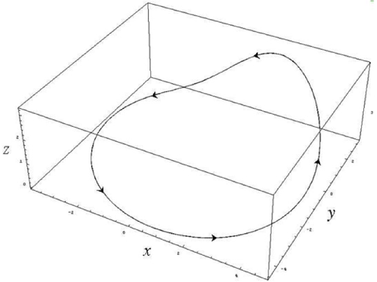
Figure 1: Periodic trajectory with period $T=5.749$ in a Rössler oscillator when the parameters in Eqn. (6) take the values $a=0.2,\,b=0.2,$ and $c=2.5$.

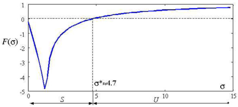
Figure 2: Numerical values of the maximum Floquet exponent of Eqn. (7) for $\sigma\in\left[0,15\right]$, discretizing at intervals of length $0.2$.

In Fig. 2, we plot the numerical values of the maximum Floquet exponent of Eqn. (7) for $\sigma\in\left[0,15\right]$, discretizing at intervals of length $0.2$. This plot shows the range in which the maximal Floquet exponent is negative. This range of stability is $S=\left(0,\sigma^{\ast}\right)$, for $\sigma^{\ast}\approx 4.7$. The MSF criterion introduced in [17] states that the synchronous equilibrium is locally stable if the set of values $\{\gamma~{}\lambda_{i}\left(G\right)\}_{i=2,...,n}$ lies inside the stability range, $S$. For the case of a 6-ring configuration, the eigenvalues of $L\left(G\right)$ are $\left\{{0,1,1,3,3,4}\right\}$, so the set $\{\gamma\lambda_{i}\}_{i=2,...,n}$ is $\left\{\gamma,\gamma,3\gamma,3\gamma,4\gamma\right\}.$ Therefore, we achieve stability for $\gamma\in(0,\sigma^{\ast}/\lambda_{n}\left(G\right))$, where in our case $\sigma^{\ast}/\lambda_{n}\left(G\right)\approx 1.175$.

We now illustrate this result with several numerical simulations. First, we plot in Fig. 3.a the temporal evolution of the $x_{i}$ states of the 6-ring when $\gamma=1.0$. Observe how, since $\gamma\in\left(0,1.175\right)$, we achieve asymptotic synchronization. On the other hand, if we choose $\gamma=1.3\notin\left(0,1.175\right)$, the time evolution of the set of oscillators does not converge to a common trajectory (see Fig. 3.b); instead, the even and odd nodes settle into two different trajectories.

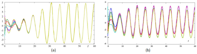
Figure 3: In Fig. a, we plot the temporal evolution of the $x_{i}$ states of the 6-ring when $\gamma=1.0$. In Fig.b, we plot the time evolution of the set of oscillators for $\gamma=1.3\notin\left(0,1.175\right)$.

In the next subsection, we propose an approach to estimating the support of the eigenvalue distribution of large-scale probabilistic networks from low-order spectral moments. This allows us to predict synchronization in a large-scale Chung-Lu network.

III Spectral Analysis of Small-World Networks

In this section we study the Laplacian eigenvalue spectrum of a variant of Watts-Strogatz small-world network [22]. After describing the model, we use algebraic graph theory to compute explicit expressions for the Laplacian moments of a small-world network as a function of its parameters. Our derivations are based on a probabilistic analysis of the expected spectral moments of the Laplacian for asymptotically large small-world networks.

III-A Small-World Probabilistic Model

We consider a one-dimensional lattice of $N$ vertices, $\left\{v_{1},...,v_{N}\right\}$, with periodic boundary conditions, i.e., on a ring, and connect each vertex $v_{i}$ to its $2k$ closest neighbors, i.e., $v_{i}$ is connected to the set of nodes $\left\{v_{j}:j\in\left[\left(i-k\right)\text{mod}N,\left(i+k\right)\text{mod}N\right]\right\}$. Then, instead of rewiring a fraction of the edges in the regular lattice as proposed by Watts and Strogatz [22], we add some random ‘shortcuts’ to the one-dimensional lattice. These shortcuts are added by independently assigning edges between each pair of nodes $\left(i,j\right),$ $1\leq i<j\leq N$ with probability $p$. The resulting small-world graph is intermediate between a regular lattice (achieved for $p=0$) and a classical random graph (achieved for $p=1$). In general, small-world networks share properties with both the regular grid and the classical random graph for $0<p<1$. In particular, they show the following apparently contradictory features:

(i) most nodes are not neighbors of one another (such as in a regular grid), and

(ii) most nodes can be reached from every other node by a small number of steps (such as in a random graph).

An interesting property observed in this model was the following: for small probability of rewiring, $p\ll 1$, the number of triangles in the network is nearly the same as that of the regular lattice, but the average shortest-path length is close to that of classical random graphs. In the rest of the paper we assume we are in the range of $p$ in which this property holds, in particular, we will prescribe $p$ to be  $r/N$, for a given parameter $r$.

In the coming sections we shall study spectral properties of the Laplacian matrix associated to the above small-world model. In our derivations we will need the probabilistic distribution for the degrees. It is well known that, for asymptotically large graphs, the degree distribution of a classical random graph with average degree $r$ is a Poisson distribution with rate $r$. Hence, the degree distribution of the above small-world network is

$$\Pr(d_{i}=d)=\left\{\begin{array}[]{ll}0,&\text{for }d<2k,\\ \frac{r^{d-2k}e^{-r}}{(d-2k)!},&\text{for }d\geq 2k,\end{array}\right.$$ (8)

which corresponds to a Poisson with parameter $r$ ‘shifted’ $2k$ units. The Poisson distribution is shifted to take into account the degree of the regular $2k$-neighbors ring superposed to the random shortcuts.

Furthermore, it is well known that the clustering coefficient (or, equivalently, the number of triangles) of the regular $2k$-neighbors rings is very lightly perturbed by the addition of random shortcuts for $p=r/N$. In particular, one can prove the following result:

$$\mathbb{E}[T]=(1+o(1))\,\frac{1}{3}N\binom{2k}{2},$$ (9)

where the dominant term, $\frac{1}{3}N\binom{2k}{2}$, corresponds to the exact number of triangles in a $2k$-neighbors ring with $N$ nodes.

In the following section, we shall derive explicit expressions for the first low-order spectral moments of the Laplacian matrix associated with the small-world model herein described. Even though our analysis is far from complete, in that only low-order moments are provided, valuable information regarding spectral properties can be retrieved from our results.

III-B Algebraic Analysis of Spectral Moments

In this section we deduce closed-form expressions for the first three moments of the Laplacian spectrum of any simple graph $G$. First, we express the spectral moments as a trace using the following identity:

$$q_{k}\left(G\right)=\frac{1}{N}\sum_{i=1}^{N}\lambda_{i}\left(G\right)^{k}=\frac{1}{N}\,\text{tr}\,L\left(G\right)^{k}.$$ (10)

This identity is derived from the fact that trace is conserved under diagonalization (in general, under any similarity transformation). In the case of the first spectral moment, we obtain

$$q_{1}=\frac{1}{N}\text{tr}\left(D-A\right)=\frac{1}{N}\sum_{i=1}^{N}d_{i}.$$

where $\overline{d}$ is the average degree of the graph. For analytical and numerical reasons, we define the normalized Kirchhoff moment as

$$\overline{q}_{k}=\frac{1}{N}\sum_{i=1}^{N}\left(\lambda_{i}/\overline{d}\right)^{k}=\frac{1}{N\,\overline{d}^{k}}\,\text{tr}\left(D-A\right)^{k}.$$ (11)

The fact that $D$ and $A$ do not commute forecloses the possibility of using Newton’s binomial expansion on $\left(D-A\right)^{k}$. On the other hand, the trace operator allows us to cyclically permute multiplicative chains of matrices. For example, tr$\,\left(AAD\right)=$tr$\,\left(ADA\right)=$tr$\,\left(DAA\right)$. Thus, for words of length $k\leq 3$, one can cyclically arrange all binary words in the expansion of (11) into the standard binomial expression:

$$\overline{q}_{k}=\sum_{\alpha=0}^{k}\binom{k}{\alpha}\frac{(-1)^{\alpha}}{\overline{d}^{k}N}\text{tr\thinspace}\left(A^{\alpha}D^{k-\alpha}\right)\text{,\quad\quad for }k\leq 3.$$ (12)

Also, we can make use of the identity tr$\left(A^{\alpha}D^{k-\alpha}\right)=\sum_{i=1}^{N}\left(A^{\alpha}\right)_{ii}d_{i}^{k-\alpha}$ to write

$$\overline{q}_{k}=\sum_{\alpha=0}^{k}\sum_{i=1}^{N}\binom{k}{\alpha}\frac{(-1)^{\alpha}}{\overline{d}^{k}N}d_{i}^{k-\alpha}\left(A^{\alpha}\right)_{ii}\text{,\quad\quad for }k\leq 3.$$ (13)

Note that this expression is not valid for $k\geq 4$. For example, for $k=4$, we have that tr$\left(AADD\right)\neq$tr$\left(DADA\right).$

We now analyze each summand in expression (13) from a graph-theoretical point of view. Specifically, we find a closed-form solution for each term tr$\left(A^{i}D^{j}\right)$, for all pairs $1\leq i+j\leq 3$, as a function of the degree sequence and the number of triangles in the network. In our analysis, we make use of the following results from [3]:

Lemma 2

The number of closed walks of length $\alpha$ in a graph $G$, joining node $i$ to itself, is given by the $i$-th diagonal entry of the matrix $A^{\alpha}$.

Corollary 3

Let $G$ be a simple graph. Denote by $t_{i}$ the number of triangles touching node $i$. Then,

$$\left(A\right)_{ii}=0,\text{ }\left(A^{2}\right)_{ii}=d_{i},\text{ and }\left(A^{3}\right)_{ii}=2\,t_{i}.$$ (14)

After substituting (14) into (13), and straightforward algebraic simplifications, we obtain the following exact expression for the low-order normalized spectral moments of a given Kirchhoff matrix $K$:

$$\overline{q}_{k}=\left\{\begin{array}[]{lc}1,&\text{for }k=1,\\ \frac{1}{N\,\overline{d}^{2}}\left(\sum_{i=1}^{N}d_{i}^{2}+\sum_{i=1}^{N}d_{i}\right),&\text{for }k=2,\\ \frac{1}{N\,\overline{d}^{3}}\left[\left(\sum_{i=1}^{N}\,d_{i}^{3}+3\sum_{i=1}^{N}d_{i}^{2}\right)-6\,T\right],&\text{for }k=3,\end{array}\right.$$ (15)

where $T=\frac{1}{3}\sum_{i=1}^{N}t_{i}$ is the total number of triangles in the network.

It is worth noting how our spectral results are written in terms of two widely reported measurements, [15]: the degree sequence and the clustering coefficient (which provides us with the total number of triangles.) This allows us to compute low-order spectral moments of many real-world networks without performing an explicit eigenvalue decomposition.

III-C Probabilistic Analysis of Spectral Moments

In this section, we use Eq. (15) to compute the first three expected Laplacian moments of the small-world model under consideration. The expected moments can be computed if we had explicit expressions for the moments of the degrees, $\mathbb{E}[d_{i}]$, $\mathbb{E}[d_{i}^{2}]$,  and $\mathbb{E}[d_{i}^{3}]$, and the expected number of triangles, $\mathbb{E}[T]$. Since we know the degree distribution (8) for this model, the moments of the degrees can be computed to be:

$$\mathbb{E}[d_{i}] = r+2k,$$ (16)

$$\mathbb{E}[d_{i}^{2}] = r^{2}+\left(1+4k\right)\,r+4k^{2},$$

$$\mathbb{E}[d_{i}^{3}] = r^{3}+15\left(3+6k\right)\,r^{2}+\left(1+6k+12k^{2}\right)~{}r-8k^{3}.$$

We can therefore substitute the expressions (9) and (16) in Eq. (15) in order to derive the following expressions for the (non-normalized) expected Laplacian moments for $N\rightarrow\infty$:

$$\mathbb{E}[q_{1}] \rightarrow \,r+2k,$$ (17)

$$\mathbb{E}[q_{2}] \rightarrow \,r^{2}+\left(4k+2\right)\,r+4k^{2}+2k,$$

$$\mathbb{E}[q_{3}] \rightarrow r^{3}+\left(6k+6\right)\,r^{2}+\left(12k^{2}+18k+4\right)\,r$$

$$+8k^{2}+8k^{3}+2k.$$

In the following table we compare the numerical values of the Laplacian moments corresponding to one random realization of the model under consideration with the analytical predictions in (17). In particular, we compute the moments for a network of $N=512$ nodes with parameters $p=r/N=4/N$ and $k=3.$ It is important to point out that the indicated numerical values are obtained for one realization only, with no benefit from averaging.

Moment order 1^st 2^nd 3^rd

Numerical realization 10.14 116.96 1,467.6

Analytical expectations 10 114 1,431

Relative error 1.38% 2.53% 2.49%

In the next subsection, we use an approach introduced in [18] to estimate the support of the eigenvalue distribution using the first three spectral moments. In coming sections, we shall use this technique to predict whether the Laplacian spectrum lies in the region of synchronization.

III-D Piecewise-Linear Reconstruction of the Laplacian Spectrum

Our approach, described more fully in [18], approximates the spectral distribution with a triangular function that exactly preserves the first three moments. We define a triangular distribution $t\left(\lambda\right)$ based on a set of abscissae $x_{1}\leq x_{2}\leq x_{3}$ as

$$t\left(\lambda\right):=\left\{\begin{array}[]{ll}\frac{h}{x_{2}-x_{1}}\left(\lambda-x_{1}\right),&\text{for }\lambda\in\left[x_{1},x_{2}\right),\\ \frac{h}{\left(x_{2}-x_{3}\right)}\left(\lambda-x_{3}\right),&\text{for }\lambda\in\left[x_{2},x_{3}\right],\\ 0,&\text{otherwise.}\end{array}\right.$$

where $h=2/\left(x_{3}-x_{1}\right)$. The first three moments of this distribution, as a function of the abscissae, are given by

$$M_{1} = \frac{1}{3}\left(x_{1}+x_{2}+x_{3}\right),$$ (18)

$$M_{2} = \frac{1}{6}\left(x_{1}^{2}+x_{2}^{2}+x_{3}^{2}+x_{1}x_{2}+x_{1}x_{3}+x_{2}x_{3}\right),$$

$$M_{3} = \frac{1}{10}\left(x_{1}^{3}+x_{1}^{2}x_{2}+x_{1}^{2}x_{3}+x_{2}^{3}+x_{2}^{2}x_{1}\right.$$

$$+\left.x_{2}^{2}x_{3}+x_{3}^{3}+x_{3}^{2}x_{1}+x_{3}^{2}x_{2}+x_{1}x_{2}x_{3}\right).$$

Our task is to find the set of values $\left\{x_{1},x_{2},x_{3}\right\}$ in order to fit a given set of moments $\left\{M_{1},M_{2},M_{3}\right\}$. The resulting system of algebraic equations is amenable to analysis, based on the observation that the moments are symmetric polynomials. Following the methodology in [18], we can find the abscissae $\left\{x_{1},x_{2},x_{3}\right\}$ as roots of the polynomial:

$$x^{3}-\Pi_{1}x^{2}+\Pi_{2}x-\Pi_{3}=0,$$ (19)

where

$$\Pi_{1} = 3\,M_{1},$$ (20)

$$\Pi_{2} = 9\,M_{1}^{2}-6\,M_{2},$$

$$\Pi_{3} = 27\,M_{1}^{3}-36\,M_{1}M_{2}+10\,M_{3}.$$

The following example illustrates how this technique provides a reasonable estimation of the Laplacian spectrum for small-world Networks.

Example 4

Estimate the spectral support of the small-world model described in Subsection III-A for parameters $N=512,$ $p=4/N$ and $k=3$. In subsection III-C we computed the expected spectral moments of this particular network to be $\left\{M_{1}=10,M_{2}=114,M_{3}=1,431\right\}$. Thus, we apply the above technique with these particular values of the moments to compute the following set of abscissae for the triangular reconstruction $\left\{x_{1}=1.577,x_{2}=8.662,x_{3}=19.76\right\}$. In Fig. 4 we compare the triangular function that fits the expected spectral moments with the histogram of the eigenvalues of one random realization of the Laplacian matrix. We also observe that any random realization of the eigenvalue histograms of the Laplacian is remarkably close to each other. Although a complete proof of this phenomenon is beyond the scope of this paper, one can easily proof using the law of large numbers that the distribution of spectral moments in (15) concentrate around their mean values.

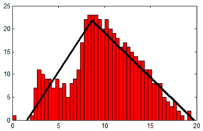
Figure 4: Comparison between the histogram of the eigenvalues of one random realization of the Laplacian matrix of a small-world model with parameters $N=512,$ $p=4/N$ and $k=3$, and the triangular function that fits the expected spectral moments.

We observe that the above estimation is valid for a large range in the values of the parameters. For example, in Fig. 5, we compare the values of the triangular abscissae $x_{1}$ and $x_{3}$ with the extreme points of the Laplacian spectral support, $\lambda_{2}$ and $\lambda_{n}$, for a small-world network with $N=512$ nodes, $k=3$, and $p$ in the range of values $\left[1/N:0.01/N:10/N\right].$ It is important to point out that, in this case too, the numerical values for the eigenvalues are obtained for one realization only, with no benefit from averaging. In the next section, we propose a methodology which uses results presented in previous sections to predict the local stability of the synchronous state in a small-world network of oscillators.

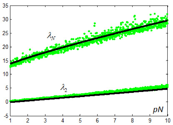
Figure 5: Comparison between the values of the triangular abscissae $x_{1}$ and $x_{3}$ with the extreme points of the Laplacian spectral support, $\lambda_{2}$ and $\lambda_{n}$, for a small-world network with $N=512$ nodes, $k=3$, and $p$ in the range of values $\left[1/N:0.01/N:10/N\right].$

IV Analytical Estimation of Synchronization

In this section we use the expressions in (17) and the triangular reconstruction in the above subsection to predict synchronization in a large small-world network of coupled nonlinear oscillators. Specifically, we study a network of coupled Rössler oscillators, as those in Example 1. We build our prediction based on the following steps:

1. Determine the region of synchronization following the technique presented in Subsection II-B. As illustrated in Example 1, the set of scaled eigenvalues $\{\gamma\lambda_{i}^{\left(K\right)}\}_{i=2,...,N}$ must lie in a certain region of stability, $S$, to achieve synchronization (in our example $S=\left(0,\sigma^{\ast}\approx 4.7\right)$).

2. Compute the expected spectral moments of the Laplacian eigenvalue spectrum for a given set of parameters using the set of Eqns. in (17).

3. Estimate the support of the Laplacian eigenvalue spectrum, $\{\lambda_{i}^{\left(K\right)}\}_{i=2,...,N}$, using the methodology presented in Subsection III-D. From Example 4, we have that $s_{l}=1.57$ and $s_{u}=19.76$ are good estimates of the lower and upper extremes of the spectral support, respectively.

4. Compare the region of stability in Step 1 with the estimation of the spectral support in Step 3, i.e., $\left(1.57~{}\gamma,19.76~{}\gamma\right)$.

Following the above steps, one can easily verify that our estimated spectral support, $\left(1.57~{}\gamma,19.76~{}\gamma\right)$, lies inside the region of stability, $\left(0,\sigma^{\ast}\approx 4.7\right)$, for $0<\gamma<4.7/19.76\approx 0.238$. Therefore, the small-world network of $512$ coupled Rössler oscillators is predicted to synchronize whenever the global coupling strength satisfies $\gamma\in\left(0,0.238\right)$.

IV-A Numerical Results

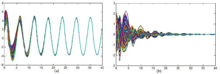
Figure 6: We plot the dynamics of the $x$-states for 512 Rössler oscillators (as the one described in Example 1) interconnected through the Small–World network with $p=4/N$ and $k=3$, in Fig.a. In Fig.b, we observe a clear exponential convergence of the errors towards zero.

In this section we present numerical simulations supporting our conclusions. We consider a set of identical $512$ Rössler oscillators (as the one described in Example 1) interconnected through the Small–World network defined in Example ($p=4/N$ and $k=3$). Using the methodology proposed above, we have predicted that the synchronous state of this system is locally stable if the coupling parameter $\gamma$ lies in the interval $\left(0,0.238\right)$. We run several simulations with the dynamics of the oscillators presenting different values of the global coupling strength $\gamma$. For each coupling strength, we present two plots: (i) the evolution of the $512$ $x$-states of the Rössler oscillators in the time interval $0\leq t\leq 40$, and (ii) the evolution of $x_{i}\left(t\right)-\bar{x}\left(t\right)$ for all $i$, where $\bar{x}\left(t\right)=\frac{1}{N}\sum_{i}x_{i}\left(t\right)$. Since our stability results are local, we have to carefully choose the initial states for the network of oscillators. For our particular choice of parameters, the (isolated) Rössler oscillator presents a stable limit cycle. For our simulations, we have chosen as initial condition for each oscillator in the network a randomly perturbed version of a particular point of this stable limit cycle. This particular point is $\mathbf{s}_{0}=\left(3.5119,-3.5332,0.2006\right)$. We have chosen the perturbed initial state for the $i$-th oscillator to be $\mathbf{s}_{0}+\mathbf{e}_{i}$, where $\mathbf{e}_{i}$ is a uniformly distributed random variable in the $3$-dimensional cube $\left[-2,2\right]^{3}$, and $\mathbf{e}_{i}$ is independent of $\mathbf{e}_{j}$ for $i\neq j$.I

In our first simulation, we use a coupling strength $\gamma=0.1\in\left(0,0.238\right)$; thus, we predict the synchronous state to be locally stable. Fig. 6 (a) and (b) represents the dynamics $x$-states for the 512 oscillators in the small-world network. In this case, we observe a clear exponential convergence of the errors to zero. In the second simulation, we choose $\gamma=0.3\notin\left(0,0.238\right)$; thus, we predict the synchronous state to be unstable. In fact, we observe in Figs. 7.a and 7.b how synchronization is clearly not achieved.

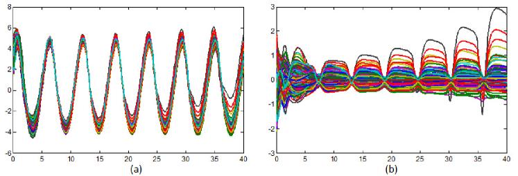
Figure 7: We plot the dynamics of the $x$-states for the 512 Rössler oscillators for $\gamma=0.3\notin\left(0,0.238\right)$ in Fig.a. We observe in Fig.b. how the errors do not converge to zero.

V Conclusions and Future Research

In this paper, we have studied the eigenvalue distribution of the Laplacian matrix of a large-scale small-world networks. We have focused our attention on the low-order moments of the spectral distribution. We have derived explicit expressions of these moments as functions of the parameters in the small-world model. We have then applied our results to the problem of synchronization of a network of nonlinear oscillators. Using our expressions, we have studied the local stability of the synchronous state in a large-scale small-world network of oscillators. Our approach is based on performing a triangular reconstruction matching the first three moments of the unknown spectral measure. Our numerical results match our predictions with high accuracy. Several questions remain open. The most obvious extension would be to derive expressions for higher-order moments of the Kirchhoff spectrum. A more detailed reconstruction of the spectral measure can be done based on more moments.

VI ACKNOWLEDGMENTS

The first author gratefully acknowledges George C. Verghese and Vincent Blondel for their comments and suggestions on this work.

References

- [1] A. L. Barabási, and R. Albert, “Emergence of Scaling in Random Networks,” Science, vol. 285, pp. 509-512, 1999.
- [2] M. di Bernardo, F. Garofalo, and F. Sorrentino, “Effects of Degree Correlation on the Synchronization of Networks of Oscillators,” International Journal of Bifurcation and Chaos, vol. 17, pp. 3499-3506, 2007.
- [3] N. Biggs, Algebraic Graph Theory, Cambridge University Press, second edition, 1993.
- [4] S. Boccaletti S., V. Latora, Y. Moreno, M. Chavez, and D.-H. Hwang, “Complex Networks: Structure and Dynamics,” Physics Reports, vol. 424, no. 4-5, pp. 175-308, 2006.
- [5] S. Boyd, A. Ghosh, B. Prabhakar and D. Shah, “Randomized Gossip Algorithms,” IEEE Trans. Inf. Theory, vol. 52, pp. 2508-2530, 2006.
- [6] P. Bremaud, Markov Chains: Gibbs Fields, Monte Carlo Simulation, and Queues, Springer, 2001.
- [7] F.R.K. Chung, Spectral Graph Theory, AMS: CBMS series, vol. 92, 1997.
- [8] S.N. Dorogovtsev, and J.F.F. Mendes, Evolution of Networks: From Biological Nets to the Internet and WWW, Oxford University Press, 2003.
- [9] M.O. Jackson, Social and Economic Networks, Princeton University Press, 2008.
- [10] A. Jadbabaie, J. Lin, and A. Morse, “Coordination of Groups of Mobile Autonomous Agents Using Nearest Neighbor,” IEEE Trans. Autom. Control, vol. 50, no.1, 2003.
- [11] X. Li, and G. Chen, “A Time-Varying Complex Dynamical Network Model and Its Controlled Synchronization Criteria,” IEEE Trans. Autom. Control, vol. 50, no.1, 2005.
- [12] L. Lovász, “Random Walks on Graphs: A Survey,” Combinatorics, Paul Erdös is Eighty (vol. 2), pp. 1-46, 2003.
- [13] J. Lu, X. Yu, G. Chen and D. Cheng, “Characterizing the Synchronizability of Small-World Dynamical Networks,” IEEE Trans. Circuits Syst. I, vol. 51, pp. 787-796, 2004.
- [14] S.C. Manrubia, A.S. Mikhailov, and D. Zanette, Emergence of Dynamical Order, World Scientific, 2004.
- [15] M.E.J. Newman, “The Structure and Function of Complex Networks,” SIAM Review vol. 45, pp. 167-256, 2003.
- [16] R. Olfati-Saber, J.A. Fax, and R.M. Murray, “Consensus and Cooperation in Networked Multi-Agent Systems,” Proc. IEEE, vol. 95, pp. 215-233, 2007.
- [17] L.M. Pecora, and T.L. Carroll, “Master Stability Functions for Synchronized Coupled Systems,” Phys. Rev. Lett., vol. 80, no. 10, pp. 2109-2112, 1998.
- [18] V.M. Preciado, Spectral Analysis for Stochastic Models of Large-Scale Complex Dynamical Networks, Ph.D. dissertation, Dept. Elect. Eng. Comput. Sci., MIT, Cambridge, MA, 2008.
- [19] J.-J.E. Slotine and W. Wang, “A Study of Synchronization and Group Cooperation using Partial Contraction Theory,” in Cooperative Control (S. Morse, N. Leonard, and V. Kumar, eds.), Lecture Notes in Control and Information Science, vol. 309, Springer-Verlag, 2004.
- [20] S.H. Strogatz, “Exploring Complex Networks,” Nature, vol. 410, pp. 268-276, 2001.
- [21] S.H. Strogatz, Sync: The Emerging Science of Spontaneous Order, New York: Hyperion, 2003.
- [22] D.J. Watts, and S. Strogatz, “Collective Dynamics of Small World Networks,” Nature, vol 393, pp. 440-42, 1998.
- [23] C.W. Wu, “Synchronization in Arrays of Coupled Nonlinear Systems: Passivity, Circle Criterion, and Observer Design,” IEEE Trans. Circuits Syst. I, vol. 48, pp. 1257-1261, 2001.