Spectral Analysis of Virus Spreading in Random Geometric Networks

Abstract

In this paper, we study the dynamics of a viral spreading process in random geometric graphs (RGG). The spreading of the viral process we consider in this paper is closely related with the eigenvalues of the adjacency matrix of the graph. We deduce new explicit expressions for all the moments of the eigenvalue distribution of the adjacency matrix as a function of the spatial density of nodes and the radius of connection. We apply these expressions to study the behavior of the viral infection in an RGG. Based on our results, we deduce an analytical condition that can be used to design RGG’s in order to tame an initial viral infection. Numerical simulations are in accordance with our analytical predictions.

I Introduction

The analysis of spreading processes in large-scale complex networks is a fundamental dynamical problem in network science. The relationship between the dynamics of epidemic/information spreading and the structure of the underlying network is crucial in many practical cases, such as the spreading of worms in a computer network, viruses in a human population, or rumors in a social network. Several papers approached different facets of the virus spreading problem. A rigorous analysis of epidemic spreading in a finite one-dimensional linear network was developed by Durrett and Liu in [3]. In [10], Wang et al. derived a sufficient condition to tame an epidemic outbreak in terms of the spectral radius of the adjacency matrix of the underlying graph. Similar results were derived by Ganesh et al. in [4], establishing a connection between the behavior of a viral infection and the eigenvalues of the adjacency matrix of the network.

In this paper, we study the dynamics of a viral spreading in an important type of proximity networks called Random Geometric Graphs (RGG). RGG’s consist of a set of vertices randomly distributed in a given spatial region with edges connecting pairs of nodes that are within a given distance $r$ from each other (also called connectivity radius). In this paper, we derive new explicit expressions for the expected spectral moments of the random adjacency matrix associated to an RGG. Our results allow us to derive analytical conditions under which an RGG is well-suited to tame an infection in the network.

The paper is structured as follows. In Section II, we describe random geometric graphs and introduce several useful results concerning their structural properties. We also present the spreading model in [10] and review an important result that relates the behavior of an initial infection with the spectral radius of the adjacency matrix. In Section III, we study the eigenvalue spectrum of random geometric graphs. We derive explicit expressions for the expected spectral moments in the case of one- and two-dimensional RGG’s. In Section IV, we use these expressions to study the spectral radius of RGG’s. Our results allow us to design RGG’s with the objective of taming epidemic outbreaks. Numerical simulations in Section IV validate our results.

II Virus Spreading in Random Geometric Graphs

In this section, we briefly describe random geometric graphs and introduce several useful results concerning their structural properties (see [7] for a thorough treatment). We then describe the spreading model introduced in [10] and show how to study the behavior of an infection in the network from the point of view of the adjacency eigenvalues.

II-A Random Geometric Graphs

Consider a set of $n$ nodes, $V_{n}=\{v_{1},...,v_{n}\}$, respectively located at random positions, $\chi_{n}=\{\mathbf{x}_{1},...,\mathbf{x}_{n}\}$, where $\mathbf{x}_{i}$ are i.i.d. random vectors uniformly distributed on the $d$-dimensional unit torus, $\mathbb{T}^{d}$. We use the torus for convenience, to avoid boundary effects. We then connect two nodes $v_{i},v_{j}\in V_{n}$ if and only if $\left\|\mathbf{x}_{i}-\mathbf{x}_{j}\right\|\leq r$, where $r$ is the so-called connectivity radius. In other words, a link exists between $v_{i}$ and $v_{j}$ if and only if $v_{j}$ lies inside the sphere of radius $r\left(n\right)$ centered at $v_{i}$. We denote this spherical region by $S_{i}\left(r\right)$, and the resulting random geometric graph by $G\left(\chi_{n};r\right)$. We define a walk of length $k$ from $v_{0}$ to $v_{k}$ as an ordered set of (possibly repeated) vertices $\left(v_{0},v_{1},...,v_{k}\right)$ such that $v_{i}\sim v_{i+1},$ for $i=0,1,...,k-1$; if $\nu_{k}=\nu_{0}$ the walk is said to be closed.

The degree $d_{i}$ of a node $v_{i}$ is the number of edges connected to it. In our case, the degrees are identical random variables with expectation [7]:

$$\mathbb{E}\left[d_{i}\right]=nV^{\left(d\right)}r^{d},$$ (1)

where $V^{\left(d\right)}$ is the volume of a $d$-dimensional unit sphere, $V^{\left(d\right)}=\pi^{d/2}\left/\Gamma\left(d/2+1\right)\right.$, and $\Gamma\left(\cdot\right)$ is the Gamma function. The clustering coefficient is a measure of the number of triangles in a given graph, where a triangle is defined by the set of edges $\left\{\left(i,j\right),\left(j,k\right),\left(k,i\right)\right\}$ such that $i\sim j\sim k\sim i$. For one- and two-dimensional RGG’s we can derive an explicit expression for the expected number of triangles, $\mathbb{E}\left[t_{i}\right]$, touching a particular node $v_{i}$ (details are provided in Section III).

The adjacency matrix of an undirected graph $G,$ denoted by $A(G)=[a_{ij}]$, is defined entry-wise by $a_{ij}=1$ if nodes $i$ and $j$ are connected, and $a_{ij}=0$ otherwise. (Note that $a_{ii}=0$ for simple graphs.) Denote the eigenvalues of a $n\times n$ symmetric adjacency matrix $A(G)$ by $\lambda_{1}\leq...\leq\lambda_{n}$. The $k$-th order moment of the eigenvalue spectrum of $A(G)$ is defined as:

$$m_{k}(G)=\frac{1}{N}\sum_{i=1}^{n}\lambda_{i}^{k}$$

(which is also called the $k$-th order spectral moment).

We are interested in studying asymptotic properties of the sequence $G(\chi_{n};r\left(n\right))$ for some sequence $\left\{r\left(n\right):n\in\mathbb{N}\right\}$. In [7], two particularly interesting regimes are introduced: the thermodynamic limit with $nr\left(n\right)^{d}\rightarrow\alpha\in\left(0,\infty\right)$, so that the expected degree of a vertex tends to a constant, and the connectivity regime with $r\left(n\right)\rightarrow\gamma\left(\frac{\log n}{n}\right)^{1/d}$ with a constant $\gamma$, so that the expected degree of the nodes grows as $c\log n$. In this paper, we focus on studying the spectral moments in the connectivity regime. In Section III, we derive explicit expressions for the expected spectral moments of $G\left(\chi_{n};r_{n}\right)$ for any network size $n$. We then use this information to bound the spectral radius of the adjacency matrix of $G(\chi_{n};r\left(n\right))$.

II-B Spectral Analysis of Virus Spreading

In this section, we briefly review an automaton model that describes the dynamics of a viral infection in a specific network of interactions. This model was proposed and analyzed in [10], where a connection between the growth of an initial infection in the network and the spectral radius of the adjacency matrix was established. This model involves several parameters. First, the infection rate $\beta$ represents the probability of a virus at an infected node $i$ spreading to another neighboring node $j$ during a time step. Also, we denote by $\delta$ the probability of recovery of any infected node at each time step. For simplicity, we consider $\beta$ and $\delta$ to be constants for all the nodes in $G$. We also denote by $p_{i}\left[k\right]$ the probability that node $i$ is infected at time $k$. The evolution of the probability of infection is modeled by means of the following system of non-linear difference equation:

$$p_{i}\left[k+1\right]=[1-\prod_{j\in\mathcal{N}_{i}}\left(1-\beta\,p_{j}\left[k\right]\right)]+\left(1-\delta\right)p_{i}\left[k\right],$$ (2)

for $i=1,...,n$, where $\mathcal{N}_{i}$ denotes the set of nodes connected to node $i$. We are interested in studying the dynamics of the system for a low-density level of infection, i.e., $\beta\,p_{j}\left[k\right]\ll 1$. In this regime, a sufficient condition for a small initial infection to die out is [10]:

$$\lambda_{\max}\left(A(G)\right)<\frac{\delta}{\beta}.$$ (3)

One can prove that (3) is a sufficient condition for local stability around the disease-free state. Thus, we can use condition (3) to design networks with the objective of taming initial low-density infections.

III Spectral Analysis of Random Geometric Graphs

In this paper, we study the eigenvalue distribution of the random adjacency matrix associated to $G(\chi_{n};r\left(n\right))$ for $n\rightarrow\infty$. In this section, we characterize eigenvalue distribution using its sequence of spectral moments. In our derivations, we use an interesting graph-theoretical interpretation of the spectral moments [1]: the $k$-th spectral moment of $G$ is proportional to the number of closed walks of length $k$ in $G$. This result allows us to transform the algebraic problem of computing spectral moments of the adjacency matrix into the combinatorial problem of counting closed walks in the graph. In the following subsection, we compute the expected value of the number of closed walks of length $k$ in $G(\chi_{n};r\left(n\right))$.

III-A Spectral Moments of One-Dimensional RGG’s

As we mentioned above, we can compute the $k$-th spectral moment of a graph by counting the number of closed walks of length $k$. In the case of an RGG $G(\chi_{n};r\left(n\right))$, this number is a random variable. In this subsection, we introduce a novel technique to compute the expected number of closed walks of length $k$. For clarity, we introduce our technique for the first three expected spectral moments $k=1,2,3$. We then use these results to induce a general expression for higher-order moments in one-dimensional RGG’s.

The first-order spectral moment is equal to the number of closed walks of length $k=1$. Since $G(\chi_{n};r)$ is a simple graphs with no self-loops, we have that $m_{1}\left(G(\chi_{n};r)\right)$ is a deterministic quantity equal to $0$.

We now study the expected second moment, $\mathbb{E}\left[m_{2}\left(G(\chi_{n};r)\right)\right]$, by counting the number of closed walks of length two. In simple graphs, the only possible closed walks of length two are those that start at a given node $v_{i}$, visit a neighboring node $v_{j}\in\mathcal{N}_{i}$, and return back to $v_{i}$. Hence, the number of closed walks of length two starting at $v_{i}$ is equal to $d_{i}$. Thus, from (1), we have

$$\mathbb{E}\left[m_{2}\right]=\frac{1}{n}\sum_{i=1}^{n}\mathbb{E}\left[d_{i}\right]=nV^{\left(d\right)}r^{d}\text{,}$$

where this result is valid for any dimension $d\geq 1$.

The third spectral moment is proportional to the number of closed walks of length three in the graph. We now derive an expression for the expected number of triangular walks starting at a given node $v_{i}$ in a one-dimensional RGG. Since all nodes are statistically equivalent, our result is valid for any other starting node. For simplicity in our calculations, we consider that $v_{i}$ is located at the origin. A triangular walk starting at node $v_{i}$ exists if and only if there exist two nodes $v_{j}$ anv $v_{k}$ such that $\left|x_{j}\right|\leq r$, $\left|x_{k}\right|\leq r$, and $\left|x_{k}-x_{j}\right|\leq r$. Also, since the random distribution of vertices on $\mathbb{T}^{1}$ is uniform (with density $n$), the probability of nodes $v_{j}$ and $v_{k}$ being respectively located in the differential lengths $\left[x_{j}+dx_{j}\right)$ and $\left[x_{k}+dx_{k}\right)$ is equal to $n^{2}~{}dx_{j}dx_{k}$. Hence, one can compute the expected number of triangular walks starting at node $v_{i}$ as

$$\mathbb{E}\left[t_{i}\right]=\int\int_{\left(x_{j},x_{k}\right)\in H_{2}\left(r\left(n\right)\right)}n^{2}~{}dx_{j}dx_{k},$$

where

$$H_{2}\left(r\right) =\left\{\left(x_{j},x_{k}\right)\in\mathbb{T}^{2}\text{ s.t. }\left|x_{j}\right|\leq r,\right.$$ (4)

$$\left.\text{ \ \ \ \ \ }\left|x_{k}-x_{j}\right|\leq r,\left|x_{k}\right|\leq r\right\}.$$

Thus, $\mathbb{E}\left[t_{i}\right]$ can be computed as $n^{2}$Vol$\left[H_{2}\left(r\left(n\right)\right)\right]$ (where Vol$\left(H\right)$ denotes the volume contained by the polyhedron $H$.) Notice that $H_{2}\left(r\right)$ can be defined by a set of linear inequalies; hence, $H_{2}\left(r\right)$ is a convex polyhedron that depends on $r$. Furthermore, the set of linear inequalities in (4) presents a homogeneous dependency with respect to the parameter $r$. Therefore, we can write Vol$(H_{2}\left(r\right))$ as $r^{2}$Vol$(H_{2}\left(1\right))$. Finally, one can easily compute the volume of $H_{2}\left(1\right)$ to be equal to $3$. Thus, the expected third spectral moment of a one-dimensional RGG is given by

$$\mathbb{E}\left[m_{3}\right]=\frac{1}{n}\sum_{i=1}^{n}\mathbb{E}\left[t_{i}\right]=3n^{2}r^{2}.$$

In the following, we extend the above technique to compute higher-order expected spectral moments. Denote by $W_{i}^{\left(k\right)}$ the number of closed walks of length $k$ starting at node $v_{i}$ in $G(\chi_{n};r\left(n\right))$. Regarding $W_{i}^{\left(k\right)}$, we derive the following result.

Theorem 1

The expected number of closed walks of length $k$, $W_{i}^{\left(k\right)}$, in a random geometric graph, $G(\chi_{n};r)$, on $\mathbb{T}^{1}$ is given by

$$\mathbb{E}\left[W_{i}^{\left(k\right)}\right]=\left(nr\right)^{k-1}\frac{1}{2\left(k-1\right)!}\sum_{j=1}^{k-2}\binom{k-1}{j-1}~{}E_{k-1,j},$$

where $E_{k-1,j}$ are the Eulerian numbers .

Proof:

Consider a particular closed walk, $\mathbf{w}_{k}=\left(v_{1},v_{2},v_{3},...,v_{k},v_{1}\right)$, of length $k$ starting and ending at node $v_{1}$ (which we locate at zero for computational convenience). A walk $\mathbf{w}_{k}$ exists if and only if there exists a set of $k-1$ nodes, $\left\{v_{2},v_{3},...,v_{k}\right\},$ such that $\left|x_{1}\right|\leq r$, $\left|x_{j+1}-x_{j}\right|\leq r$ for $j=2,...,k-1$, and $\left|x_{k}\right|\leq r$. Since the distribution of vertices on $\mathbb{T}^{1}$ is uniform (with density $n$) one can compute the expectation of $W_{i}^{\left(k\right)}$ as

$$\mathbb{E}\left[W_{i}^{\left(k\right)}\right]=\int_{(x_{2},...,x_{k})\in H_{k-1}\left(r\left(n\right)\right)}n^{k-1}~{}dx_{2}...dx_{k},$$

where

$$H_{k-1}\left(r\right) =\left\{(v_{2},v_{3},...,v_{k})\in\mathbb{T}^{k-1}\text{ s.t. }\left|v_{2}\right|\leq r,\right.$$ (5)

$$\left.\text{ \ \ }\left|x_{j+1}-x_{j}\right|\leq r\text{ for }j=2,...,k-1,\right.$$

$$\left.\text{ \ \ \ }\left|x_{k}\right|\leq r\right\}.$$

Thus, $\mathbb{E[}W_{i}^{\left(k\right)}]$ can be computed as $n^{k-1}$Vol$\left[H_{k-1}\left(r\right)\right]$, where $H_{k-1}\left(r\right)$ is a convex polyhedron defined by a set of linear inequalities. Finally, note that the homogeneous structure of the system of linear inequalities defining $H_{k-1}\left(r\right)$ allows us to write Vol$(H_{k-1}\left(r\right))=r^{k-1}$Vol$(H_{k-1}\left(1\right))$. Therefore,

$$\mathbb{E}\left[W_{i}^{\left(k\right)}\right]=\left(nr\right)^{k-1}\text{Vol}\left(H_{k-1}\left(1\right)\right).$$ (6)

The volume of $H_{k-1}\left(1\right)$ is a particular number, independent of the RGG parameters, i.e., $n$ and $r$. Furthermore, we have found an explicit analytical expression for the volume of $H_{k}\left(1\right)$ for any $k\geq 1$. Although we do not provide details of our derivation, due to space limitations, an explicit expression for the volume of $H_{k}\left(1\right)$ is given by [9]:

$$\text{Vol}\left(H_{k}\left(1\right)\right)=\frac{2}{k!}\sum_{j=1}^{k-1}\binom{k}{j-1}~{}E_{k,j},$$ (7)

where $E_{d,k}$ denotes the Eulerian numbers. Substituting (7) in (6) we obtain the statement of our lemma. ∎

In [6], Lasserre proposed an algorithm to compute the volume of a polyhedron defined by a set of linear inequalities. We can use this algorithm to verify the validity of (5). Applying this algorithm to the set of inequalities in (5), we compute the following volumes for $k=1,...,10$:

$$H_{1} =2,~{}H_{2}=3,~{}H_{3}=5.333...,~{}H_{4}=9.58333...,$$

$$H_{5} =17.6000...,~{}H_{6}=32.70555...,~{}H_{7}=61.3587...,$$

$$H_{8} =115.947...,~{}H_{9}=220.3238...,~{}H_{10}=420.825...$$

These numerical values match perfectly with our analytical expression in Theorem 1.

If $nr\left(n\right)=\Omega\left(\log n\right)$ (i.e., the average degree grows as $\log n$, or faster), one can prove that $\mathbb{E}\left[m_{k}\right]=\left(1+O\left(\log^{-1}n\right)\right)~{}\mathbb{E[}W_{i}^{\left(k\right)}]$. Hence, from (6) and (7), we have the following closed-form expression for the asymptotic expected spectral moments:

$$\mathbb{E}\left[m_{k}\right]\asymp\left(nr\right)^{k-1}\frac{1}{2\left(k-1\right)!}\sum_{j=1}^{k-2}\binom{k-1}{j-1}~{}E_{k-1,j}.$$ (8)

In the following table we compare the analytical result in (8) with numerical realizations of the empirical spectral moments. In our simulations, we distribute $n=1000$ nodes uniformly in $\mathbb{T}^{1}$ and choose a connectivity radius $r=0.01$ (which results in an average degree $\mathbb{E}[d_{i}]=20$). The second, third, and forth column in the following table represent the analytical expectations of the spectral moments, the empirical average of the spectral moments from 10 random realizations of the RGG, and the corresponding empirical typical deviation, respectively.

$$k$$ Empirical Average Typical Deviation

1 0 1.38e-16 1.3e-15

2 20 19.9326 0.0976

3 300 297.284 4.3598

4 5,733 5,956.30 196.94

Our numerical results present an excellent match with our analytical predictions.

III-B Spectral Moments of Two-Dimensional RGG’s

In this subsection, we derive expressions for the first three expected spectral moments of $G(\chi_{n};r\left(n\right))$ when the nodes are uniformly distributed in $\mathbb{T}^{2}$. The expressions for the first and second expected spectral moments are $m_{1}=0$ and $\mathbb{E}\left[m_{2}\right]=\pi nr^{2}$. The third spectral moment is proportional to the number of closed walks of length three in the graph. In the two-dimensional case, we count the number of triangular walks using a technique that we illustrate in Fig. 1. In this figure, we plot two nodes $v_{i}$ and $v_{j}$. The parameters $\rho$ and $\phi$ in Fig. 1 denote the distance and angle between these two nodes, i.e., $\rho\triangleq\left\|\mathbf{x}_{j}-\mathbf{x}_{i}\right\|$ and $\phi=\measuredangle\left(\mathbf{x}_{j}-\mathbf{x}_{i}\right)$. An edge between $v_{i}$ and $v_{j}$ exists if an only if $v_{j}$ is located inside the circle $S_{i}\left(r\right)$. In this setting, the probability of existence of a triangle touching both $v_{i}$ and $v_{j}$ is equal to the probability of a third node $v_{k}$ being in the shaded area $A_{l}$ (see Fig. 1). This area is the result of intersecting the circles $S_{i}\left(r\right)$ and $S_{j}\left(r\right)$, and the resulting probability is equal to $n~{}A_{l}$. The intersecting region $A_{l}$ is a symmetric lens which area can be computed as a function of $\rho$ and $r$ as follows:

$$A_{l}\left(\rho;r\right)=\left\{\begin{array}[]{cc}2r^{2}\cos^{-1}\left(\frac{\rho}{2r}\right)-\frac{\rho}{2}\sqrt{4r^{2}-\rho^{2}},&\text{for }\rho\leq r,\\ 0,&\text{for }\rho>r.\end{array}\right.$$ (9)

Therefore, we can compute the expected number of triangles by integrating over the set of all possible positions of $v_{j}$, i.e., $\eta\in\left[0,r\right]$ and $\phi\in[0,2\pi)$, as follows

$$\mathbb{E}\left[t_{i}\right]=\int_{\rho=0}^{r}\int_{\phi=0}^{2\pi}n^{2}A_{l}\left(\rho;r\right)~{}\rho~{}d\rho~{}d\phi.$$ (10)

After substituting (9) in (10), we can explicitly solve the resulting integral to be

$$\mathbb{E}\left[t_{i}\right]=\left(\pi-\frac{3\sqrt{3}}{4}\right)\pi\left(nr^{2}\right)^{2}\approx 5.78\left(nr^{2}\right)^{2}.$$ (11)

Consequently, we have the following expression for the third expected spectral moment $\mathbb{E}\left[m_{3}\right]=\frac{1}{n}\sum_{i=1}^{n}\mathbb{E}\left[t_{i}\right]=\mathbb{E}\left[t_{i}\right]$.

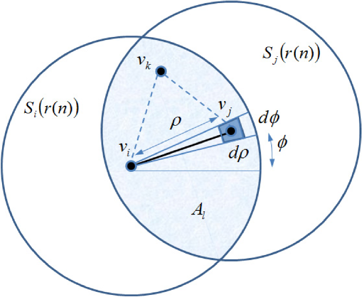
Figure 1: This figure illustrates the technique proposed in Section III.B to count the number of triangular walks in a two-dimensional RGG.

In the following, we extend the technique introduced above to compute closed walks of arbitrary length. Denote by $W_{i}^{\left(k\right)}$ the number of closed walks of length $k$ starting at node $v_{1}$ in $G(\chi_{n};r\left(n\right))$. The idea behind our technique is illustrated in Fig. 2, where we represent a particular closed walk of length $6$. We denote this walk by $\mathbf{w}_{k}=\left(v_{1},v_{2},...,v_{k-1},v_{k},v_{1}\right)$. We define the following set of relative distances and angles between every pair of connected vertices: $\rho_{i}\triangleq\left\|\mathbf{x}_{i+1}-\mathbf{x}_{i}\right\|$ and $\phi_{i}=\measuredangle\left(\mathbf{x}_{i+1}-\mathbf{x}_{i}\right)$ for $i=1,...,k-2$. We also define the following parameter

$$\rho=\left|\sum_{j=1}^{k-2}\rho_{j}e^{\mathbf{i}\alpha_{j}}\right|,$$ (12)

($\mathbf{i}=\sqrt{-1}$) which is the resulting distance between nodes $v_{k-1}$ and $v_{1}$ given a particular set of distances and angles $\left\{\left(r_{i},\phi_{i}\right)\right\}_{i=1,...,k-2}$ (see Fig. 2). In this setting, the conditional probability of existence of a walk $\mathbf{w}_{k}=\left(v_{1},v_{2},...,v_{k-1},v_{k},v_{1}\right)$ given the set of relative positions, $\left\{\left(r_{i},\phi_{i}\right)\right\}_{i=1,...,k-2}$, is equal to the probability of $v_{k}$ being in the shaded area $A_{l}$ in Fig. 2. We have an expression for this area in (9), where $\rho$ is defined in (12). Finally, we can compute the expectation of $W_{i}^{\left(k\right)}$ by performing an integration over the set of all possible positions (i.e., $\rho_{j}\in\left[0,r\right]$ and $\phi_{j}\in[0,2\pi)$ for $j=2,...,k-1$), as follows

$$\mathbb{E}\left[W_{i}^{\left(k\right)}\right]=n^{k-1}\int_{\left(\mathbf{\eta,\varphi}\right)\in C_{k-2}}A_{l}\left(\rho;r\right)~{}\prod_{j=2}^{k-1}\eta_{j}~{}d\mathbf{\eta~{}}d\mathbf{\varphi,}$$

where $\mathbf{\eta=}\left(\rho_{2},...,\rho_{k-1}\right)$, $\mathbf{\varphi}=\left(\phi_{2},...,\phi_{k-1}\right)$, and $C_{k-2}=\{\left(\mathbf{\eta,\varphi}\right):\mathbf{\eta\in}\left[0,r\right]^{k-2}$ and $\mathbf{\varphi}\in[0,2\pi)^{k-2}\}$. Although a closed-form for the above expression can only be computed for $k\leq 3$, we can always find a good approximation via numerical integration. For example, the integration for $k=4$ gives us $\mathbb{E[}W_{i}^{\left(4\right)}]\approx 14.2511\left(nr^{2}\right)^{3}$.

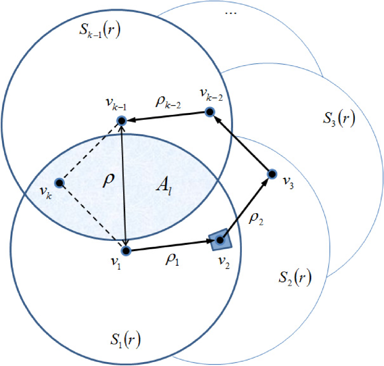
Figure 2: This figure illustrates the technique proposed in Section III.B to count the number of closed walks of length $k$ in a two-dimensional RGG.

In the following table, we compare our analytical results with numerical realizations of the empirical spectral moments of a two-dimensional RGG. In our simulations, we distribute $n=1000$ nodes uniformly on $\mathbb{T}^{2}$ and choose a connectivity radius $r=\sqrt{50/\pi n}\approx 0.1784$ (which results in an average degree $\mathbb{E}[d_{i}]=50$). The second, third, and forth columns in the following table represent the analytical expectation of the spectral moments, the empirical average from 10 random realizations, and the corresponding empirical typical deviation, respectively.

$$k$$ Empirical Average Typical Deviation

1 0 -9.2e-16 1.1e-15

2 50 50.0820 0.3908

3 1,464.1 1,475.8 37.3777

4 59,452 60,127 2,955.3

Our numerical results present an excellent match with our analytical predictions.

In the following section, we use the results introduced in this section to study the spreading of an infection in a random geometric network.

IV Spectral Analysis of Virus Spreading

In this section, we use the expressions for the expected spectral moments to design random geometric networks to tame an initial viral infection in the network. In our design problem, we consider that the size of the network $n$ and the parameters in (2), i.e., $\beta$ and $\delta$, are given. Hence, our design problem is reduced to studying the range of values of $r$ for which the RGG is well-suited to tame an initial viral infection.

A sufficient condition for local stability around the disease-free state was given in (3). Thus, we have to find the range of values of $r$ for which the associated spectral radius $\lambda_{\max}$ is smaller than the ratio $\delta/\beta$. In the following subsection, we show how to derive an analytical upper bound for the spectral radius based on the expected spectral moments.

IV-A Analytical Upper Bound for the Spectral Radius

In order to upper-bound the spectral radius, we use Wigner’s high-order moment method [11]. This method provides a probabilistic upper bound based on the asymptotic behavior of the $k$-th expected spectral moments for large $k$. We present the details for a one-dimensional RGG, although the same technique can be applied to RGG’s in higher dimensions. For a one-dimensional RGG in the connectivity regime, we derived an explicit expression for the expected spectral moments in (8). A logarithmic plot of Vol$\left(H_{k}\left(1\right)\right)$ for $k=1,2,...,9$ unveils that Vol$\left(H_{k}\left(1\right)\right)\rightarrow\beta_{1}c_{1}^{k}$ for large-order moments (a line in logarithmic scale), where, from a numerical fitting, we find that $\beta_{1}=0.35$ and $c_{1}=1.9192$. Therefore, from (8) we have

$$\mathbb{E}\left[m_{k}\right]\asymp\beta_{1}\left(c_{1}nr\right)^{k},$$

for large $k$.

For even-order expected spectral moments (i.e., $k=2s$ for $s\in\mathbb{N}$), the following holds

$$\mathbb{E}\left[m_{2s}\right]=\frac{1}{n}\sum_{i=1}^{n}\mathbb{E}[\lambda_{i}^{2s}]\geq\frac{1}{n}\mathbb{E}[\lambda_{\max}^{2s}].$$

Define $f\left(n\right)=n^{1-\delta}\log n$; thus, for any $\varepsilon,\delta>0$ (and $c_{1}=1.9192$), we can apply Markov´s inequality as follows

$$\mathbb{P}\left(\lambda_{\max}^{2s}\geq(c_{1}nr+\varepsilon rf\left(n\right))^{2s}\right) \leq \frac{\mathbb{E}[\lambda_{\max}^{2s}]}{(c_{1}nr+\varepsilon rf\left(n\right))^{2s}}$$

$$\leq \frac{n~{}\mathbb{E}\left[m_{2s}\right]}{(c_{1}nr+\varepsilon rf\left(n\right))^{2s}},$$

For large $s$, one can prove that [8]

$$\mathbb{P}\left(\lambda_{\max}\geq c_{1}nr+\varepsilon rf\left(n\right)\right)\leq n\beta_{1}\exp\left(-\frac{\varepsilon}{c_{1}}sn^{-\delta}\log n\right).$$

Assuming that $s$ grows as $\beta_{2}n^{\delta}$, for $\beta_{2},\delta>0$, we have

$$\mathbb{P}\left(\lambda_{\max}\geq c_{1}nr+\varepsilon rf\left(n\right)\right)\leq n\beta_{1}\exp\left(-\frac{\beta_{2}\varepsilon}{c_{1}}\log n\right)=o\left(1\right),$$

for all sufficiently large $\varepsilon$. Thus,

$$\lim_{n\rightarrow\infty}\mathbb{P}\left(\lambda_{\max}<c_{1}nr+\varepsilon rn^{1-\delta}\log n\right)=1.$$ (13)

In other words, $\lambda_{\max}$ is upper-bounded by $cnr+\varepsilon rn^{1-\delta}\log n$ with probability $1$ for $n\rightarrow\infty$. In practice, for a large (but finite) $n$, we can use $1.9192~{}nr$ as an upper bound of $\lambda_{\max}$. In Fig. 4, we plot the empirical spectral radius of an RGG with $n=1000$ and $r\left(n\right)=\bar{d}/2n$, with expected degrees $\bar{d}=[$10:1:100$]$ (circles in the figure). We also plot the values of our analytical upper bound, $1.9192~{}nr$, in solid line.

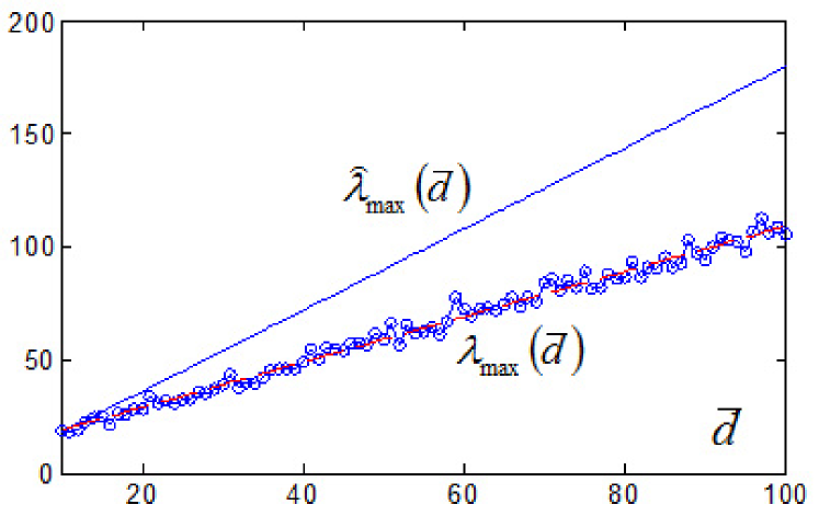
Figure 3: Comparison between the empirical spectral radius of an RGG (circles in the plot) and the values of our analytical upper bound (solid line) for $n=1000$ and $r\left(n\right)=\bar{d}/2n$, with expected degrees $\bar{d}=[$10:1:100$]$.

The technique introduced in this subsection is also valid for RGG’s in higher-dimensions. In general, one can prove that for a $d$-dimensional RGG that the expected spectral moment grows as $\mathbb{E}\left[m_{k}\right]\rightarrow\beta_{d}\left(c_{d}nr^{d}\right)^{k}$. Applying Wigner’s high-order moment method to this sequence, one can derive a probabilistic upper bound similar to (13). In particular, we have that $\lambda_{\max}<c_{d}nr^{d}$ for large $n$ with high probability. In the following subsection, we use our results to design the connectivity radius of an RGG in order to tame an initial viral infection.

IV-B Spectral Radius Design

Once the spectral radius is upper-bounded, our design problem becomes trivial. Since (3) represents a sufficient condition for local stability around the disease-free state, we have the following condition to tame an initial viral infection for a $d$-dimensional RGG:

$$\lambda_{\max}\left(G(\chi_{n};r\right))<c_{d}nr^{d}<\frac{\delta}{\beta},$$

which implies the following design condition for the connectivity radius:

$$r<\left(\frac{\delta}{\beta c_{d}n}\right)^{1/d},$$ (14)

where $c_{d}$ is a positive constant that depends on the dimension of $\mathbb{T}^{d}$. For example, in the one-dimensional case, we have $c_{1}=1.9192$; hence, (14) becomes $r<\delta/\left(1.9192~{}\beta n\right)$. We now validate this result with several numerical simulations of a viral infection in a one-dimensional RGG.

Consider an RGG with $n=1000$ nodes and a connectivity radius of $r=0.005$ (which implies an average degree of $10$). The resulting spectral radius in this RGG is $\lambda_{\max}=17.2629$. In our numerical simulations, we choose the initial probability of infection to be $p_{i}\left[0\right]\sim 0.01$Unif$[0,1]$; hence, approximately $1\%$ of the nodes in the network are initially infected. In our first experiment, we choose a rate of infection $\beta=0.020$, and a recovery rate $\delta=0.018$. Since the sufficient condition for viral control in (14) is not satisfied, we cannot guarantee an initial infection to be tamed. In Fig. 5 we show an image of the evolution of the probability of infection for this case. This figure is a color map for the simultaneos evolution of $p_{i}\left[n\right]$ for $i=1,...,1000$. Each horizontal line represents the value of $p_{i}\left[n\right]$ for a particular $i$. In this color map, blue represents a zero value, green and yellow tones represent intermediate values, and red represents values close to one. On the other hand, if we increase the recovery rate to $\delta=0.35$ keeping the rest of parameters fixed, we have that $\delta/\beta=17.50>\lambda_{\max}$ and we satisfy condition (3). Hence, the probability of infection of every node is guaranteed to converge towards zero. In Fig. 6, we observe the color map for the evolution of the probability of infection in this case, where we clearly observe how $p_{i}\left[n\right]\rightarrow 0$ for all $i$. Hence, this latter RGG is well-suited to tame initial viral infections.

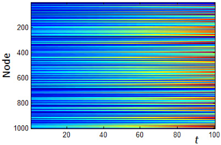
Figure 4: Color map representing the evolution of the probabilities of infection $p_{i}\left[n\right]$ for $i=1,...,1000$ in an RGG with $n=1000$ nodes, connectivity radius $r=0.005$, rate of infection $\beta=0.020$, and recovery rate $\delta=0.018$. Each horizontal line represents the value of $p_{i}\left[n\right]$ for a particular $i$. In this color map, blue represents a zero value, green and yellow tones represent intermediate values, and red represents values close to one. In this case, we observe an epidemic outbreak.

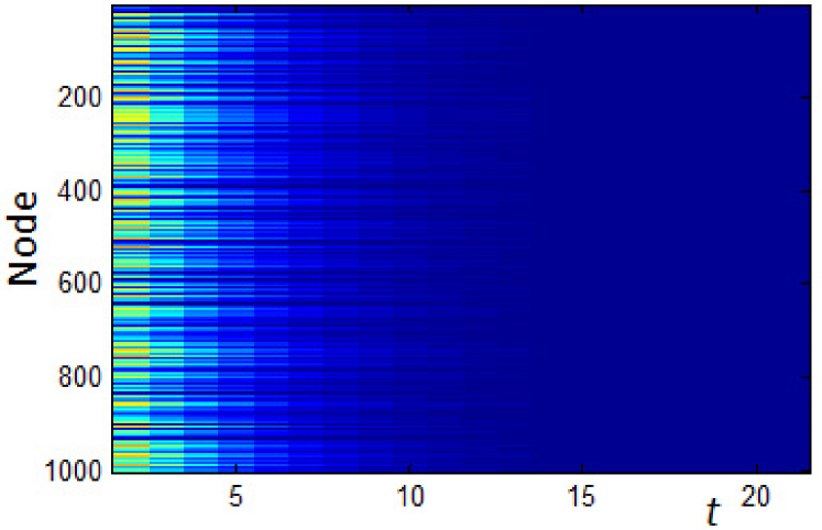
Figure 5: Color map representing the evolution of the probabilities of infection $p_{i}\left[n\right]$ when we increase the recovery rate to $\delta=0.35$ (the rest of parameters are the same as we used for Fig. 5). We observe how the probability of infection of every node converges towards zero in this case.

V Conclusions

In this paper, we have studied the spreading of a viral infection in a random geometric graph from a spectral point of view. We have focused our attention on studying the eigenvalue distribution of the adjacency matrix. We have derived, for the first time, explicit expressions for the spectral moments of the adjacency matrix as a function of the density of nodes and the connectivity radius. We have then applied our results to the problem of viral spreading in a network with a low-density infection. Using our expressions, we have derived upper bounds for the spectral radius of the adjacency matrix. Finally, we have applied this upper bound to design random geometric graphs that are well-suited to tame an initial low-density infection. Our numerical results match our predictions with high accuracy.

References

- [1] N. Biggs, Algebraic Graph Theory, 2nd Edition. Cambridge University Press, 1993.
- [2] P. Blackwell, M. Edmondson-Jones, and J. Jordan, “Spectra of Adjacency Matrices of Random Geometric Graphs,” Preprint.
- [3] R. Durrett and X.-E. Liu, “The Contact Process on a Finite Set,” Annals of Probability, vol. 16, pp. 1158-1173, 1988.
- [4] A. Ganesh, L. Massoulie, and D. Towsley, “The Effect of Network Topology on the Spread of Epidemics,” Proc. IEEE INFOCOM ’05, pp. 1455-1466, 2005.
- [5] R.L. Graham, D.E. Knuth, and O. Patashnik, Concrete Mathematics: A Foundation for Computer Science, Second Edition, Addison-Wesley, 1994.
- [6] J.B. Lasserre, “An Analytical Expression and an Algorithm for the Volume of a Convex Polyhedron in ,” J. Optim. Theor. Appl., vol. 39, pp. 363–377, 1983.
- [7] M. Penrose, Random Geometric Graphs, Oxford University Press, 2003.
- [8] V.M. Preciado, Spectral Analysis for Stochastic Models of Large-Scale Complex Dynamical Networks, Ph.D. dissertation, Dept. Elect. Eng. Comput. Sci., MIT, Cambridge, MA, 2008.
- [9] V.M. Preciado and A. Jadbabaie, “Moment-Based Spectral Analysis of Random Geometric Graphs,” in preparation.
- [10] Y. Wang, D. Chakrabarti, C. Wang, and C. Faloutsos, “Epidemic Spreading in Real Networks: An Eigenvalue Viewpoint,” Proc. Int. Symp. Reliable Distributed Systems, pp. 25-34, 2003.
- [11] E.P. Wigner, “On the Distribution of the Roots of Certain Symmetric Matrices,” Ann. Math., vol. 67, pp. 325–327, 1958.