Abstract

Fractional Brownian motion can be represented as an integral of a deterministic kernel w.r.t. an ordinary Brownian motion either on infinite or compact interval. In previous literature fractional Lévy processes are defined by integrating the infinite interval kernel w.r.t. a general Lévy process. In this article we define fractional Lévy processes using the compact interval representation.

We prove that the fractional Lévy processes presented via different integral transformations have the same finite dimensional distributions if and only if they are fractional Brownian motions. Also, we present relations between different fractional Lévy processes and analyze the properties of such processes. A financial example is introduced as well.

Keywords: Fractional Lévy process, integral representation of fBm, Mandelbrot-van-Ness transformation, Molchan-Golosov transformation

Subject classification (MSC2010): 60G22, 60G51.

1 Introduction

Fractional Brownian motion (fBm) has become very important tool in modern probability and statistical modeling. Fractional Brownian motion is defined as a Gaussian process with certain covariance structure. Besides of this definition, fBm could be represented equivalently as an integral of a deterministic kernel with respect to an ordinary Brownian motion. In fact, there exist at least two such kernels: Mandelbrot-Van Ness kernel that has infinite support and compactly supported Molchan-Golosov kernel.

Fractional Brownian motion allows to model dependency because of its covariance structure. Hence it is a popular model in many applications. There is one parameter, namely Hurst parameter $H$ that describes the whole dependence structure. For Hurst parameter $H>\frac{1}{2}$ the process has long-range dependence property. For $H<\frac{1}{2}$ the increments are negatively correlated and for $H=\frac{1}{2}$ the increments are independent i.e. we come to the ordinary Brownian motion case. Of course, fBm has also several other properties such as self-similarity and stationarity of increments. Despite of all these properties, fBm is neither semimartingale nor Markov process (excluding the Brownian motion case $H=\frac{1}{2}$).

If one is interested in fBm because of its correlation structure, one might not need exactly fBm but just some process with the same covariance structure. The law of a Gaussian process is determined uniquely by its second order structure. However, if we drop the assumption of Gaussianity, then the covariance structure does not determine the law uniquely. Thus, there are several possible ways to generalize fractional Brownian motion to the case of fractional Lévy processes. By choosing different ways of generalization, we preserve different properties of fBm.

In this paper we define fractional Lévy processes by two different integral transformations. This means basically that we take the integral representation of fractional Brownian motion with respect to an ordinary Brownian motion and replace the driving Brownian motion with a general square integrable Lévy process. The processes that we will end up with, share the covariance structure of fractional Brownian motion. However, these processes could be more flexible in modeling than fractional Brownian motion, since the driving Lévy noise is more general than the Gaussian one. For example, we might be able to capture such a phenomenon as a shock in the stock market (jump of the driving Lévy process) that affects the market with delay and has some long term impacts. The applications in different fields of science might also be possible.

Fractional Lévy processes by Mandelbrot-Van Ness representation were first defined by [1]. The theory was developed further by [2]. Molchan-Golosov transformation has been used in fractional Lévy process setting for defining fractional subordinators in [3]. The general definition for fractional Lévy processes by Molchan-Golosov transformation is new to the best of our knowledge.

There are also several other related concepts in the literature. One of the best known are fractional stable motions, see [4]. However, fractional stable motions are not fractional Lévy processes in the sense that they would share the covariance structure of fBm.

2 Preliminaries

Let $(\Omega,\mathcal{F},(\mathcal{F}_{t})_{t\in\mathbb{R}},\mathbb{P})$ denote a fixed filtered probability space.

2.1 Definition and some properties of fBm

Definition 2.1 (Fractional Brownian motion).

Let $H\in(0,1)$. Fractional Brownian motion with Hurst parameter $H$ is a zero mean Gaussian process $B^{H}$ with covariance

$$\mathbb{E}B^{H}_{t}B^{H}_{s}=\frac{1}{2}\left(|t|^{2H}+|s|^{2H}-|t-s|^{2H}\right).$$

Besides of this definition, we can represent fractional Brownian motion in many equivalent ways. For example, we can choose integral representations with respect to an ordinary Brownian motion.

On one hand, let $(W_{t})_{t\in\mathbb{R}}$ be two-sided Brownian motion, i.e. $W_{t}=W^{(1)}_{t}$, when $t\geq 0$ and $W_{t}=-W^{(2)}_{-t}$, when $t<0$. Here $W^{(1)},W^{(2)}$ are independent Brownian motions. Then it holds that

$$\left(B^{H}_{t}\right)_{t\in\mathbb{R}}{=}\left(\int_{-\infty}^{t}f_{H}(t,s)dW_{s}\right)_{t\in\mathbb{R}},$$

where the Mandelbrot-Van Ness kernel $f_{H}$ is given by

$$f_{H}(t,s)=C_{H}\left((t-s)_{+}^{H-\frac{1}{2}}-(-s)_{+}^{H-\frac{1}{2}}\right),\quad s,t\in\mathbb{R},$$

and the constant is given by

$$C_{H}=\left(\int_{0}^{\infty}\left((1+s)^{H-\frac{1}{2}}-s^{H-\frac{1}{2}}\right)^{2}ds+\frac{1}{2H}\right)^{-\frac{1}{2}}=\frac{\big{(}2H\sin\pi H\Gamma(2H)\big{)}^{1/2}}{\Gamma(H+1/2)}.$$

On the other hand, fBm can be represented as well on compact interval by

$$\left(B^{H}_{t}\right)_{t\geq 0}=\left(\int_{0}^{t}z_{H}(t,s)dW_{s}\right)_{t\geq 0},$$

where the Molchan-Golosov kernel $z_{H}$ is given by

$$z_{H}(t,s)=c_{H}(t-s)^{H-\frac{1}{2}}F\left(\frac{1}{2}-H,H-\frac{1}{2},H+\frac{1}{2},\frac{s-t}{s}\right),\quad 0<s<t<\infty,$$

and $z_{H}(t,s)=0$ otherwise. Here the Gauss’ hypergeometric function $F$ of $x\in\mathbb{R}$ with parameters $a,b,c$ is defined by

$$F(a,b,c,x)=\sum_{j=0}^{\infty}\frac{(a)_{j}(b)_{j}}{(c)_{j}}\frac{x^{j}}{j!},$$

where $(a)_{0}=0$ and $(a)_{k}=a\cdot(a+1)\dots(a+k-1)$ for $k\in\mathbb{N}$. The constant $c_{H}$ is given by

$$c_{H}=\frac{1}{\Gamma(H+\frac{1}{2})}\left(\frac{2H\Gamma(H+\frac{1}{2})\Gamma(\frac{3}{2}-H)}{\Gamma(2-2H)}\right)^{\frac{1}{2}}.$$

For $H>\frac{1}{2}$ we have the following simplified form of the kernel

$$z_{H}(t,s)=\Big{(}H-\frac{1}{2}\Big{)}c_{H}s^{\frac{1}{2}-H}\int_{s}^{t}u^{H-\frac{1}{2}}(u-s)^{H-\frac{3}{2}}du,\quad 0<s<t<\infty.$$

Note that we do not need the definition of any two-sided process for the compact interval Molchan-Golosov representation of fBm. For more details on the integral representations of fBm, see for example [5] or [6].

2.2 Lévy processes

Consider now the conventions related to Lévy processes. By the well-known Lévy-Khinchine theorem, the characteristic function of a Lévy process $L$ at time $t\geq 0$ can be represented as

$$\mathbb{E}e^{iuL_{t}}=\exp\left(t\Psi(u)\right),$$

where the characteristic exponent $\Psi$ is given by

$$\Psi(u)=i\gamma u-\frac{1}{2}\sigma^{2}u^{2}+\int_{\mathbb{R}}\left(e^{iux}-1-iux1_{\{|x|<1\}}\right)\nu(dx),$$

with $\gamma\in\mathbb{R}$, $\sigma^{2}\geq 0$ and $\nu$ being a measure concentrated on $\mathbb{R}\backslash\{0\}$ and satisfying

$$\int_{\mathbb{R}}(1\wedge x^{2})\nu(dx)<\infty;$$

see for instance [7] or [8]. We call $(\gamma,\sigma^{2},\nu)$ the characteristic triplet of $L$. From now on we assume that $\mathbb{E}L_{1}^{2}<\infty$ and $\mathbb{E}L_{1}=0$. For simplicity we assume that there is no Gaussian component, i.e. $\sigma^{2}=0$. With these assumptions we see that the characteristic function can be written as

$$\mathbb{E}e^{iuL_{t}}=\exp\left(t\int_{\mathbb{R}}\left(e^{iux}-1-iux\right)\nu(dx)\right),$$

as in [9].

2.3 FLp by infinite interval transformation

Fractional Lévy processes by infinite interval transformation were defined for $H\in(\frac{1}{2},1)$ in [2]. However, the $L^{2}$- definition in [2] can be extended for $H\in(0,\frac{1}{2})$ as well.

Definition 2.2 (Two-sided Lévy processes).

A two-sided Lévy process or a Lévy process on $\mathbb{R}$, $(L_{t})_{t\in\mathbb{R}}$, is defined as $L_{t}=L^{(1)}_{t}$ if $t\geq 0$ and $L_{t}=-L^{(2)}_{-(t-)}$ if $t<0$, where $L^{(1)},L^{(2)}$ are independent and identically distributed Lévy processes. We say that the characteristic triplet and exponent of $L^{(1)}$ are the characteristic triplet and exponent of $L$, respectively.

Definition 2.3 (FLp by Mandelbrot-Van Ness transformation).

Let $(L_{t})_{t\in\mathbb{R}}$ be a Lévy process defined on $\mathbb{R}$. Furthermore, assume that $\mathbb{E}L_{1}=0$ and $\mathbb{E}L_{1}^{2}<\infty$ and $L$ does not have Gaussian component. For $H\in\left(0,1\right)$ we say that

$$X_{t}=\int_{-\infty}^{t}f_{H}(t,s)dL_{s}$$

is the fractional Lévy process by Mandelbrot-Van Ness transformation (fLpMvN), where the stochastic integral is understood as a limit in probability of elementary integrals or in $L^{2}$-sense.

Also the following facts follow from [2]:

• The integral can be understood pathwise if $H>\frac{1}{2}$ as an improper Riemann integral.

• The paths of fLpMvN are continuous when $H>\frac{1}{2}$ and even Hölder continuous of order $H-\frac{1}{2}$ on compacts.

• Fractional Lévy processes are never self-similar. This is proved for the case $H>\frac{1}{2}$, but the same proof works for the whole range $H\in(0,1)$.

In this paper, we contribute to the theory of fLpMvN by proving Theorem 3.9 on quadratic variation of fLpMvN.

3 FLp as a result of compact interval transformation

The main contribution of this paper is the theory of fractional Lévy processes obtained via compactly supported Molchan-Golosov transformation. Convenient feature of these processes is that we do not need their infinite history.

Definition 3.1 (FLp by Molchan-Golosov transformation).

Let $(L_{t})_{t\geq 0}$ be a Lévy process without Gaussian component such that $\mathbb{E}L_{1}=0$ and $\mathbb{E}L_{1}^{2}<\infty$. Let $H\in(0,1)$. We call the stochastic process

$$Y_{t}=\int_{0}^{t}z_{H}(t,s)dL_{s}$$

fractional Lévy process by Molchan-Golosov transformation (fLpMG to be short). Here $z_{H}$ is the Molchan-Golosov kernel.

The definition is understood as taking the limit in probability of elementary integrals in the sense of [10] or [2].

Remark 3.1.

It is also possible to include Gaussian component by considering a sum of fLpMG driven by pure jump Lévy process and an independent fBm with the same Hurst parameter.

The following theorem is the main result of the paper. It basically states that Brownian motion is the only process with slight moment assumptions such that the both integral transformations give the same process (in distribution).

Theorem 3.2.

Let $H\in(\frac{1}{2},1)$ and $L$ be a (two-sided) Lévy process with non-degenerate Lévy measure s.t. $\mathbb{E}L_{1}=0$.

1) If $\mathbb{E}|L_{1}|^{3}<\infty$ and $\mathbb{E}L_{1}^{3}\neq 0$, then fLpMvN $X$ and fLpMG $Y$ driven by $L$ have different finite dimensional distributions.

2) If $\mathbb{E}L_{1}^{4}<\infty$, then fLpMvN $X$ and fLpMG $Y$ driven by $L$ have different finite dimensional distributions.

The proof of this theorem is presented in section 7. Here it does not matter if the driving Lévy process has Gaussian component or not because the proof is based on the 4th cumulant. In fact one does not need these moment assumptions, if the driving Lévy process happens to be a compound Poisson process.

Proposition 3.3.

Let $L$ be a non-degenerate compound Poisson process s.t. $\mathbb{E}L_{1}=0$ and $\mathbb{E}L_{1}^{2}<\infty$. Then fLpMvN $X$ and fLpMG $Y$ have different finite dimensional distributions.

Proof of the proposition is presented in section 7. A picture of the paths of the two fractional Lévy processes is in Figure 1. The driving Lévy process is a compound Poisson process with jump sizes $\pm 1$. Note the different behavior near origin.

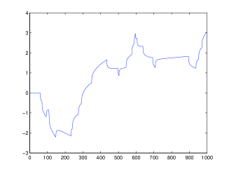
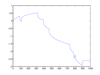
Figure 1: A path of fLpMG (left) and fLpMvN (right) with Lévy measure $\lambda(\delta_{-1}+\delta_{1})$ and $H=0.75$. The different behavior of the two processes can be seen near origin, even though the driving paths are not the same.

Figure 2: A path of fLpMG (left) and fLpMvN (right) with $H=0.25$.

Remark 3.2.

An fLpMG driven by $L$ is adapted to the natural filtration $\mathcal{F}^{L}_{t}=\sigma\{L_{u}|0\leq u\leq t\}$. This is not the case for fLpMvN.

Proposition 3.4.

An fLpMG $Y$ can be considered as the $L^{2}$- limit of approximating step functions. Moreover, the following $L^{2}$- isometry holds

$$\mathbb{E}Y_{t}^{2}=||z_{H}(t,\cdot)||^{2}_{L^{2}([0,t])}\mathbb{E}L_{1}^{2}.$$

Proof.

This is a direct consequence of Proposition 2.1. of [2]. ∎

Proposition 3.5 (Autocovariance function).

$$\mathbb{E}Y_{t}Y_{s}=\frac{\mathbb{E}L_{1}^{2}}{2}\left(t^{2H}+s^{2H}-|t-s|^{2H}\right),$$

where $s,t\geq 0$.

Proof.

By $L^{2}$- isometry we have that

$$\mathbb{E}Y_{t}^{2}=||z_{H}(t,\cdot)||^{2}_{L^{2}([0,t])}\mathbb{E}L_{1}^{2}.$$

We use the same argument for the increment (for the $L^{2}$- isometry, see [2] proposition 2.1.). Thus

$$\mathbb{E}(Y_{t}-Y_{s})^{2}=\mathbb{E}L_{1}^{2}\int_{0}^{t\vee s}(z_{H}(t,u)-z_{H}(s,u))^{2}du=\mathbb{E}L_{1}^{2}\cdot|t-s|^{2H}.$$

Now

$$\mathbb{E}Y_{t}Y_{s}=\frac{1}{2}\left(\mathbb{E}Y_{t}^{2}+\mathbb{E}Y_{s}^{2}-\mathbb{E}(Y_{t}-Y_{s})^{2}\right)=\frac{\mathbb{E}L_{1}^{2}}{2}\left(t^{2H}+s^{2H}-|t-s|^{2H}\right).$$

∎

Besides the $L^{2}$- interpretation, we have also a partial result on the pathwise construction of fLpMG.

Proposition 3.6 (Pathwise construction).

Let $H\in\left(\frac{1}{2},1\right)$ and $L$ be a compound Poisson process with characteristic triplet $(0,0,\nu)$ such that $\mathbb{E}L_{1}=0$ and $\mathbb{E}L_{1}^{2}<\infty$. Then

$$Y_{t}=\int_{0}^{t}z_{H}(t,s)dL_{s}=-\int_{0}^{t}\left(\frac{d}{ds}z_{H}(t,s)\right)L_{s}ds\quad\text{(almost surely)}.$$

Proof.

Fix $\omega\in\Omega$. A. s. there exists $\epsilon>0$ such that $L_{s}=0$ for all $s\in[0,\epsilon]$. The kernel $z_{H}(t,\cdot)$ is continuous when $s\neq 0$ by [5]. Also its derivative is continuous on $(0,t)$. We get now by Lemma 2.1. of [11] that

$$\int_{0}^{t}z_{H}(t,s)dL_{s}=\int_{\epsilon}^{t}z_{H}(t,s)dL_{s}$$

$$= z_{H}(t,t)L_{t}-z_{H}(t,\epsilon)L_{\epsilon}-\int_{\epsilon}^{t}\left(\frac{d}{ds}z_{H}(t,s)\right)L_{s}ds$$

$$= -\int_{0}^{t}\left(\frac{d}{ds}z_{H}(t,s)\right)L_{s}ds.$$

∎

The problem with the pathwise construction of fLpMG (when not in compound Poisson case) is that for $H>\frac{1}{2}$, the Molchan-Golosov kernel $z_{H}(t,\cdot)$ does not vanish at the origin like the Mandelbrot-Van Ness kernel does. However, the paths of the fLpMG are continuous when $H>\frac{1}{2}$ as is illustrated by the following theorem.

Proposition 3.7.

1. For $H>\frac{1}{2}$, an fLpMG $Y$ on $[0,T]$ has a. s. Hölder continuous paths of any order strictly less than $H-\frac{1}{2}$.

2. For $H<\frac{1}{2}$, an fLpMG $Y$ has discontinuous sample paths with positive probability.

3. For $H<\frac{1}{2}$, an fLpMG $Y$ has unbounded sample paths with positive probability.

Proof.

Let $H>\frac{1}{2}$. It holds that

$$\mathbb{E}|Y_{t}-Y_{s}|^{2}=|t-s|^{2H}=|t-s|^{1+2(H-\frac{1}{2})}.$$

The first assertion follows now from the Kolmogorov-Chentsov theorem. See for example [12].

Let now $H<\frac{1}{2}$. We know that in this case the mapping $t\mapsto z_{H}(t,s)$ is unbounded and discontinuous for all $s\in(0,T)$. Thus by theorem 4 of [13] we know that the sample paths of $Y$ are unbounded with positive probability and also discontinuous with positive probability. ∎

Remark 3.3.

Analogously one can prove that an fLpMvN has unbounded and discontinuous paths with positive probability when $H<\frac{1}{2}$.

Besides continuity, the sample paths have also the zero quadratic variation property for $H>\frac{1}{2}$. This is illustrated in the following theorem where we compute the quadratic variation over the dyadic sequence of partitions.

Theorem 3.8.

Let $(Y_{t})_{t_{\geq 0}}$ be a fLpMG with $H>\frac{1}{2}$. Then for all $t>0$ it holds that

$$\sum_{j=1}^{2^{n}}\left(Y_{\frac{j}{2^{n}}t}-Y_{\frac{j-1}{2^{n}}t}\right)^{2}\rightarrow 0\quad\text{a. s. when }n\rightarrow\infty.$$

Proof.

Set

$$V_{n}=\sum_{j=1}^{2^{n}}\left(Y_{\frac{j}{2^{n}}t}-Y_{\frac{j-1}{2^{n}}t}\right)^{2}.$$

Now we have that

$$\mathbb{E}V_{n}=(\mathbb{E}L_{1}^{2})2^{n}\left(\frac{t}{2^{n}}\right)^{2H}=(\mathbb{E}L_{1}^{2})t^{2H}2^{-n(2H-1)}.$$

We obtain using Markov inequality (see e.g. [14]) that

$$\sum_{n=1}^{\infty}\mathbb{P}\left(|V_{n}-\mathbb{E}V_{n}|\geq\frac{1}{n}\right)\leq\sum_{n=1}^{\infty}n\mathbb{E}|V_{n}-\mathbb{E}V_{n}|$$

$$\leq \sum_{n=1}^{\infty}n2\mathbb{E}V_{n}=2t^{2H}(\mathbb{E}L_{1}^{2})\sum_{n=1}^{\infty}n2^{-n(2H-1)}<\infty.$$

We use now Borel-Cantelli theorem (see [14]) and obtain that

$$V_{n}-\mathbb{E}V_{n}\rightarrow 0,\quad\text{as }n\rightarrow\infty\text{ a. s.}$$

On the other hand $\mathbb{E}V_{n}\rightarrow_{n\rightarrow\infty}0$. Thus $V_{n}\rightarrow_{n\rightarrow\infty}0$ a. s. ∎

Note that the same proof works also in the case of fLpMvN. Thus, we have the following theorem.

Theorem 3.9.

Let $X$ be an fLpMvN with $H>\frac{1}{2}$. Then for $-\infty<s<t<\infty$ it holds that

$$\sum_{j=1}^{2^{n}}\left(X_{s+\frac{j}{2^{n}}(t-s)}-X_{s+\frac{j-1}{2^{n}}(t-s)}\right)^{2}\rightarrow 0\quad\text{a.s. when }n\rightarrow\infty.$$

Proposition 3.10 (Characteristic function).

Let $u_{1},\dots,u_{n}\in\mathbb{R}$ and $0<t_{1}<\dots<t_{n}<\infty$. Then

$$\mathbb{E}\left(\exp\left(i\sum_{j=1}^{n}u_{j}Y_{t_{j}}\right)\right)=\exp\left(\int_{\mathbb{R}}\Psi\left(\sum_{j=1}^{n}u_{j}z_{H}(t_{j},s)\right)ds\right),$$

where $\Psi$ is the characteristic exponent of the driving Lévy process $L$. Moreover, $Y_{t}$ is infinitely divisible for all $t\geq 0$.

Proof.

This follows, for example, from [10]. ∎

Proposition 3.11.

The increments of fLpMG are not always stationary.

Proof.

Consider fLpMG $Y$ driven by a compound Poisson process $L$ with Lévy measure $\nu=\frac{1}{2}(\delta_{1}+\delta_{-1})$, where $\delta_{\cdot}$ denotes the Dirac delta. For $\epsilon>0$

$$\mathbb{P}(Y_{\epsilon}-Y_{0}=0)\geq\mathbb{P}(L_{t}=0\quad\forall t\leq\epsilon)=1-e^{-\epsilon}.$$

On the other hand, consider set

$$A=\{\omega\in\Omega\text{ s.t. }\#\{s\in[0,1]\text{ s.t. }\Delta L_{s}\neq 0\}=1\text{ and }\#\{s\in(1,\epsilon]\text{ s.t. }\Delta L_{s}\neq 0\}=0\}.$$

In set $A$, there is one jump time $S\in[0,1]$ and $\Delta L_{S}=\pm 1$. It follows that

$$Y_{1+\epsilon}-Y_{1}=\left(\frac{d}{ds}z_{H}(1+\epsilon,s)-\frac{d}{ds}z_{H}(1,s)\right)_{s=S}\Delta L_{S}\neq 0,$$

by proposition 3.6. We also have that

$$\mathbb{P}(Y_{1+\epsilon}-Y_{1}=0)\leq 1-\mathbb{P}(A)=1-e^{-1}(1-e^{-\epsilon})<1-e^{-\epsilon},$$

when $\epsilon>0$ small enough. Thus, $Y_{\epsilon}-Y_{0}\stackrel{{\scriptstyle d}}{{\neq}}Y_{1+\epsilon}-Y_{1}$. Hence, the increments of fLpMG $Y$ are not stationary. ∎

Theorem 3.12 (Self-similarity).

Fractional Lévy process by Molchan-Golosov transformation cannot be self-similar for $H\in(0,1)$.

Proof.

Assume that the process $Y$ is self-similar with some index $\alpha$. Then we have for all $c>0$ that

$$\left(Y_{ct}\right)_{t\geq 0}\stackrel{{\scriptstyle d}}{{=}}\left(c^{\alpha}Y_{t}\right)_{t\geq 0}.$$

The characteristic function of $Y$ is given by theorem 3.10. On the other hand

$$\mathbb{E}e^{iuY_{t}}=\mathbb{E}e^{iuc^{-\alpha}Y_{ct}}$$

$$= \exp\left(\int_{0}^{ct}\int_{\mathbb{R}}\left(e^{ic^{-\alpha}uxz_{H}(ct,s)}-1-ic^{-\alpha}uxz_{H}(ct,s)\right)\nu(dx)ds\right)$$

$$= \exp\left(\int_{0}^{t}\int_{\mathbb{R}}\left(e^{ic^{-\alpha}c^{H-\frac{1}{2}}uxz_{H}(t,s)}-1-ic^{-\alpha}c^{H-\frac{1}{2}}uxz_{H}(t,s)\right)\nu(dx)cds\right)$$

$$= \exp\left(\int_{0}^{t}\int_{\mathbb{R}}\left(e^{iuxz_{H}(t,s)}-1-iuxz_{H}(t,s)\right)c\nu\left(c^{\alpha-H+\frac{1}{2}}dx\right)ds\right).$$

Note that $\alpha-H+\frac{1}{2}=0$ implies that $Y\stackrel{{\scriptstyle d}}{{=}}cY$ for all $c>0$ which means that $Y=L=0$ identically. We define for $r>0$ the translation operator $T_{r}$ of measures on $\mathbb{R}$ for $B\in\mathcal{B}(\mathbb{R})$ by

$$(T_{r}\nu)(B)=\nu\left(r^{-1}B\right).$$

Now the Lévy measure of infinitely divisible random variable $c^{-\alpha}Y_{ct}$ is given by $cT_{r}\nu_{Y_{t}}$, where $r=c^{-H+\frac{1}{2}+\alpha}$ and

$$\nu_{Y_{t}}(B)=\int_{0}^{t}\int_{\mathbb{R}}1_{B}\left(z_{H}(t,s)x\right)\nu(dx)ds.$$

The drift parameter of $Y_{1}$ is $\gamma_{Y_{1}}$. It follows from the uniqueness of the generating triplet and self-similarity property that it holds for all $b>0$

$$\nu_{Y_{t}}=b^{1/\left(H-\frac{1}{2}-\alpha\right)}T_{b}\nu_{Y_{t}}.$$

Denote now $\beta=\frac{-1}{H-\frac{1}{2}-\alpha}$. Let $\mu$ be the distribution of random variable $Y_{1}$ and let $\hat{\mu}(u)$ be the characteristic function of $\mu$. Random variable $bY_{1}$ has now characteristic function $\hat{\mu}(bu)$. Because $Y_{1}$ is infinitely divisible, we can use proposition 11.10 of [8] that the triplet of $bY_{1}$ is $(\gamma(b),0,T_{b}\nu_{Y_{1}})$ for some $\gamma(b)$. On the other hand, $\hat{\mu}(u)^{b^{\beta}}$ is an infinitely divisible characteristic function with triplet $(b^{\beta}\gamma_{Y_{1}},0,b^{\beta}\nu_{Y_{1}})$. Thus we have for any $b>0$ some $d$ such that

$$\hat{\mu}(u)^{a}=\hat{\mu}(bu)e^{idu},$$

where $a=b^{\beta}$. We note that $\mathbb{R}_{+}\mapsto\mathbb{R}_{+}:b\mapsto b^{\beta}$ is one-to-one. Thus, $\mu$ follows a stable law with index $\beta$. The index $\beta\in(0,2]$ by definition 13.5. of [8]. By theorem 14.1. of [8], $\beta=2$ corresponds to Gaussian case and is thus impossible. It follows now that $\mathbb{E}Y_{t}^{2}=\infty$, which contradicts the fact that $Y_{t}\in L^{2}(\Omega,\mathbb{P})$. Thus, fLpMG can never be self-similar of any order $\alpha$. ∎

Remark 3.4.

In [3], the authors define fractional subordinators by Molchan-Golosov transformation using pathwise Riemann-Stieltjes integration. However, these processes are not fLpMG as considered here, since subordinators are increasing Lévy processes and here we consider only zero mean Lévy processes. Also the integration concept there is different.

4 Relation of the two fLp concepts

The connection between fractional Lévy processes by Molchan-Golosov transformation and Mandelbrot-Van Ness transformation is basically the same as in the fBm case. The result in fLp case is new.

Let $H\in\left(0,1\right)$ and $L$ be a two-sided Lévy process without Brownian component satisfying $\mathbb{E}L_{1}=0$ and $\mathbb{E}L_{1}^{2}<\infty$. Let $s>0$ and set

$$Y^{s}_{t}=\int_{0}^{t}z_{H}(t,u)dL_{u-s}=c_{H}\int_{0}^{t}(t-u)^{H-\frac{1}{2}}\tilde{F}\left(\frac{u-t}{u}\right)dL_{u-s},\quad t\in[0,\infty),$$

which is in fact fLpMG with Hurst parameter $H$. Here

$$\tilde{F}(x)=F\left(\frac{1}{2}-H,H-\frac{1}{2},H+\frac{1}{2},x\right),$$

where $F$ is the Gauss’ hypergeometric function. Define the time shifted process

$$Z^{s}_{t}=Y^{s}_{t+s}-Y^{s}_{s},\quad t\in[-s,\infty).$$

In the fBm case this would also be fBm, but in fLpMG case we do not have the stationarity of the increments and we are lacking such an interpretation. Now we substitute $v=u-s$ and obtain a.s. that

$$Z^{s}_{t}=c_{H}\left(\int_{-s}^{t}(t-v)^{H-\frac{1}{2}}\tilde{F}\left(\frac{v-t}{v+s}\right)dL_{v}-\int_{-s}^{0}(-v)^{H-\frac{1}{2}}\tilde{F}\left(\frac{v}{v+s}\right)dL_{v}\right).$$

By [15], $\tilde{F}(0)=1$ and thus we obtain formally as $s\rightarrow\infty$ that

$$Z^{\infty}_{t}:=\frac{c_{H}}{C_{H}}X_{t}:=c_{H}\int_{\mathbb{R}}\left((t-v)_{+}^{H-\frac{1}{2}}-(-v)_{+}^{H-\frac{1}{2}}\right)dL_{v},\quad t\in\mathbb{R}.$$

Theorem 4.1.

For every $t\in\mathbb{R}$ there exist constants $S,C>0$ such that

$$\mathbb{E}\left(Z^{s}_{t}-Z^{\infty}_{t}\right)^{2}\leq Cs^{2H-2},\quad\text{for }s>S.$$

Proof.

We obtain

$$\frac{1}{c_{H}^{2}\mathbb{E}L_{1}^{2}}\mathbb{E}\left(Z^{s}_{t}-Z^{\infty}_{t}\right)^{2}$$

$$= \int_{\mathbb{R}}\left(\left((t-v)^{H-\frac{1}{2}}-(-v)^{H-\frac{1}{2}}\right)1_{(-\infty,-s)}(v)\right)^{2}dv$$

$$+ \int_{\mathbb{R}}\left((t-v)^{H-\frac{1}{2}}\left(\tilde{F}\left(\frac{v-t}{v+s}\right)-1\right)1_{(-s,t)}(v)\right.$$

$$- \left.(-v)^{H-\frac{1}{2}}\left(\tilde{F}\left(\frac{v}{v+s}\right)-1\right)1_{(-s,0)}(v)\right)^{2}dv,$$

by $L^{2}$- isometry and independence of increments of $L$. The claim follows now from the proof of Theorem 3.1. of [15]. ∎

5 Wiener integration

Here our goal is to define suitable Wiener integrals with respect to fLpMG. In contrary to the case of fLpMvN, we use the fractional integration on a compact interval instead of the whole real line. We will define the space $L^{2}_{H}([0,T])$ of integrands as in the case of compact interval Wiener integrals in fBm case.

Let $g$ be a function defined on $[0,T]$ and $I_{-}^{H-\frac{1}{2}}$ be the right-sided Riemann-Liouville integral operator of order $H-\frac{1}{2}$ as in [5]. Define operator

$$(K^{H}g)(s)=\Gamma(H+\frac{1}{2})c_{H}s^{\frac{1}{2}-H}\left(I_{-}^{H-\frac{1}{2}}\left((\cdot)^{H-\frac{1}{2}}g(\cdot)\right)\right)(s),\quad s,t\in[0,T].$$

Now it holds by [5] that

$$z_{H}(t,s)=\Gamma(H+\frac{1}{2})c_{H}s^{\frac{1}{2}-H}\left(I_{-}^{H-\frac{1}{2}}(\cdot)^{H-\frac{1}{2}}1_{[0,t)}\right)(s),$$

for $0\leq t\leq T$. Define now the space

$$L_{H}^{2}([0,T])=\{g\in L^{1}([0,T])|K^{H}g\in L^{2}([0,T])\},$$

equipped with norm $||g||_{L_{H}^{2}([0,T])}:=||K^{H}g||_{L^{2}([0,T])}$. Now we are ready for the definition of Wiener integral.

Definition 5.1 (Wiener integral for fLpMG).

Let $H\in(0,1)$, $Y$ be a fLpMG driven by Lévy process $L$. For $g\in L^{2}_{H}([0,T])$ the Wiener integral with respect to fLpMG is defined as

$$\int_{0}^{T}g(s)dY_{s}=\int_{0}^{T}(K^{H}g)(s)dL_{s}.$$

Note that the definition is completely analogous to the definition of compact interval Wiener integrals in the fBm setup. Now, let $g$ be a step function, which means that

$$g(s)=\sum_{j=1}^{n}a_{j}1_{(s_{j-1},s_{j}]}(s),$$ (1)

where $a_{0},\dots,a_{n}\in\mathbb{R}$ and $0=s_{0}<s_{1}<\dots<s_{n}=T$. Now $g\in{L}^{2}_{H}([0,T])$ and we have the following result.

Lemma 5.2.

Assume $H\in(0,1)$, $Y$ is fLpMG driven by $L$ and $g$ a step function defined by equation (1). It holds that

$$\int_{0}^{T}g(s)dY_{s}=\sum_{j=1}^{n}a_{j}\left(Y_{s_{j}}-Y_{s_{j-1}}\right).$$

Proof.

It is clear from the definition that the integral of a step function is linear. We will prove the claim for indicator functions. The general claim follows from the linearity. Set $g(s)=1_{(s_{1},s_{2}]}$. Now

$$\int_{0}^{T}g(s)dY_{s}=\int_{0}^{T}\left(K^{H}g\right)(s)dL_{s}=\int_{0}^{T}\left(K^{H}\left(1_{(0,s_{2}]}-1_{(0,s_{1}]}\right)\right)(s)dL_{s}$$

$$= Y_{s_{2}}-Y_{s_{1}}.$$

∎

Obviously the following isometry holds for a step function $g$

$$||\int_{0}^{T}(K^{H}g)(s)dL_{s}||_{L^{2}(\mathbb{P})}^{2}=\mathbb{E}L_{1}^{2}\int_{0}^{T}(K^{H}g)^{2}(s)ds=\mathbb{E}L_{1}^{2}\cdot||g||^{2}_{{L}^{2}_{H}([0,T])}.$$ (2)

Next we restrict ourselves to the case $H\in\left(0,\frac{1}{2}\right)$. In this case $L^{2}_{H}([0,T])$ is complete ([16]) and the step functions are dense in $L^{2}_{H}([0,T])$. Thus we can make the following alternative definition. Note that both the definitions yield the same Wiener integral.

Definition 5.3.

Let $Y$ be a fLpMG with driving Lévy process $L$ and Hurst index $H\in\left(0,\frac{1}{2}\right)$. Let $g\in L^{2}_{H}([0,T])$ and let $\{g_{k}\}_{k\in\mathbb{Z}_{+}}$ be a sequence of step functions converging to $g$ in $L^{2}_{H}([0,T])$. We define the Wiener integral of $g$ with respect to $Y$ as follows

$$\int_{0}^{T}g(s)dY_{s}=L^{2}(\mathbb{P})-\lim_{k\rightarrow\infty}\int_{0}^{T}g_{k}(s)dY_{s}.$$

Note that the definition does not depend on the approximating sequence.

6 Financial application

Next we will construct an arbitrage free model including fractional Lévy processes. This is a (geometric) mixed Brownian motion and fractional Lévy process model. The no-arbitrage result is analogous to the result in the case of mixed Brownian motion and fractional Brownian motion.

In the following, $Z$ may be either fLpMG or fLpMvN with $H>\frac{1}{2}$ and $W$ is an ordinary Brownian motion independent of $Z$. Let $\sigma,\epsilon>0$. Define the mixed process by

$$U_{t}=\sigma Z_{t}+\epsilon W_{t}.$$ (3)

Theorem 6.1.

Let the market model be given by $(\Omega,\mathcal{F},\exp{U},(\mathcal{F}_{t}^{U}),\mathbb{P})$ and let $\Phi$ be a stopping-smooth trading strategy, where we use the conventions of [17]. Then $\Phi$ is not an arbitrage opportunity.

Proof.

We will check the assumptions of Theorem 5 of [17] and then we are done. The two conditions to be checked, are the quadratic variation property and the conditional small ball property.

Both fLpMvN and fLpMG are continuous path processes with zero quadratic variation over the dyadic partitions, see Theorems 3.8 and 3.9. Thus $U$ has the quadratic variation of Brownian motion over these partitions.

Moreover, $U$ has conditional full support (CFS) w.r.t. its own filtration by Theorem 3.1  of [18]. Since $U$ has CFS w.r.t. $(\mathcal{F}^{U}_{t})$ on $\mathbb{R}$, it follows that $\exp{U}$ has CFS w.r.t. $(\mathcal{F}^{U}_{t})$ on $\mathbb{R}_{+}$. This is equivalent to the conditional small ball property of [17] by Lemma 2.3  of [18]. ∎

The exact definition for stopping-smooth strategies is not given in this paper, because it is rather technical. According to [17] the chosen strategies cover hedges for many European, lookback and Asian options. Thus, it is an economically meaningful class.

This mixed model is a natural way for modeling shocks in financial markets. The Brownian motion part corresponds to the ordinary noise in the market and the fractional Lévy process part to sudden shocks in the market. On the other hand the fractional Lévy process has the covariance structure of fBm, this allows to model for long-range dependence.

The no-arbitrage result holds for both fLp concepts, but from the modeling point of view they are different. If one wants to have stationary increments of $U$, one should use fLpMvN. If one wants to avoid history from $-\infty$, one should use fLpMG instead. In real world, there is always the time $0$ when the trading began. Hence fLpMG might be more natural choice. However, this modeling question is rather delicate.

If in the model (3), $Z$ is of bounded variation, then $U$ is a semimartingale with Brownian motion as the martingale part of the decomposition. However, this model has long-range dependence property.

7 Proofs

First we prove a lemma about the connection of the normalizing constants of the different integral representations.

Lemma 7.1.

For any $H\in(0,1)$

$$C_{H}=c_{H}.$$

Proof.

First of all by [19]

$$C_{H}=\frac{(2H\sin{(\pi H)}\Gamma{(2H)})^{\frac{1}{2}}}{\Gamma{(H+\frac{1}{2})}}.$$

Now we have that

$$C_{H}-c_{H}=\frac{1}{\Gamma(H+\frac{1}{2})}\left((2H\sin{(\pi H)}\Gamma(2H))^{\frac{1}{2}}-\left(\frac{2H\Gamma(H+\frac{1}{2})\Gamma(\frac{3}{2}-H)}{\Gamma(2-2H)}\right)^{\frac{1}{2}}\right)$$

$$= \frac{1}{\Gamma(H+\frac{1}{2})}\sqrt{\frac{2H}{\Gamma(2-2H)}}\left((\sin{(\pi H)}\Gamma(2H)\Gamma(2-2H))^{\frac{1}{2}}-(\Gamma(H+\frac{1}{2})\Gamma(\frac{3}{2}-H))^{\frac{1}{2}}\right).$$

For the difference we have now that

$$(\sin{(\pi H)}\Gamma(2H)\Gamma(2-2H))^{\frac{1}{2}}-(\Gamma(H+\frac{1}{2})\Gamma(\frac{3}{2}-H))^{\frac{1}{2}}$$

$$= (\sin{(\pi H)}(2H-1)\Gamma(2H-1)\Gamma(2-2H))^{\frac{1}{2}}-((H-\frac{1}{2})\Gamma(H-\frac{1}{2})\Gamma(\frac{3}{2}-H))^{\frac{1}{2}}$$

$$= \sqrt{H-\frac{1}{2}}\left(\left(2\sin{(\pi H)}\frac{\pi}{\sin{\pi(2H-1)}}\right)^{\frac{1}{2}}-\left(\frac{\pi}{\sin{\pi(H-\frac{1}{2})}}\right)^{\frac{1}{2}}\right)$$

$$= \sqrt{\pi(H-\frac{1}{2})}\left(\left(-\frac{2\sin{(\pi H)}}{\sin{(2\pi H)}}\right)^{\frac{1}{2}}-\left(\frac{-1}{\cos{\pi H}}\right)^{\frac{1}{2}}\right)$$

$$= \sqrt{\pi(H-\frac{1}{2})\sin{2\pi H}\cos{(\pi H)}}\left((-2\sin{(\pi H)\cos{(\pi H)}})^{\frac{1}{2}}-(-\sin(2\pi H))^{\frac{1}{2}}\right)=0.$$

The previous computation is for $H>\frac{1}{2}$, but an analogous computation goes through for $H<\frac{1}{2}$ as well. ∎

Next we present some results about finiteness of the moments of different kernels.

Lemma 7.2.

Let $H>\frac{1}{2}$ and $K>2$. Then for any $t>0$

$$\int_{0}^{t}(z_{H}(t,s))^{K}ds=\infty,$$

when $H\geq\frac{1}{2}+\frac{1}{K}$.

Proof.

$$(H-\frac{1}{2})^{-K}c_{H}^{-K}\int_{0}^{t}(z_{H}(t,s))^{K}ds=\int_{0}^{t}s^{K(\frac{1}{2}-H)}\left(\int_{s}^{t}u^{H-\frac{1}{2}}(u-s)^{H-\frac{3}{2}}du\right)^{K}ds$$

$$\geq \int_{0}^{t}s^{K(\frac{1}{2}-H)}\left(\int_{s}^{t}(u-s)^{H-\frac{1}{2}}(u-s)^{H-\frac{3}{2}}\right)^{K}ds$$

$$= \int_{0}^{t}s^{K(\frac{1}{2}-H)}\left(\frac{1}{2H-1}(t-s)^{2H-1}\right)^{K}ds.$$

We note that the factor

$$\left(\frac{1}{2H-1}(t-s)^{2H-1}\right)^{K}$$

is bounded and also bounded away from zero in some neighborhood of the origin. Thus the last integral is finite if and only if

$$\int_{0}^{t}s^{K(\frac{1}{2}-H)}ds<\infty.$$

Thus the integral $\int_{0}^{t}(z_{H}(t,s))^{K}ds=\infty$ if $K(\frac{1}{2}-H)\leq 1$ i.e. $H\geq\frac{1}{2}+\frac{1}{K}$. ∎

Lemma 7.3.

For $H>\frac{1}{2}$ and any $t>0$

$$\int_{-\infty}^{t}(f_{H}(t,s))^{K}ds<\infty,\quad K\geq 2.$$

Proof.

From self-similarity, is sufficient to consider only $t=1$. We have that

$$C_{H}^{-K}\int_{0}^{1}(f_{H}(1,s))^{K}ds=\int_{-\infty}^{0}\left((1-s)^{H-\frac{1}{2}}-(-s)^{H-\frac{1}{2}}\right)^{K}ds+\frac{1}{K(H-\frac{1}{2})+1}.$$

For the first term we get

$$\int_{-\infty}^{0}\left((1-s)^{H-\frac{1}{2}}-(-s)^{H-\frac{1}{2}}\right)^{K}ds=\int_{0}^{\infty}\Big{(}(1+s)^{H-\frac{1}{2}}-s^{H-\frac{1}{2}}\Big{)}^{K}ds$$

$$= \int_{0}^{1}z^{K(\frac{1}{2}-H)}((1+z)^{H-\frac{1}{2}}-1)^{K}z^{-2}dz=\int_{0}^{1}z^{K(\frac{1}{2}-H)-2}((1+z)^{H-\frac{1}{2}}-1)^{K}dz.$$

By the Lagrange theorem we have that for some $x\in[0,z]$

$$(1+z)^{H-\frac{1}{2}}-1=\Big{(}H-\frac{1}{2}\Big{)}(1+x)^{H-\frac{3}{2}}z\leq\Big{(}H-\frac{1}{2}\Big{)}z.$$

Now we have that

$$\int_{0}^{1}z^{K(\frac{1}{2}-H)-2}((1+z)^{H-\frac{1}{2}}-1)^{K}dz\leq\Big{(}H-\frac{1}{2}\Big{)}^{K}\int_{0}^{1}z^{K(\frac{1}{2}-H)-2}z^{K}dz$$

$$= \Big{(}H-\frac{1}{2}\Big{)}^{K}\int_{0}^{1}z^{K(\frac{3}{2}-H)-2}dz<\infty,$$

since $K\left(\frac{3}{2}-H\right)-2>2\left(\frac{3}{2}-1\right)-2=-1.$

∎

Remark 7.1.

It follows from two above lemmas that for any $H\geq\frac{1}{2}+\frac{1}{K}$ and $t>0$ we have inequality $\int_{-\infty}^{t}(f_{H}(t,s))^{K}ds<\int_{0}^{t}(z_{H}(t,s))^{K}ds$.

Now we want to establish similar inequalities for $K=3,4$ and $\frac{1}{2}<H<\frac{1}{2}+\frac{1}{K}$.

Lemma 7.4.

1) For any $\frac{1}{2}<H<\frac{5}{6}$ and any $t>0$ we have the inequality

$\int_{-\infty}^{t}(f_{H}(t,s))^{3}ds<\int_{0}^{t}(z_{H}(t,s))^{3}ds$.

2) For any $\frac{1}{2}<H<\frac{3}{4}$ and any $t>0$ we have the inequality

$\int_{-\infty}^{t}(f_{H}(t,s))^{4}ds<\int_{0}^{t}(z_{H}(t,s))^{4}ds$.

Proof.

The proof is similar in both the cases so consider the first one. It is better to normalize the integrals, and for the normalized Molchan-Golosov kernel we obtain that

$$\frac{1}{C_{H}^{3}}\int_{0}^{1}(z_{H}(1,s))^{3}ds$$

$$= \Big{(}H-\frac{1}{2}\Big{)}^{3}\int_{0}^{1}s^{\frac{3}{2}-3H}\left(\int_{s}^{1}u^{H-\frac{1}{2}}(u-s)^{H-\frac{3}{2}}du\right)^{3}ds.$$

Note that integration by parts leads to the equality

$$\Big{(}H-\frac{1}{2}\Big{)}\int_{s}^{1}u^{H-\frac{1}{2}}(u-s)^{H-\frac{3}{2}}du=(1-s)^{H-\frac{1}{2}}-\Big{(}H-\frac{1}{2}\Big{)}\int_{s}^{1}u^{H-\frac{3}{2}}(u-s)^{H-\frac{1}{2}}du.$$

Further, for $s\leq u\leq 1$ we have that

$$(u-s)^{H-\frac{1}{2}}=u^{H-\frac{1}{2}}\Big{(}1-\frac{s}{u}\Big{)}^{H-\frac{1}{2}}\leq u^{H-\frac{1}{2}}(1-s)^{H-\frac{1}{2}},$$

whence

$$(1-s)^{H-\frac{1}{2}}-\Big{(}H-\frac{1}{2}\Big{)}\int_{s}^{1}u^{H-\frac{3}{2}}(u-s)^{H-\frac{1}{2}}du$$

$$\geq (1-s)^{H-\frac{1}{2}}\Big{(}1-\Big{(}H-\frac{1}{2}\Big{)}\int_{s}^{1}u^{2H-2}du\Big{)}=\frac{1}{2}(1-s)^{H-\frac{1}{2}}(1+s^{2H-1}).$$

Denote $p=H-\frac{1}{2},\,\frac{1}{2}<H<\frac{5}{6}$ and $\alpha_{p}^{1}=\frac{1}{C_{H}^{3}}\int_{0}^{1}(z_{H}(1,s))^{3}ds.$ Then $p\in(0,\frac{1}{3})$ and we obtain from previous estimates that

$$\alpha_{p}^{1}\geq\frac{1}{8}\int_{0}^{1}s^{-3p}(1-s)^{3p}(1+s^{2p})^{3}ds$$

$$= \int_{0}^{1}s^{-3p}(1-s)^{3p}s^{3p}ds+\frac{1}{8}\int_{0}^{1}s^{-3p}(1-s)^{3p}((1+s^{2p})^{3}-8s^{3p})ds$$

$$=\int_{0}^{1}(1-s)^{3p}ds+\frac{1}{2}\int_{0}^{1}s^{-3p}(1-s)^{3p}(1-s^{p})^{2}\Big{(}\frac{1+2s^{2p}+s^{4p}}{4}+\frac{s^{p}+s^{3p}}{2}+s^{2p}\Big{)}ds$$

$$=:\alpha_{p}^{11}+\alpha_{p}^{12}.$$

Evidently, $\alpha_{p}^{11}=\frac{1}{3p+1}$. For $\alpha_{p}^{12}$ we use the following simple bounds: on the interval $s\in[0,1]$ $1\geq s^{kp},k=1,2,3,4$ and for $p\in(0,\frac{1}{3}),\,s\in[0,1]$ $(1-s)^{3p}\geq 1-s^{3p}.$

Therefore,

$$\alpha_{p}^{12}\geq\frac{3}{2}\int_{0}^{1}s^{p}(1-s^{3p})(1-s^{p})^{2}ds$$

$$=\frac{3}{2}\int_{0}^{1}(s^{p}-2s^{2p}+s^{3p}-s^{4p}+2s^{5p}-s^{6p})ds$$

$$=\frac{3}{2}\Big{(}\frac{1}{p+1}-\frac{2}{2p+1}+\frac{1}{3p+1}-\frac{1}{4p+1}+\frac{2}{5p+1}-\frac{1}{6p+1}\Big{)}$$

$$=9p^{3}\frac{38p^{2}+21p+3}{\prod_{k=1}^{6}(kp+1)}.$$

On the other hand, for the normalized Mandelbrot-Van Ness kernel we can use the same reasonings as in the proof of Lemma 7.3 and obtain in the above notations that

$$\alpha_{p}^{2}:=C_{H}^{-3}\int_{0}^{1}(f_{H}(1,s))^{3}ds$$

$$=\int_{-\infty}^{0}\left((1-s)^{p}-(-s)^{p}\right)^{3}ds+\frac{1}{3p+1}$$

$$=\int_{0}^{1}s^{-3p-2}((1+s)^{p}-1)^{3}ds+\frac{1}{3p+1}$$

$$\leq p^{3}\int_{0}^{1}s^{-3p+1}ds+\frac{1}{3p+1}=\frac{p^{3}}{2-3p}+\frac{1}{3p+1}.$$

To establish the inequality $\alpha_{p}^{1}>\alpha_{p}^{2}$, that is equivalent to the statement of the lemma, it is sufficient to prove that

$$9p^{3}\frac{38p^{2}+21p+3}{\prod_{k=1}^{6}(kp+1)}>\frac{p^{3}}{2-3p},\,p\in\Big{(}0,\frac{1}{3}\Big{)},$$

or

$$9\frac{38p^{2}+21p+3}{\prod_{k=1}^{6}(kp+1)}>\frac{1}{2-3p},\,p\in\Big{(}0,\frac{1}{3}\Big{)}.$$

For technical simplicity, diminish the left-hand side and compare the functions $f_{1}(p)=9\frac{36p^{2}+21p+3}{\prod_{k=1}^{6}(kp+1)}=27\frac{12p^{2}+7p+1}{\prod_{k=1}^{6}(kp+1)}$ and $f_{2}(p)=\frac{1}{2-3p}$. Of course, to finish the proof, it is sufficient to establish the inequality$f_{1}(p)\geq f_{2}(p),\,p\in(0,\frac{1}{3})$.

Note that $f_{2}(p)$ increases from $\frac{1}{2}$ to $1$. The derivative of $f_{1}(p)$ can be estimated, up to positive multiplier, as

$$(24p+7)\prod_{k=1}^{6}(kp+1)-(12p^{2}+7p+1)\sum_{r=1}^{6}r\prod_{k=1,k\neq r}^{6}(kp+1)$$

$$\leq\prod_{k=1}^{5}(kp+1)((24p+7)(6p+1)-21(12p^{2}+7p+1))$$

$$=-\prod_{k=1}^{5}(kp+1)(108p^{2}+81p+14)<0.$$

It means that $f_{1}(p)$ decreases on $(0,\frac{1}{3}),$ and it decreases from $27$ to $\frac{243}{160}>1$ that completes the proof. ∎

Remark 7.2.

The integral with respect to Molchan–Golosov kernel can be bounded from below in terms of Beta- or Gamma-functions. These estimates are more sharp that obtained in the proof of Lemma 7.4; however, we can not proceed with them otherwise than numerically. Indeed, for example, in the case $K=4$ we can estimate

$$\frac{1}{C_{H}^{4}}\int_{0}^{1}(z_{H}(1,s))^{4}ds\geq\frac{1}{16}\int_{0}^{1}s^{-4p}(1-s)^{4p}(1+s^{2p})^{4}ds$$

$$=\frac{1}{16}B(3-4H,4H-1)+\frac{1}{4}B(2-2H,4H-1)+\frac{1}{4}B(2H,4H-1)$$

$$+\frac{1}{16}B(4H-1,4H-1)+\frac{3}{8}\frac{1}{4H-1}=:g_{1}(p).$$

As before, $\frac{1}{c_{H}^{4}}\int_{0}^{1}(f_{H}(1,s))^{4}ds\leq\frac{p^{4}}{5-4p}+\frac{1}{4p+1}=g_{2}(p).$ The difference $g_{1}(p)-g_{2}(p),p=H-\frac{1}{2},$ is presented on Figure 3 in terms of Hurst parameter $H$.

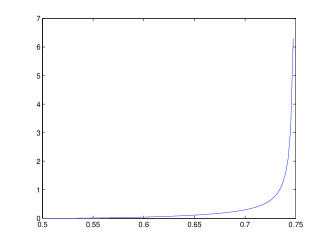
Figure 3: The difference of for the integrals of Molchan-Golosov and Mandelbrot-van-Ness kernels for $K=4$ as the function of $H$.

Now we are ready for the proof of the main result, i.e., Theorem 3.2.

Proof.

With assumptions $\mathbb{E}L_{1}=0$ and $\mathbb{E}L_{1}^{2}<\infty$ we can write the characteristic exponent of the driving Lévy process as follows

$$\Psi(t)=-\frac{1}{2}\sigma^{2}u^{2}+\int_{\mathbb{R}}\left(e^{iux}-1-iux\right)\nu(dx).$$

Prove only the second statement, the first one can be proved in a similar way. We use the representation formula for the characteristic function of fractional Lévy process and get that the fourth cumulant of the fLpMG $Y$ is given by

$$\int_{0}^{t}(z_{H}(t,s))^{4}ds\int_{\mathbb{R}}x^{4}\nu(dx).$$

Analogously the fourth cumulant of the fLpMvN $X$ is

$$\int_{-\infty}^{t}(f_{H}(t,s))^{4}ds\int_{\mathbb{R}}x^{4}\nu(dx).$$

Note that iff the Lévy measure $\nu$ is nondegenerate, $\int_{\mathbb{R}}x^{4}\nu(dx)>0$.

Our aim is now to prove that with the assumption $\mathbb{E}L_{1}^{4}<\infty$ the fourth cumulants of different fLp’s are different. This will prove that the different fractional Lévy processes have different distributions.

For $H\geq\frac{3}{4}$ the 4th cumulant of fLpMG $Y$ is infinite by lemma 7.2. On the other hand the corresponding cumulant for fLpMvN $X$ is finite by lemma 7.3.

The case $H\in(\frac{1}{2},\frac{3}{4})$ uses Lemma 7.4, and we immediately obtain the proof. ∎

Next we proof Proposition 3.3.

Proof.

Let $L$ be a compound Poisson process with parameter $\lambda$ s.t. $\mathbb{E}L_{1}=0$ and $\mathbb{E}L^{2}_{1}<\infty$. We have for fLpMG $Y$ by proposition 3.6 $\mathbb{P}(Y_{t}=0)\geq e^{-\lambda t}$ for $t>0$. On the other hand, for $t>0$ we can decompose fLpMvN $X$ to two independent components

$$\int_{-\infty}^{-1}f_{H}(t,s)dL_{s}+\int_{-1}^{t}f_{H}(t,s)dL_{s}.$$

Probability that $L$ jumps exactly once on $[-1,t)$ is $\lambda(1+t)e^{-\lambda(1+t)}$ and probability that $L$ does not have jumps on $[-1,t)$ is $e^{-\lambda(1+t)}$. Now it is easy to see that

$$\mathbb{P}(X_{t}=0)\leq\lambda(1+t)e^{-\lambda(1+t)}\wedge e^{-\lambda(1+t)}<e^{-\lambda t}\leq\mathbb{P}(Y_{t}=0)$$

for $t>0$ small enough. ∎

References

- [1] Benassi, A., Cohen, S., and Istas, J. 2004. On roughness indices for fractional fields. Bernoulli 10(2):357–373.
- [2] Marquardt, T. 2006. Fractional Lévy processes with an application to long memory moving average processes. Bernoulli 12(6):1099–1126.
- [3] Bender, C., and Marquardt, T. 2009. Integrating volatility clustering into exponential Lévy models. J. Appl. Probab. 46(3):609–628.
- [4] Samorodnitsky, G., and Taqqu, M.S. 1994. Stable non-Gaussian random processes, Chapman & Hall, Boca Raton.
- [5] Jost, C. 2007. Integral Transformations of Volterra Gaussian Processes, PhD Thesis, University of Helsinki, Helsinki.
- [6] Nualart, D. 2006. The Malliavin Calculus and Related Topics, Springer, Berlin.
- [7] Kyprianou, A.E. 2006. Introductory Lectures on Fluctuations of Lévy Processes with Applications, Springer, Berlin.
- [8] Sato, K.-I. 1999. Lévy Processes and Infinitely Divisible Distributions, Cambridge University Press, Cambridge.
- [9] Bender, C., and Marquardt, T. 2008. Stochastic calculus for convoluted Lévy processes. Bernoulli 14(2):499–518.
- [10] Rajput, B.S., and Rosinski, J. 1989. Spectral representations of infinitely divisible processes. Probab. Th. Rel. Fields 82:451–487.
- [11] Eberlein, E., and Raible S. 1999. Term structure models driven by general Lévy processes. Math. Finance 9(1):31–53.
- [12] Karatzas I., and Shreve, S.E. 1998. Brownian Motion and Stochastic Calculus. Springer, New York.
- [13] Rosinski, J. 1989. On path properties of certain infinitely divisible processes. Stochastic Process. Appl. 33:73–87.
- [14] Jacod, J., and Protter, P. 2004. Probability Essentials. Springer, Berlin.
- [15] Jost, C. 2008. On the connection between Molchan-Golosov and Mandelbrot-Van Ness representations of fractional Brownian motion. J. Integral Equations Appl. 20(1):93–119.
- [16] Sottinen, T. 2003. Fractional Brownian motion in finance and queuing. PhD Thesis, University of Helsinki, Helsinki.
- [17] Bender, C., Sottinen, T., and Valkeila, E. 2008. Pricing by hedging and no-arbitrage beyond semimartingales. Finance Stoch. 12(4):441–468.
- [18] Pakkanen, M.S. 2010. Stochastic integrals and conditional full support. J. Appl. Probab. to appear.
- [19] Mishura, Yu. 2008. Stochastic Calculus for Fractional Brownian Motion and Related Processes. Springer, Berlin.