Adaptive Subcarrier PSK Intensity Modulation in Free Space Optical Systems

Abstract

We propose an adaptive transmission technique for free space optical (FSO) systems, operating in atmospheric turbulence and employing subcarrier phase shift keying (S-PSK) intensity modulation. Exploiting the constant envelope characteristics of S-PSK, the proposed technique offers efficient utilization of the FSO channel capacity by adapting the modulation order of S-PSK, according to the instantaneous state of turbulence induced fading and a pre-defined bit error rate (BER) requirement. Novel expressions for the spectral efficiency and average BER of the proposed adaptive FSO system are presented and performance investigations under various turbulence conditions and target BER requirements are carried out. Numerical results indicate that significant spectral efficiency gains are offered without increasing the transmitted average optical power or sacrificing BER requirements, in moderate-to-strong turbulence conditions. Furthermore, the proposed variable rate transmission technique is applied to multiple input multiple output (MIMO) FSO systems, providing additional improvement in the achieved spectral efficiency as the number of the transmit and/or receive apertures increases.

I Introduction

Free Space Optical (FSO) communication is a wireless technology, which has recently attracted considerable interest within the research community, since it can be advantageous for a variety of applications [1]-[3]. However, despite its significant advantages, the widespread deployment of FSO systems is limited by their high vulnerability to adverse atmospheric conditions [4]. Even in a clear sky, due to inhomogeneities in temperature and pressure changes, the refractive index of the atmosphere varies stochastically and results in atmospheric turbulence. This causes rapid fluctuations at the intensity of the received optical signal, known as turbulence-induced fading, that severely affect the reliability and/or communication rate provided by the FSO link.

Over the last years, several fading mitigation techniques have been proposed for deployment in FSO links to combat the degrading effects of atmospheric turbulence. Error control coding (ECC) in conjunction with interleaving has been investigated in [5] and [6]. Although this technique is known in the Radio Frequency (RF) literature to provide an effective time-diversity solution to rapidly-varying fading channels, its practical use in FSO links is limited due to the large-size interleavers required to achieve the promising coding gains theoretically available. Maximum Likelihood Sequence Detection (MLSD), which has been proposed in [7], efficiently exploits the channel’s temporal characteristics; however it suffers from extreme computational complexity and therefore in practice, only suboptimal MLSD solutions can be employed [8]-[10]. Of particular interest is the application of spatial diversity to FSO systems, i.e., transmission and/or reception through multiple apertures, since significant performance gains are offered by taking advantage the additional degrees of freedom in the spatial dimension [11]-[12]. Nevertheless, increasing the number of apertures, increases the cost and the overall physical size of the FSO systems.

Another promising solution is the employment of adaptive transmission, a well known technique employed in RF systems [13]. By varying basic transmission parameters according to the channel’s fading intensity, adaptive transmission takes advantage of the time varying nature of turbulence, allowing higher data rates to be transmitted under favorable turbulence conditions. Thus, the spectral efficiency of the FSO link can be improved without wasting additional optical power or sacrificing performance requirements. The concept of adaptive transmission was first introduced in the context of FSO systems in [14], where an adaptive scheme that varied the period of the transmitted binary Pulse Position modulated (BPPM) symbol was studied. Since then, various adaptive FSO systems have been proposed. In [15], a variable rate FSO system employing adaptive Turbo-based coding schemes in conjunction with On-Off keying modulation was investigated, while in [16] an adaptive power scheme was suggested for reducing the average power consumption in constant rate optical satellite-to-earth links. Recently, in [17], an adaptive transmission scheme that varied both the power and the modulation order of a FSO system with pulse amplitude modulation (PAM), has been studied.

In this work, we propose an adaptive modulation scheme for FSO systems operating in turbulence, using an alternative type of modulation; subcarrier phase shift keying intensity modulation (S-PSK). S-PSK refers to the transmission of PSK modulated RF signals, after being properly biased, through intensity modulation direct detection (IM/DD) optical systems and its employment can be advantageous, since:

• in the presence of turbulence, it offers increased demodulation performance compared to PAM signalling [18]-[20],

• due to its constant envelope characteristic, both the average and peak optical power are constant in every symbol transmitted, and,

• it allows RF signals to be directly transmitted through FSO links providing protocol transparency in heterogeneous wireless networks [21]-[23].

Taking into consideration that the bias signal required by S-PSK in order to satisfy the non-negativity requirement is independent of the modulation order, we present a novel variable rate transmission strategy that is implemented through the modification of the modulation order of S-PSK, according to the instantaneous turbulence induced fading and a pre-defined value of Bit Error Rate (BER). The performance of the proposed variable rate transmission scheme is investigated, in terms of spectral efficiency and BER, under different degrees of turbulence strength, and is further compared to non-adaptive modulation and the upper capacity bound provided by [24]. Moreover, an application to multiple input multiple output (MIMO) FSO systems employing equal gain combining (EGC) at the receiver is provided and the performance of the presented transmission policy is evaluated for various MIMO deployments.

The remainder of the paper is organized as follows. In Section II, the non-adaptive S-PSK FSO system model is described and its performance in the presence of turbulence induced fading is investigated. In section III, the adaptive S-PSK strategy is presented, deriving expressions for its spectral efficiency and BER performance, and an application to MIMO FSO systems is further provided. Section IV discusses some numerical results and useful concluding remarks are drawn in section V.

Notations: $\mathrm{E}\left\{\cdot\right\}$ denotes statistical expectation; $N\left(\mu,\sigma^{2}\right)$ denotes Gaussian distribution with mean $\mu$ and variance $\sigma^{2}$.

II Non-Adaptive Subcarrier PSK Intensity Modulation

We consider an IM/DD FSO system which uses a subcarrier signal for the modulation of the optical carrier’s intensity and operates over the atmospheric turbulence induced fading channel.

II-A System and Channel Model

On the transmitter end, we assume that the RF subcarrier signal is modulated by the data sequence using PSK. Moreover a proper DC bias is added in order to ensure that the transmitted waveform always satisfies the non-negativity input constraint. Hence, the transmitted optical power can be expressed as

$$P_{t}\left(t\right)=P\left[1+\mu s\left(t\right)\right]$$ (1)

where $P$ is the average transmitted optical power and $\mu$ is the modulation index $\left(0<\mu<1\right)$ which ensures that the laser operates in its linear region and avoids over-modulation induced clipping. Further, $s\left(t\right)$ is the output of the electrical PSK modulator which can be written as

$$s\left(t\right)=\sum_{k}g\left(t-kT\right)\cos\left(2\pi f_{c}t+\phi_{k}\right)$$ (2)

where $f_{c}$ is the frequency of the RF subcarrier signal, $T$ is the symbol’s period, $g\left(t\right)$ is the shaping pulse, $\phi_{k}\in\left[0,...,\left(M-1\right)\frac{\pi}{M}\right]$ is the phase of the $k$th transmitted symbol and $M$ is the modulation order.

On the receiver’s end, the optical power which is incident on the photodetector is converted into an electrical signal through direct detection. We assume operation in the high signal-to-noise ratio (SNR) regime where the shot noise caused by ambient light is dominant and therefore Gaussian noise model is used as a good approximation of the Poisson photon counting detection model [7].

After removing the DC bias and demodulating through a standard RF PSK demodulator, the electrical signal sampled during the $k$th symbol interval, which is obtained at the output of the receiver, is expressed as

$$r\left[k\right]=\mu\eta\sqrt{\frac{E_{g}}{2}}PI\left[k\right]s\left[k\right]+n\left[k\right]$$ (3)

where $\eta$ corresponds to the receiver’s optical-to-electrical efficiency, $s\left[k\right]=\cos\phi_{k}-j\sin\phi_{k}$, $E_{g}$ is the energy of the shaping pulse and $n\left[k\right]$ is the zero mean circularly symmetric complex Gaussian noise component with $\mathrm{E}\left\{n\left[k\right]n^{\ast}\left[k\right]\right\}=2\sigma_{n}^{2}=N_{o}$. Furthermore, $I\left[k\right]$ represents turbulence-induced fading coefficient during the $k$th symbol interval and is given by

$$I\left[k\right]=I_{o}\exp\left(2x\left[k\right]\right)$$ (4)

where $I_{o}$ denotes the signal light intensity without turbulence and $x\left[k\right]$ is a normally distributed random variable with mean $m_{x}$ and variance $\sigma_{x}^{2}$, i.e. $f_{x\left[k\right]}\left(x\right)=N\left(m_{x},\sigma_{x}^{2}\right)$. Hence $I\left[k\right]$ follows a lognormal distribution with probability density function (PDF) provided by

$$f_{I\left[k\right]}\left(I\right)=\frac{1}{2I}\frac{1}{\sqrt{2\pi\sigma_{x}^{2}}}\exp\left(-\frac{\left(\ln\left(\frac{I}{I_{o}}\right)-2m_{x}\right)^{2}}{8\sigma_{x}^{2}}\right)$$ (5)

To ensure that the fading does not attenuate or amplify the average power, we normalize the fading coefficients such that $\mathrm{E}\left\{\left|\frac{I\left[k\right]}{I_{o}}\right|\right\}=1$. Doing so requires the choice of $m_{x}=-\sigma_{x}^{2}$ [11]. Moreover, without loss of generality, it is assumed that $I_{o}=1$.

Atmospheric turbulence results in a very slowly-varying fading in FSO systems. For the signalling rates of interest ranging from hundreds to thousands of Mbps [25], the fading coefficient can be considered as constant over hundred of thousand or millions of consecutive symbols, since the coherence time of the channel is about 1-100ms [26]. Hence, it is assumed that turbulence induced fading remains constant over a block of $K$ symbols (block fading channel), and therefore we drop the time index $k$, i.e.

$$I=I\left[k\right],~{}~{}k=1,...K$$ (6)

It should be noted that in the analysis that follows, it is further assumed that the information message is long enough to reveal the long-term ergodic properties of the turbulence process.

The instantaneous electrical SNR is defined as

$$\gamma=\frac{\mu^{2}\eta^{2}P^{2}E_{s}I^{2}}{N_{o}}$$ (7)

while the average electrical SNR is given by

$$\bar{\gamma}=\frac{\mu^{2}\eta^{2}P^{2}E_{s}}{N_{o}}$$ (8)

with $E_{s}=\frac{E_{g}}{2}$.

II-B BER Performance

The BER performance of the FSO system under consideration depends on the statistics of atmospheric turbulence and the modulation order.

When $M=2$ (BPSK), the conditioned on the fading coefficient, $I$, BER is given by [20]

$$P_{b}\left(2,I\right)=Q\left(I\sqrt{2\bar{\gamma}}\right)$$ (9)

while for $M>2$ the following approximation can be used [27]

$$P_{b}\left(M,I\right)\approx\frac{2}{\log_{2}M}Q\left(I\sqrt{2\bar{\gamma}}\sin\frac{\pi}{M}\right)$$ (10)

where $Q\left(\cdot\right)$ is the Gaussian Q-function defined as $Q\left(x\right)=\frac{1}{\sqrt{2\pi}}\int_{x}^{\infty}e^{-\frac{t^{2}}{2}}dx$. Hence, the average BER will be obtained by averaging over the turbulence PDF, i.e.

$$\bar{P}_{b}\left(M\right)=\int_{0}^{\infty}P_{b}\left(M,I\right)f_{I}\left(I\right)dI$$ (11)

which can be efficiently evaluated using the Gauss-Hermitte quadrature formula [11].

II-C Capacity Upper Bound

Using the trigonometric moment space method, an upper bound for the capacity of optical intensity channels when multiple subcarrier modulation is employed, has been derived in [24]. By applying these results to the FSO system under consideration (one subcarrier), the conditioned on the fading coefficient, $I$, capacity can be upper bounded by

$$C_{up}\left(I\right)=\frac{W}{2}\left[\log_{2}\pi+\log_{2}\left(\frac{\mu^{2}\eta^{2}P^{2}E_{g}I^{2}}{\pi eN_{o}}\right)+o\left(\sigma_{n}\right)\right]$$ (12)

where $W$ denotes the electrical bandwidth and $o\left(\sigma_{n}\right)$ represents the capacity residue which vanishes exponentially as $\sigma_{n}\rightarrow 0$. Hence at high values of electrical SNR, (12) can be approximated by

$$C_{up}\left(I\right)\approx\frac{W}{2}\log_{2}\left(\frac{\bar{\gamma}I^{2}}{e}\right).$$ (13)

The unconditional approximative capacity upper bound will be obtained by averaging (13) over the fading distribution, i.e.

$$C_{up}\approx\frac{W}{2}\int_{0}^{\infty}\log_{2}\left(\frac{\bar{\gamma}I^{2}}{e}\right)f_{I}\left(I\right)dI,$$ (14)

which, according to the Appendix, can be written in closed form as

$$C_{up}\approx\frac{W}{2}\left(\log_{2}\left(\frac{\bar{\gamma}}{e}\right)-\frac{4\sigma_{x}^{2}}{\ln 2}\right)$$ (15)

and will be used as a benchmark in the analysis that follows.

III Adaptive Modulation Strategy

In this section we introduce an adaptive transmission strategy that improves the spectral efficiency of S-PSK FSO systems, without increasing the transmitted average optical power or sacrificing the performance requirements.

III-A Mode of Operation

By inserting pilot symbols at the beginning of a block of symbols, the receiver accurately estimates the instantaneous channel’s fading state, $I$, which is experienced by the remaining symbols of the block. Based on this estimation, a decision device at the receiver selects the modulation order to be used for transmitting the non-pilot symbols of the block, configures the electrical demodulator accordingly and informs the adaptive PSK transmitter about that decision via a reliable RF feed back path.

The objective of the above described transmission technique is to maximize the number of bits transmitted per symbol interval, by using the largest possible modulation order under the target BER requirement $P_{o}$. Hence the problem is formulated as

$$\begin{split}\max_{M}~{}\log_{2}M&\\ \text{s.t.}~{}P_{b}\left(M,I\right)&\leq P_{o}\end{split}$$ (16)

In practice, the modulation order will be selected from $N$ available ones, i.e. $\left\{M_{1},M_{2},...,M_{N}\right\}$, depending on the values of $I$ and $P_{o}$. Specifically, the range of the values of the fading term is divided in $\left(N+1\right)$ regions and each region is associated with the modulation order, $M_{j}$, according to the rule

$$M=M_{j}=2^{j}\text{ if }I_{j}\leq I<I_{j+1},~{}j=1,...N$$ (17)

The region boundaries $\left\{I_{j}\right\}$ are set to the required values of turbulence-induced fading required to achieve the target $P_{o}$. Hence, according to (9) and (10), they are obtained by

$$I_{1}=\sqrt{\frac{1}{2\bar{\gamma}}}Q^{-1}\left(P_{o}\right),$$ (18)

$$I_{j}=\frac{1}{\sin\frac{\pi}{M_{j}}}\sqrt{\frac{1}{2\bar{\gamma}}}Q^{-1}\left(\frac{\log_{2}M_{j}}{2}P_{o}\right),~{}j=2,...N$$ (19)

and

$$I_{N+1}=R,$$ (20)

where $R\rightarrow\infty$ and $Q^{-1}\left(\cdot\right)$ denotes the inverse $Q$-function, which is a standard built-in function in most of the well-known mathematical software packages. It should be noted that in the case of $I<I_{1}$, the proposed transmission technique stops transmission.

III-B Performance Evaluation

III-B1 Achievable Spectral Efficiency

The achievable spectral efficiency is defined as the information rate transmitted in a given bandwidth, and for the communication system under consideration is given by

$$S=\frac{C}{W}=\frac{\bar{n}}{2}$$ (21)

with $C$ representing the capacity measured in bit/s and $\bar{n}$ the average number of transmitted bits.

The average number of transmitted bits in the adaptive S-PSK scheme is obtained by

$$\bar{n}=\sum_{j=1}^{N+1}a_{j}\log_{2}M_{j}$$ (22)

where

$$a_{j}=\Pr\left\{I_{j}\leq I<I_{j+1}\right\}=\int_{I_{j}}^{I_{j+1}}f_{I}\left(I\right)dI.$$ (23)

Taking into consideration that the CDF of the LN fading distribution is given by

$$F_{I}\left(I_{th}\right)=\int_{0}^{I_{th}}f_{I}\left(I\right)dI=1-Q\left(\frac{\ln\left(I_{th}\right)+2\sigma_{x}^{2}}{2\sigma_{x}}\right),$$ (24)

eq. (23) can be equivalently written as

$$a_{j}=F_{I}\left(I_{j+1}\right)-F_{I}\left(I_{j}\right)=Q\left(x_{j}\right)-Q\left(x_{j+1}\right)$$ (25)

with $x_{j}=\frac{\ln\left(I_{j}\right)+2\sigma_{x}^{2}}{2\sigma_{x}}$. Hence, the achievable spectral efficiency can be written as

$$S=\frac{\sum_{j=1}^{N+1}a_{j}\log_{2}M_{j}}{2}=\frac{\sum_{j=1}^{N}Q\left(x_{j}\right)-\left(N+1\right)Q\left(x_{N+1}\right)}{2},$$ (26)

which is simplified to

$$S=\frac{\sum_{j=1}^{N}Q\left(x_{j}\right)}{2}$$ (27)

since $Q\left(x_{N+1}\right)\rightarrow 0$, according to (20).

III-B2 Average Bit Error Rate

The average BER of the proposed variable rate FSO system can be calculated as the ratio of the average number of bits in error over the total number of transmitted bits [13]. The average number of bits in error can be obtained by

$$\bar{n}_{err}=\sum_{j=1}^{N+1}\left\langle P_{b}\right\rangle_{j}\log_{2}M_{j}$$ (28)

where

$$\left\langle P_{b}\right\rangle_{j}=\int_{I_{j}}^{I_{j+1}}P_{b}\left(M_{j},I\right)f_{I}\left(I\right)dI.$$ (29)

Hence the average BER is given by

$$\bar{P}_{b}=\frac{\bar{n}_{err}}{\bar{n}}.$$ (30)

III-C Application to MIMO FSO systems

Consider a Multiple Input Multiple Output (MIMO) FSO system where the information signal is transmitted via $F$ apertures and received by $L$ apertures. For the MIMO system under consideration, it is assumed that the information bits are modulated using S-PSK and transmitted through the $F$ apertures using repetition coding [28]. Thus, the received block of symbols at the $l$th receive aperture is given by

$$r_{l}\left[k\right]=\frac{\eta\mu P\sqrt{E_{g}}s\left[k\right]}{FL}\sum_{f=1}^{F}I^{(fl)}+\frac{1}{L}n\left[k\right],~{}k=1,..K$$ (31)

where $I^{\left(fl\right)}$ denotes the fading coefficient that models the atmospheric turbulence through the optical channel between the $f$th transmit and the $l$th receive aperture and $n\left[k\right]$ represents AWGN with $\mathrm{E}\left\{n\left[k\right]n^{\ast}\left[k\right]\right\}=2\sigma_{n}^{2}$. After equal gain combining (EGC) the optical signals from the $L$ receive apertures, the output of the receiver will be obtained as

$$r\left[k\right]=\sum_{l=1}^{L}r_{l}\left[k\right]=\frac{\eta\mu P\sqrt{E_{g}}s\left[k\right]}{FL}\sum_{f=1}^{F}\sum_{l=1}^{L}I^{(fl)}+n\left[k\right].$$ (32)

Note that the factor $F$ that appears in (31) and (32), is included in order to ensure that the total transmit power is the same with that of a system with no transmit diversity, while the factor $L$ ensures that the sum of the $L$ receive aperture areas is the same with the aperture area of a system with no receive diversity. Moreover, the statistics of the fading coefficients of the underlying FSO links are considered to be statistically independent; an assumption which is realistic by placing the transmitter and the receiver apertures just a few centimeters apart [26].

The variable rate subcarrier PSK transmission scheme can be directly applied to the MIMO configuration with the decision on the modulation order to be based on

$$I_{T}=\frac{\sum_{f=1}^{F}\sum_{l=1}^{L}I^{(fl)}}{FL}.$$ (33)

Hence, after determining the region boundaries for the target $P_{o}$ requirement, using Eqs. (18)-(20), the optimum modulation order will be selected from the $N$ available ones depending on the value of $I_{T}$, i.e.

$$M=M_{j}\text{ if }I_{j}\leq I_{T}<I_{j+1},~{}j=1,...N$$ (34)

Similarly to the Single Input Single Output (SISO) configuration, the achievable spectral efficiency of the adaptive MIMO FSO system will be obtained by

$$S=\frac{\sum_{j=1}^{N+1}b_{j}\log_{2}M_{j}}{2}$$ (35)

where

$$b_{j}=\Pr\left\{I_{j}\leq I_{T}<I_{j+1}\right\}=\int_{I_{j}}^{I_{j+1}}f_{I_{T}}\left(I\right)dI$$ (36)

and $f_{I_{T}}\left(I\right)$ is the the PDF of $I_{T}$, which can be efficiently approximated by the lognormal distribution [11], [26], i.e.

$$I_{T}=\exp\left(\xi\right)$$ (37)

with $f_{\xi}\left(\xi\right)=N\left(m_{\xi},\sigma_{\xi}^{2}\right)$, $\sigma_{\xi}^{2}=\ln\left(1+\frac{e^{4\sigma_{x}^{2}}-1}{FL}\right)$ and $m_{\xi}=-\frac{1}{2}\sigma_{\xi}^{2}$. Hence, Eq. (36) can be equivalently written as

$$b_{j}=Q\left(y_{j}\right)-Q\left(y_{j+1}\right)$$ (38)

with $y_{j}=\frac{\ln\left(I_{j}\right)+\frac{1}{2}\sigma_{\xi}^{2}}{\sigma_{\xi}}$ and (35) is reduced to

$$S=\frac{\sum_{j=1}^{N}Q\left(y_{j}\right)}{2}.$$ (39)

Furthermore, the average BER of the adaptive MIMO FSO system will be obtained by

$$\bar{P}_{b}=\frac{\sum_{j=1}^{N+1}\left\langle P_{b}\right\rangle_{j}\log_{2}M_{j}}{\sum_{j=1}^{N+1}b_{j}\log_{2}M_{j}}$$ (40)

where

$$\left\langle P_{b}\right\rangle_{j}=\int_{I_{j}}^{I_{j+1}}P_{b}\left(M_{j},I\right)f_{I_{T}}\left(I\right)dI.$$ (41)

IV Results & Discussion

In this section, we present numerical results for the performance of the adaptive S-PSK scheme in various turbulence conditions and for different target BERs. We further apply this transmission policy to different MIMO deployments.

Figs. 1-3 depict the spectral efficiency of the adaptive subcarrier PSK transmission scheme at different degrees of turbulence strength, i.e. $\sigma_{x}=0.1$, $\sigma_{x}=0.3$ and $\sigma_{x}=0.5$, and when a SISO FSO system is considered. Specifically, numerical results obtained by (27) for two different target BER requirements, $P_{o}=10^{-2}$ and $P_{o}=10^{-3}$, are plotted as a function of the average electrical SNR, along with the upper bound provided by (15) and the spectral efficiency of the non-adaptive subcarrier BPSK ($M=2$). The latter is found by determining the value of the average electrical SNR for which the BER performance of the non-adaptive BPSK, as given by (11), equals $P_{o}$. It is obvious from the figures that the spectral efficiency of the adaptive transmission scheme increases and comes closer the upper bound by increasing the target $P_{o}$. Moreover, when compared to the non-adaptive BPSK, it is observed that adaptive PSK offers large spectral efficiency gains (14dB when $P_{o}=10^{-3}$) at strong turbulence conditions ($\sigma_{x}=0.5$); however, these gains are reduced as $\sigma_{x}$ reduces. For low turbulence ($\sigma_{x}=0.1$), it is observed that non-adaptive BPSK reached its maximum spectral efficiency ($S=0.5$) at lower values of SNR than the proposed adaptive scheme, indicating that in these conditions it is more effective to modify the modulation order based on the value of the average SNR rather than the instant value of fading intensity. Hence, the proposed adaptive PSK technique, which is based on the estimation of the instantaneous value of the channel’s fading intensity, can be considered particularly effective only in the moderate to strong turbulence regime.

Figs. 4-6 illustrate the average BER performance of the adaptive transmission technique for the same target BER requirements and turbulence conditions. It is clearly depicted that the average BER of the adaptive system is lower than the target $P_{o}$ in all cases examined, satisfying the basic design requirement of (16). Moreover, it can be easily observed that the performance of the adaptive system approaches the performance of the non-adaptive system with the largest modulation order, at high values of average SNR; this was expected, since in this SNR regime the adaptive scheme chooses to transmit with the largest available modulation order.

Finally, Fig. 7 depicts numerical results for the spectral efficiency of various MIMO FSO systems, when the adaptive transmission technique with target $P_{o}=10^{-3}$ and $N=3$ available modulation orders is applied and moderate turbulence conditions are considered. As it is clearly illustrated in the figure, the increase of the number of transmit and/or receive apertures improves the performance of the adaptive transmission scheme, increasing the achievable spectral efficiency. However, this does not happen at low values of average SNR (less than 8dB), which may seem surprising at first but can be explained by the following argument. At the low average SNR regime, the region boundaries $\left\{I_{j}\right\}$ correspond to values higher than the unity. Hence, as the number of transmit and/or receive apertures increases, the variance $\sigma_{\xi}^{2}$ decreases, resulting in higher values for the parameters $\left\{y_{j}\right\}$ and decreased spectral efficiency. As the average SNR increases, most of the region boundaries $\left\{I_{j}\right\}$ take values lower than unity and, as a concequence, the increase in the number of apertures results in lower values for the parameters $\left\{y_{j}\right\}$ and higher spectral efficiency.

V Conclusions

We have presented a novel adaptive transmission technique for FSO systems operating in atmospheric turbulence and employing S-PSK intensity modulation. The described technique was implemented through the modification of the modulation order of S-PSK according to the instantaneous fading state and a pre-defined BER requirement. Novel expressions for the spectral efficiency and average BER of the adaptive FSO system were derived and investigations over various turbulence conditions and target BER requirements were performed. Numerical results indicated that adaptive transmission offers significant spectral efficiency gains, compared to the non-adaptive modulation, at the moderate-to-strong turbulence regime (14dB at $S=0.5$, when $P_{o}=10^{-3}$ and $\sigma_{x}=0.5$); however, it was observed that in low turbulence, it is more efficient to perform adaptation based on the average electrical SNR, instead of the instantaneous fading state. Furthermore, the proposed technique was applied at MIMO FSO systems and additional improvement in the achieved spectral efficiency was observed at the high SNR regime, as the number of the transmit and/or receive apertures increased.

Appendix

This appendix provides a closed-form expression for (14). Using the pdf of turbulence induced fading, (14) can be written as

$$C_{up}\approx\frac{W}{2}\int_{0}^{\infty}\log_{2}\left(\frac{\bar{\gamma}I^{2}}{e}\right)\frac{1}{2I\sqrt{2\pi\sigma_{x}^{2}}}\exp\left(-\frac{\left(\ln I+2\sigma_{x}^{2}\right)^{2}}{8\sigma_{x}^{2}}\right)dI.$$ (42)

To simplify (42), we substitute $\ln I$ by $y$ and hence

$$C_{up}\approx K_{1}+K_{2}$$ (43)

where

$$K_{1}=\frac{W}{4\sqrt{2\pi\sigma_{x}^{2}}}\log_{2}\left(\frac{\bar{\gamma}}{e}\right)\int_{-\infty}^{\infty}\exp\left(-\frac{\left(y+2\sigma_{x}^{2}\right)^{2}}{8\sigma_{x}^{2}}\right)dy$$ (44)

and

$$K_{2}=\frac{W}{2\ln 2\sqrt{2\pi\sigma_{x}^{2}}}\int_{-\infty}^{\infty}y\exp\left(-\frac{\left(y+2\sigma_{x}^{2}\right)^{2}}{8\sigma_{x}^{2}}\right)dy.$$ (45)

Using [29, Eq. (3.321/3)], (44) is reduced to

$$K_{1}=\frac{W}{2}\log_{2}\left(\frac{\bar{\gamma}}{e}\right)$$ (46)

while, using [29, Eq. (3.461/2)], (45) is reduced to

$$K_{2}=-\frac{2W\sigma_{x}^{2}}{\ln 2}.$$ (47)

Hence, by substituting in (43), Eq. (15) is obtained.

Figure 1: Spectral efficiency of the adaptive subcarrier PSK scheme when $\sigma_{x}=0.1$.

Figure 2: Spectral efficiency of the adaptive subcarrier PSK scheme when $\sigma_{x}=0.3$.

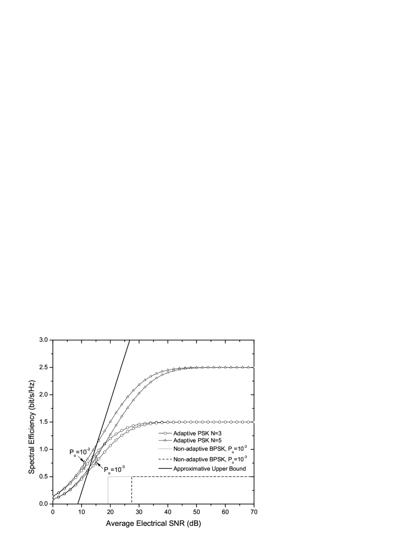
Figure 3: Spectral efficiency of the adaptive subcarrier PSK scheme when $\sigma_{x}=0.5$.

Figure 4: Average BER of the adaptive subcarrier PSK scheme when $\sigma_{x}=0.1$.

Figure 5: Average BER of the adaptive subcarrier PSK scheme when $\sigma_{x}=0.3$.

Figure 6: Average BER of the adaptive subcarrier PSK scheme when $\sigma_{x}=0.5$.

Figure 7: Spectral efficiency of the adaptive subcarrier PSK scheme for various MIMO configurations, when $N=5$, $P_{o}=10^{-3}$ and $\sigma_{x}=0.3$.

References

- [1] L. Andrews, R. L. Philips, and C. Y. Hopen, Laser Beam Scintillation with Applications. SPIE Press, 2001.
- [2] D. Kedar and S. Arnon, “Urban optical wireless communications networks: The main challenges and possible solutions,” IEEE Communications Magazine, vol. 42, no. 5, pp. 2–7, Feb. 2003.
- [3] V. W. S. Chan, “Free-Space Optical Communications,” Journal of Lightwave Technology, vol. 24, no. 12, pp. 4750–4762, Dec. 2006.
- [4] S. Karp, R. Gagliardi, S. E. Moran, and L. B. Stotts, Optical Channels. New York: Plenum, 1988.
- [5] X. Zhu and J. M. Kahn, “Performance bounds for coded free-space optical communications through atmospheric turbulence channels,” IEEE Trans. on Commun., vol. 51, no. 8, pp. 1233–1239, Aug. 2003.
- [6] M. Uysal, S. M. Navidpour, and J. Li, “Error rate performance of coded Free-Space optical links over strong turbulence channels,” IEEE Communications Letters, vol. 8, no. 10, pp. 635–637, Oct. 2004.
- [7] X. Zhu and J. M. Kahn, “Free-space optical communication through atmospheric turbulence channels,” IEEE Trans. Commun., vol. 50, no. 8, pp. 1293–1300, Aug. 2002.
- [8] M. L. B. Riediger, R. Schober, and L. Lampe, “Fast Multiple-Symbol Detection for free-space optical communications,” IEEE Trans. on Commun., vol. 57, no. 4, pp. 1119–1128, Apr. 2009.
- [9] ——, “Reduced-complexity multiple-symbol detection for free-space optical communications,” in GLOBECOM, Washington DC, USA, 2007, pp. 4548–4553.
- [10] ——, “Blind detection of on-off keying for free-space optical communications,” in VCCECE/CCGEI, Niagara Falls, Canada, 2008, pp. 1361–1364.
- [11] S. M. Navidpour and M. Uysal, “BER performance of free-space optical transmission with spatial diversity,” IEEE Trans. Wireless Commun., vol. 6, no. 8, pp. 2813–2819, Aug. 2007.
- [12] T. A. Tsiftsis, H. G. Sandalidis, G. K. Karagiannidis, and M. Uysal, “Optical wireless links with spatial diversity over strong atmospheric turbulence channels,” IEEE in Trans. on Wireless Communications, vol. 8, no. 2, pp. 951–957, Feb. 2009.
- [13] M. S. Alouini and A. J. Goldsmith, “Adaptive moulation over Nakagami fading channels,” Wireless Personal Communications, vol. 13, no. 1-2, pp. 119–143, May 2000.
- [14] B. K. Levitt, “Variable rate optical communication through the turbulent atmosphere,” Technical Report 483, Massachusetts Institute of Technology, Research Laboratory of Electronics, Aug. 1971. [Online]. Available: http://hdl.handle.net/1721.1/4260
- [15] J. Li and M. Uysal, “Achievable information rate for outdoor free space optical communication with intensity modulation and direct detection,” in Proc. of IEEE Global Communications Conference (GLOBECOM), San Francisco, CA, Nov. 2003, pp. 827–831.
- [16] M. Gubergrits, R. Goot, U. Mahlab, and S. Arnon, “Adaptive power control for satellite to ground laser communication,” International Journal of Satellite Communications and Networks, vol. 25, no. 4, pp. 323–348, Aug. 2007.
- [17] I. B. Djordjevic and G. T. Djordjevic, “On the communication over strong atmospheric turbulence channels by adaptive modulation and coding,” Optics Express, vol. 17, no. 20, pp. 18 250–18 262, 2009.
- [18] Q. Lu, Q. Liu, and G. S. Mitchell, “Performance analysis for optical wireless communication systems using sub-carrier psk intensity modulation through turbulent atmospheric channel,” in in Proc. IEEE Global Telecommun. Conf., Dallas, TX, USA, 2004, p. 1872 1875.
- [19] Q. Liu and Q. Li, “Subcarrier psk intensity modulation for optical wireless communications through turbulent atmospheric channel,” in Proc. IEEE Int. Conf. Commun, Seoul, Korea, 2005, p. 1761 1765.
- [20] J. Li, J. Q. Liu, and D. P. Taylor, “Optical communication using subcarrier PSK intensity modulation through atmospheric turbulence channels,” IEEE Trans. on Commun., vol. 55, no. 8, pp. 1598–1606, 2007.
- [21] S. Arnon, “Minimization of outage probability of WiMAX link supported by laser link between a high-altitude platform and a satellite,” Journal of Optical Society of America A, vol. 26, no. 7, pp. 1545–1552, Jul. 2009.
- [22] N. Cvijetic and T. Wang, “WiMAX over Free-Space Optics - Evaluating OFDM Multi-Subcarrier Modulation in Optical Wireless Channels,” in Sarnoff Symposium, 2006 IEEE, Mar. 2006, pp. 1–4.
- [23] G. Katz, S. Arnon, P. Goldgeier, Y. Hauptman, and N. Atias, “Cellular over optical wireless networks,” IEE Proc. Optoelectronics, vol. 153, no. 4, pp. 195–198, Aug. 2006.
- [24] R. You and J. M. Kahn, “Upper-Bounding the capacity of optical IM/DD channels with multiple-subcarrier modulation and fixed bias using trigonometric moment space method,” IEEE trans. on Information Theory, vol. 48, no. 2, pp. 514–523, Feb. 2002.
- [25] D. J. T. Heatley, D. R. Wisely, I. Neild, and P. Cochrane, “Optical wireless: the story so far,” IEEE Commun. Mag., vol. 36, no. 2, pp. 72–74, Dec. 1998.
- [26] E. Lee and V. Chan, “Part 1: Optical communication over the clear turbulent atmospheric channel using diversity,” IEEE Journal on Selected Areas in Commun., vol. 22, no. 9, pp. 71 896–1906, Nov. 2004.
- [27] J. G. Proakis, Digital Communications, 4th ed. New York: Mc Graw Hill, 2000.
- [28] M. Safari and M. Uysal, “Do we really need space-time coding for free-space optical communication with direct detection?” IEEE Transactions on Wireless Communications, vol. 7, no. 11, pp. 4445–4448, Nov. 2008.
- [29] I. S. Gradshteyn and I. M. Ryzhik, Table of Integrals, Series, and Products, 7th ed. New York: Academic, 2007.