New constraints on a light CP-odd Higgs boson and related NMSSM Ideal Higgs Scenarios.

Abstract:

Recent BaBar limits on $BR(\Upsilon(3S)\rightarrow\gamma a\rightarrow\gamma\tau^{+}\tau^{-})$ and $BR(\Upsilon(3S)\rightarrow\gamma a\rightarrow\gamma\mu^{+}\mu^{-})$ provide increased constraints on the $ab\overline{b}$ coupling of a CP-odd Higgs boson, $a$, with $m_{a}<M_{\Upsilon(3S)}$. We extract these limits from the BaBar data and compare to the limits previously obtained using other data sets, especially the CLEO-III $BR(\Upsilon(1S)\rightarrow\gamma\rightarrow\tau^{+}\tau^{-})$ limits. Comparisons are made to predictions in the context of “ideal”-Higgs NMSSM scenarios, in which the lightest CP-even Higgs boson, $h_{1}$, can have mass below $105~{}{\rm GeV}$ (as preferred by precision electroweak data) and yet can escape old LEP limits by virtue of decays to a pair of the lightest CP-odd Higgs bosons, $h_{1}\rightarrow a_{1}a_{1}$, with $m_{a_{1}}<2m_{B}$. Most such scenarios with $m_{a_{1}}<2m_{\tau}$ are eliminated, but the bulk of the $m_{a_{1}}>7.5~{}{\rm GeV}$ scenarios, which are theoretically the most favored, survive. We also outline the impact of the new ALEPH LEP results in the $e^{+}e^{-}\rightarrow Z+4\tau$ channel. For $\tan\beta\geq 3$, only NMSSM ideal Higgs scenarios with $m_{h_{1}}\mathrel{\raise 1.29167pt\hbox{$>$\kern-7.5pt\lower 4.30554pt\hbox{$\sim$}}}98~{}{\rm GeV}$ and $m_{a_{1}}$ close to $2m_{B}$ satisfy the ALEPH limits. For $\tan\beta\mathrel{\raise 1.29167pt\hbox{$<$\kern-7.5pt\lower 4.30554pt\hbox{$\sim$}}}2$, the ALEPH limits are easily satisfied for the most theoretically preferred NMSSM scenarios, which are those with $m_{a_{1}}$ close to $2m_{B}$ and $m_{h_{1}}\sim 90~{}{\rm GeV}-100~{}{\rm GeV}$.

1 Introduction

Many motivations for the existence of a light CP-odd $a$ Higgs boson have emerged in a variety of contexts in recent years. Of particular interest is the $m_{a}<2m_{B}$ region, for which a light Higgs, $h$, with SM-like $WW$, $ZZ$ and fermionic couplings can have mass $m_{h}\sim 100~{}{\rm GeV}$ while still being consistent with published LEP data by virtue of $h\rightarrow aa\rightarrow 4\tau$ or $4~{}jet$ decays being dominant [1, 2, 3, 4] (see also [5, 6]). Such a light Higgs provides perfect agreement with the rather compelling precision electroweak constraints, and for $BR(h\rightarrow aa)\mathrel{\raise 1.29167pt\hbox{$>$\kern-7.5pt\lower 4.30554pt\hbox{$\sim$}}}0.75$ also provides an explanation for the $\sim 2.3\sigma$ excess observed at LEP in $e^{+}e^{-}\rightarrow Zb\overline{b}$ in the region $M_{b\overline{b}}\sim 100~{}{\rm GeV}$. This is sometimes referred to as the “ideal” Higgs scenario. More generally, superstring modeling suggests the possibility of many light $a$’s. In this note, we update the analysis of [7] (see also [8]), quantifying the increased constraints on a general CP-odd $a$ arising from recent BaBar limits on the branching ratio for $\Upsilon(3S)\rightarrow\gamma a\rightarrow\gamma\tau^{+}\tau^{-}$ decays [9] and $\Upsilon(3S)\rightarrow\gamma a\rightarrow\gamma\mu^{+}\mu^{-}$ decays [10]. We also quantify the impact of these constraints, as well as the impact of the new ALEPH LEP results in the $e^{+}e^{-}\rightarrow Z+4\tau$ final state [11], on the Next-to-Minimal Supersymmetric Model (NMSSM) ideal Higgs scenarios.

The possibilities for discovery of an $a$ and limits on the $a$ are phrased in terms of the $a\mu^{-}\mu^{+}$, $a\tau^{-}\tau^{+}$, $ab\overline{b}$ and $at\overline{t}$ couplings defined via

$${\cal L}_{af\overline{f}}\equiv iC_{af\overline{f}}{ig_{2}m_{f}\over 2m_{W}}\overline{f}\gamma_{5}fa\,.$$ (1)

(Note: when discussing a generic CP-even (CP-odd) Higgs boson, we will use the notation $h$ ($a$). When specializing to the NMSSM context, we will use $h_{1},h_{2},h_{3}$ ($a_{1},a_{2}$) for the mass ordered Higgs states.) In this paper, we assume a Higgs model in which $C_{a\mu^{-}\mu^{+}}=C_{a\tau^{-}\tau^{+}}=C_{ab\overline{b}}$, as typified by a two-Higgs-doublet model (2HDM) of either type-I or type-II, or more generally if the lepton and down-type quark masses are generated by the same combination of Higgs fields. However, one should keep in mind that there are models in which $r=(C_{a\mu^{-}\mu^{+}}=C_{a\tau^{-}\tau^{+}})/C_{ab\overline{b}}\gg 1$ — such models include those in which the muon and tau masses are generated by different Higgs fields than the $b$ mass. In a 2HDM of type-II and in the MSSM, $C_{a\mu^{-}\mu^{+}}=C_{a\tau^{-}\tau^{+}}=C_{ab\overline{b}}=\tan\beta$ (where $\tan\beta=h_{u}/h_{d}$ is the ratio of the vacuum expectation values for the doublets giving mass to up-type quarks vs. down-type quarks) and $C_{at\overline{t}}=\cot\beta$. These results are modified in the NMSSM (see, e.g. [12] and [13]). In the NMSSM, both $C_{a_{1}t\overline{t}}$ and $C_{a_{1}b\overline{b}}=C_{a_{1}\mu^{-}\mu^{+}}=C_{a_{1}\tau^{-}\tau^{+}}$ are multiplied by a factor $\cos\theta_{A}$, where $\cos\theta_{A}$ is defined by

$$a_{1}=\cos\theta_{A}a_{MSSM}+\sin\theta_{A}a_{S},$$ (2)

where $a_{1}$ is the lightest of the 2 CP-odd scalars in the model. Above, $a_{MSSM}$ is the CP-odd (doublet) scalar in the MSSM sector of the NMSSM and $a_{S}$ is the additional CP-odd singlet scalar of the NMSSM. In terms of $\cos\theta_{A}$, $C_{a_{1}\mu^{-}\mu^{+}}=C_{a_{1}\tau^{-}\tau^{+}}=C_{a_{1}b\overline{b}}=\cos\theta_{A}\tan\beta$ and $C_{a_{1}t\overline{t}}=\cos\theta_{A}\cot\beta$. Quite small values of $\cos\theta_{A}$ are natural when $m_{a_{1}}$ is small as a result of being close to the $U(1)_{R}$ limit of the model. In the most general Higgs model, $C_{a\mu^{-}\mu^{+}}$, $C_{a\tau^{-}\tau^{+}}$, $C_{ab\overline{b}}$ and $C_{at\overline{t}}$ will be more complicated functions of the vevs of the Higgs fields and the structure of the Yukawa couplings. In this paper, we assume $C_{a\mu^{-}\mu^{+}}=C_{a\tau^{-}\tau^{+}}=C_{ab\overline{b}}$ and $C_{ab\overline{b}}/C_{at\overline{t}}=\tan^{2}\beta$.

For the analysis presented in this paper, we neglect the possible presence of large corrections at large $\tan\beta$ to $C_{ab\overline{b}}$ from SUSY loops [16, 17, 18]. These are typically characterized by the quantity $\Delta_{b}$ which is crudely of order ${\mu\tan\beta\over 16\pi^{2}M_{SUSY}}$. The correction to the coupling takes the form of $1/(1+\Delta_{b})$. Since $\mu$ can have either sign, $C_{ab\overline{b}}$ can be either enhanced or suppressed relative to equality with $C_{a\tau^{-}\tau^{+}}$ (the corrections to which are much smaller) and $C_{a\mu^{-}\mu^{+}}$ (the corrections to which are negligible). This same correction factor would apply to $C_{a_{1}b\overline{b}}$ in the NMSSM case.

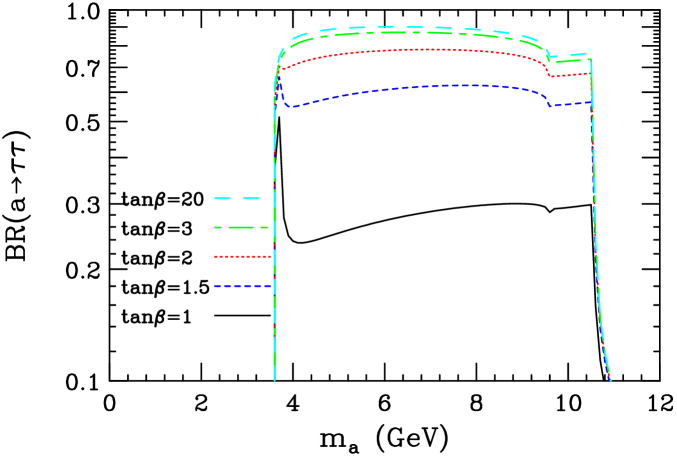
Figure 1: $BR(a\rightarrow\tau^{+}\tau^{-})$ is plotted as a function of $m_{a}$ for a variety of $\tan\beta$ values. $BR(a\rightarrow\tau^{+}\tau^{-})$ is independent of $\cos\theta_{A}$.

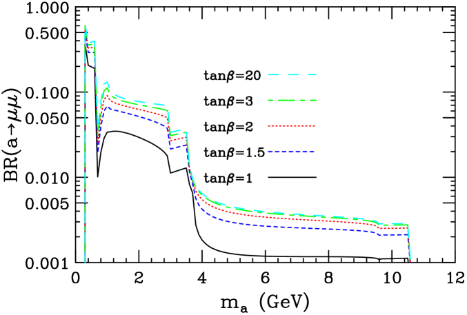
Figure 2: $BR(a\rightarrow\mu^{+}\mu^{-})$ is plotted as a function of $m_{a}$ for a variety of $\tan\beta$ values. $BR(a\rightarrow\mu^{+}\mu^{-})$ is independent of $\cos\theta_{A}$.

Key ingredients in understanding current limits are the branching ratios for $a\rightarrow\tau^{+}\tau^{-}$ and $a\rightarrow\mu^{+}\mu^{-}$ decays. These branching ratios are plotted in Figs. 1 and 2. (It is important to note that at tree-level the $a$ branching ratios apply equally to the $a_{1}$, independent of $\cos\theta_{A}$, due to the absence of tree-level $a,a_{1}\rightarrow VV$ couplings and similar.) Note that $BR(a\rightarrow\tau^{+}\tau^{-})$ and $BR(a\rightarrow\mu^{+}\mu^{-})$ change very little with increasing $\tan\beta$ at any given $m_{a}$ once $\tan\beta\mathrel{\raise 1.29167pt\hbox{$>$\kern-7.5pt\lower 4.30554pt\hbox{$\sim$}}}2$. We note that in the region $m_{a}<2m_{\tau}$, $BR(a\rightarrow\mu^{+}\mu^{-})$ has some significant structures that arise from the fact that $BR(a\rightarrow gg)$ is substantial and varies rapidly in that region. The rapid variation in $BR(a\rightarrow gg)$ occurs when $m_{a}$ crosses the internal quark loop thresholds. At higher $m_{a}$, $BR(a\rightarrow gg)$ becomes significant for $m_{a}$ near $2m_{b}$. We plot $BR(a\rightarrow gg)$ in Fig. 3. Note that in the calculation of $BR(a\rightarrow gg)$ we have chosen to keep the loop quark masses equal to the current quark masses in our calculations, whereas we employ thresholds of $2m_{K}$ and $2m_{D}$ for the strange quark and charm quark final states, respectively. Some changes in the structures present, especially in $BR(a\rightarrow\mu^{+}\mu^{-})$, take place if, instead, the loop quark masses are set equal to the true physical threshold masses.

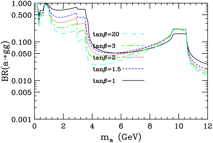
Figure 3: $BR(a\rightarrow gg)$ is plotted as a function of $m_{a}$ for a variety of $\tan\beta$ values.

Of course, the above branching ratios are impacted by the $a\rightarrow c\overline{c}$ and $a\rightarrow s\overline{s}$ channels, the latter being a rather important competitor for smaller $\tan\beta$ and $m_{a}>2m_{K}$. Plots of these branching ratios appear in Figs. 4 and 5, respectively.

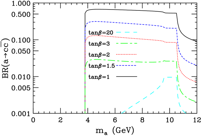
Figure 4: $BR(a\rightarrow c\overline{c})$ is plotted as a function of $m_{a}$ for a variety of $\tan\beta$ values.

Figure 5: $BR(a\rightarrow s\overline{s})$ is plotted as a function of $m_{a}$ for a variety of $\tan\beta$ values.

It is relevant to note that both $BR(a\rightarrow\mu^{+}\mu^{-})$ and $BR(a\rightarrow\tau^{+}\tau^{-})$ tend to decline slowly as $m_{a}$ is increased, with a significant dip in the latter for $m_{a}$ close to $2m_{b}$ where the $b$-loop contribution to the $gga$ coupling is close to the point at which the internal $b$’s can go on-shell . This has important implications for using these channels to probe the $9~{}{\rm GeV}\mathrel{\raise 1.29167pt\hbox{$<$\kern-7.5pt\lower 4.30554pt\hbox{$\sim$}}}m_{a}\mathrel{\raise 1.29167pt\hbox{$<$\kern-7.5pt\lower 4.30554pt\hbox{$\sim$}}}2m_{B}$ region in which many parameter choices lead to absence of light-$a_{1}$ finetuning in the NMSSM. “Light-$a_{1}$” finetuning is characterized numerically by a quantity we call $G$, defined in [3], that gives the degree of precision with which the $A_{\lambda}$ and $A_{\kappa}$ soft-SUSY-breaking NMSSM parameters must be chosen in order that $m_{a_{1}}<2m_{B}$ and $BR(h_{1}\rightarrow a_{1}a_{1})>0.75$ as required to allow $m_{h_{1}}\mathrel{\raise 1.29167pt\hbox{$<$\kern-7.5pt\lower 4.30554pt\hbox{$\sim$}}}105~{}{\rm GeV}$ to be consistent with published LEP constraints when the $h_{1}$ has SM-like $h_{1}ZZ$ coupling. Absence of light-$a_{1}$ finetuning is equivalent to $G\mathrel{\raise 1.29167pt\hbox{$<$\kern-7.5pt\lower 4.30554pt\hbox{$\sim$}}}20$. Typically, this condition is satisfied only when the light $a_{1}$ of the NMSSM is mainly singlet. For example, at $\tan\beta=10$, $0.6\mathrel{\raise 1.29167pt\hbox{$<$\kern-7.5pt\lower 4.30554pt\hbox{$\sim$}}}|C_{a_{1}b\overline{b}}|\mathrel{\raise 1.29167pt\hbox{$<$\kern-7.5pt\lower 4.30554pt\hbox{$\sim$}}}1.2$ ($0.06\mathrel{\raise 1.29167pt\hbox{$<$\kern-7.5pt\lower 4.30554pt\hbox{$\sim$}}}|\cos\theta_{A}|\mathrel{\raise 1.29167pt\hbox{$<$\kern-7.5pt\lower 4.30554pt\hbox{$\sim$}}}0.12$) is required if $G<20$ is imposed as well as requiring $m_{a_{1}}<2m_{B}$ and $BR(h_{1}\rightarrow a_{1}a_{1})>0.75$, with $G<10$ achieved only for $\cos\theta_{A}\in[-0.08,-0.1]$, corresponding to $|C_{a_{1}b\overline{b}}|\in[0.8,1]$. The $G<10$ range for $\tan\beta=3$ is broader, $\cos\theta_{A}\in[-0.28,-0.08]$, while that for $\tan\beta=50$ is narrow, $\cos\theta_{A}\in[-0.04,-0.06]$, yielding $|C_{a_{1}b\overline{b}}|\in[0.24,0.84]$ and $|C_{a_{1}b\overline{b}}|\in[2,3]$, respectively. Thus, lower $\tan\beta$ values will be harder to probe using direct limits on the $a_{1}$.

We emphasize that, given the importance of the exact $a$ or $a_{1}$ branching ratios in the analyses that follow, additional attention to the most precise predictions possible is warranted. Our $a,a_{1}$ decay results employ a branching ratio program that is taken from HDECAY [19]. We note that the $a_{1}$ branching ratios obtained using this program are somewhat different than those that one obtains using the $a_{1}$ decay formulae in the current version of NMHDECAY. In particular, the former often predicts smaller $BR(a_{1}\rightarrow\tau^{+}\tau^{-})$ than does the latter.

2 Upsilon decay limits compared to NMSSM predictions

Figure 6: $BR(\Upsilon(3S)\rightarrow\gamma a_{1})\times BR(a_{1}\rightarrow\tau^{+}\tau^{-})$ for NMSSM scenarios with various ranges for $m_{a_{1}}$: medium grey (red) = $2m_{\tau}<m_{a_{1}}<7.5~{}{\rm GeV}$; light grey (green) = $7.5~{}{\rm GeV}<m_{a_{1}}<8.8~{}{\rm GeV}$; and black = $8.8~{}{\rm GeV}<m_{a_{1}}<2m_{B}~{}{\rm GeV}$. The plots are for $\tan\beta=3,10,50$, respectively. The left-hand window in each plot shows results for a “fixed-$\mu$-scan” as defined in the text (and in Ref. [20]) The right-hand window shows results for $F<15$ points found using a “full scan” as defined in the text.

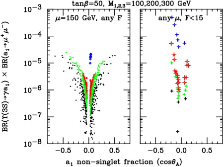
Figure 7: We plot $BR(\Upsilon(3S)\rightarrow\gamma a_{1})\times BR(a_{1}\rightarrow\mu^{+}\mu^{-})$ using the same notation and scanning procedures as described in the caption of Fig. 6.

Before continuing with the general analysis, it is useful to compare the limits of [9] and [10] with the predictions of the NMSSM. This comparison is done for the same two types of scans as in the earlier paper [20], except that here we focus on the $3S$ state rather than the $1S$ state. In both scans, we hold the gaugino soft-SUSY-breaking parameters of the NMSSM fixed at $M_{1,2,3}(m_{Z})=100,200,300~{}{\rm GeV}$ and fix $\tan\beta$. In the first type of scan, called a “fixed-$\mu$ scan”, we scan over the NMSSM soft-SUSY-breaking Higgs potential parameters $A_{\lambda}$ and $A_{\kappa}$ keeping the effective $\mu$ parameter of the model fixed at the representative value of $\mu=150~{}{\rm GeV}$ (at $\tan\beta=10$ and $50$) or $\mu=152~{}{\rm GeV}$ (at $\tan\beta=3$ for which we must take $\mu=152~{}{\rm GeV}$ in order to get physically allowable scenarios). In addition, in the fixed-$\mu$ scans we have kept the scalar soft-SUSY-breaking masses fixed at common value of $M_{SUSY}=300~{}{\rm GeV}$ and the $A$ soft-SUSY-breaking parameters fixed to a common value of $-300~{}{\rm GeV}$. In the second type of scan, termed a “full scan”, we have allowed $\mu$ to vary and have also allowed the soft-SUSY-breaking scalar masses and $A$ parameters to vary (independently of one another). In the full scan results presented we have kept only scenarios with very low electroweak finetuning, as characterized by the parameter $F$ (see [1] for more details) being smaller than $15$, where $F<15$ corresponds to absence of electroweak finetuning. $F<15$ scenarios only arise for $m_{h_{1}}\mathrel{\raise 1.29167pt\hbox{$<$\kern-7.5pt\lower 4.30554pt\hbox{$\sim$}}}105~{}{\rm GeV}$ and are thus automatically “ideal” in the precision electroweak sense. As part of the fixed-$\mu$ scans and the full scans, we have required that the CP-even $h_{1}$ escape published LEP limits by virtue of dominant $h_{1}\rightarrow a_{1}a_{1}\rightarrow 4\tau$ or $4~{}jet$ decays. In the forthcoming plots, the left-hand windows correspond to fixed-$\mu$ scan results and the right-hand windows give the results of a full scan for the same $\tan\beta$ value.

Our results for the $\tau^{+}\tau^{-}$ final state are shown in Fig. 6 and those for the $\mu^{+}\mu^{-}$ final state are shown in Fig. 7. Let us focus first on the $\tau^{+}\tau^{-}$ final state. The 90% CL $BR(\Upsilon(3S)\rightarrow\gamma a)\times BR(a\rightarrow\tau^{+}\tau^{-})$ limits from BaBar range from $\sim 10^{-5}$ at $m_{a}$ just above $2m_{\tau}$ with a long plateau at the $3-7\times 10^{-5}$ until $m_{a}$ passes above $10~{}{\rm GeV}$ where the limit is of order $10^{-4}$. In Fig. 6, the black points have high $m_{a_{1}}$ ($8.8~{}{\rm GeV}<m_{a_{1}}\leq 2m_{B}$), the light grey (green) points have $7.5~{}{\rm GeV}<m_{a_{1}}\leq 8.8~{}{\rm GeV}$ and the medium grey (red) points have $2m_{\tau}<m_{a_{1}}\leq 7.5~{}{\rm GeV}$. Let us first discuss $\tan\beta=10$ results, since these can be compared to those for $\Upsilon(1S)\rightarrow\gamma a_{1}\rightarrow\gamma\tau^{+}\tau^{-}$ presented in Ref. [20]. From comparing the BaBar limits summarized above with the relevant plot of Fig. 6, we see that most of the $m_{a_{1}}<7.5~{}{\rm GeV}$ points are excluded, about half of the $7.5~{}{\rm GeV}<m_{a_{1}}\leq 8.8~{}{\rm GeV}$ are excluded, but that many fewer of the $m_{a_{1}}>8.8~{}{\rm GeV}$ points are excluded. Still, exclusions of this higher $m_{a_{1}}$ region are much superior to those from the CLEO-III $\Upsilon(1S)$ data [21], which excluded none of the black points, a small fraction of the green points and about half of the red points. This ability to probe to higher $m_{a_{1}}$ using the $\Upsilon(3S)$ is particularly relevant in the NMSSM context since the GUT-scale tunings of $A_{\lambda}$ and $A_{\kappa}$ needed to obtain $m_{a_{1}}<2m_{B}$ while at the same time having $BR(h_{1}\rightarrow a_{1}a_{1})\mathrel{\raise 1.29167pt\hbox{$>$\kern-7.5pt\lower 4.30554pt\hbox{$\sim$}}}0.7$, as required in the ideal Higgs scenario, is minimal for $m_{a_{1}}$ values close to $2m_{B}$. For $\tan\beta=50$, one finds that almost all the $2m_{\tau}<m_{a_{1}}<8.8~{}{\rm GeV}$ scenarios are excluded, but that lots of $m_{a_{1}}>8.8~{}{\rm GeV}$ points survive. In contrast, for $\tan\beta=3$ the BaBar results only significantly constrain the region $2m_{\tau}<m_{a_{1}}\leq 7.5~{}{\rm GeV}$.

We now turn to the $\mu^{+}\mu^{-}$ final state. The 90% CL $BR(\Upsilon(3S)\rightarrow\gamma a)\times BR(a\rightarrow\mu^{+}\mu^{-})$ limits from BaBar are $\sim 1-3.5\times 10^{-6}$ for $m_{a}\mathrel{\raise 1.29167pt\hbox{$<$\kern-7.5pt\lower 4.30554pt\hbox{$\sim$}}}1~{}{\rm GeV}$, $\sim 1-2\times 10^{-6}$ for $1\mathrel{\raise 1.29167pt\hbox{$<$\kern-7.5pt\lower 4.30554pt\hbox{$\sim$}}}m_{a}<2m_{\tau}$, $\sim 1-3\times 10^{-6}$ for $2m_{\tau}\mathrel{\raise 1.29167pt\hbox{$<$\kern-7.5pt\lower 4.30554pt\hbox{$\sim$}}}m_{a}\mathrel{\raise 1.29167pt\hbox{$<$\kern-7.5pt\lower 4.30554pt\hbox{$\sim$}}}7.5~{}{\rm GeV}$, and $\sim 1-5\times 10^{-6}$ for $7.5~{}{\rm GeV}\mathrel{\raise 1.29167pt\hbox{$<$\kern-7.5pt\lower 4.30554pt\hbox{$\sim$}}}m_{a_{1}}\mathrel{\raise 1.29167pt\hbox{$<$\kern-7.5pt\lower 4.30554pt\hbox{$\sim$}}}9.2~{}{\rm GeV}$. In Fig. 7 the black points have high $m_{a_{1}}$ ($8.8~{}{\rm GeV}<m_{a_{1}}\leq 2m_{B}$), the light grey (green) points have $7.5~{}{\rm GeV}<m_{a_{1}}\leq 8.8~{}{\rm GeV}$, the medium grey (red) points have $2m_{\tau}<m_{a_{1}}\leq 7.5~{}{\rm GeV}$ and the darker grey (blue) points have $m_{a_{1}}<2m_{\tau}$. At $\tan\beta=3$, the $\mu^{+}\mu^{-}$ final state data eliminates more than 4/5 of the NMSSM model points in the $m_{a_{1}}<2m_{\tau}$ mass range, but only a small number of the NMSSM points for $2m_{\tau}<m_{a_{1}}<7.5~{}{\rm GeV}$ and none of the points with $7.5~{}{\rm GeV}\mathrel{\raise 1.29167pt\hbox{$<$\kern-7.5pt\lower 4.30554pt\hbox{$\sim$}}}m_{a_{1}}$. At $\tan\beta=10$, all $m_{a_{1}}<2m_{\tau}$ NMSSM points are eliminated by the $\mu^{+}\mu^{-}$ data as well as a small fraction of the $2m_{\tau}<m_{a_{1}}<7.5~{}{\rm GeV}$ and $7.5~{}{\rm GeV}<m_{a_{1}}<8.8~{}{\rm GeV}$ points, but none of the $8.8~{}{\rm GeV}<m_{a_{1}}$ points. At $\tan\beta=50$, all $m_{a_{1}}<2m_{\tau}$ NMSSM points are again eliminated, perhaps half of the $2m_{\tau}<m_{a_{1}}<7.5~{}{\rm GeV}$ points are eliminated, a still significant fraction of the $7.5~{}{\rm GeV}<m_{a_{1}}<8.8~{}{\rm GeV}$ points are eliminated, and even a significant number of the $8.8~{}{\rm GeV}<m_{a_{1}}$ points are eliminated.

To summarize, only the $\mu^{+}\mu^{-}$ channel provides constraints for $m_{a_{1}}<2m_{\tau}$ and almost all the ideal-Higgs-like NMSSM scenarios with $\tan\beta\geq 3$ are eliminated. For $2m_{\tau}<m_{a_{1}}$, the $\tau^{+}\tau^{-}$ channel provides the most eliminations for all $\tan\beta$. Certainly, the BaBar $\Upsilon(3S)$ results are a big stride relative to the CLEO-III $\Upsilon(1S)$ results, especially at $m_{a_{1}}<2m_{\tau}$ and at high $m_{a_{1}}$. Of course, it is important to note that the NMSSM scenarios most favored in order to minimize light-$a_{1}$ finetuning have $m_{a_{1}}$ very near $2m_{B}$ and thus cannot be limited by Upsilon decays.

3 General limits on the $ab\overline{b}$ coupling

Our ultimate goal is to use the $\Upsilon_{3S}$ limits in combination with other available limits to extract limits on $|C_{ab\overline{b}}|$. The older experiments that provide the most useful constraints are as follows. Prior to the recent BaBar data, for $2m_{\tau}<m_{a}<9.2~{}{\rm GeV}$ the recent CLEO-III [21] limits on $\Upsilon(1S)\rightarrow\gamma a\rightarrow\gamma\tau^{+}\tau^{-}$ were the strongest. For $9.2~{}{\rm GeV}<m_{a}<M_{\Upsilon(1S)}$, mixing of the $a$ with various $\eta_{b}$ and $\chi_{0}$ bound states becomes crucial [22]. Ref. [21] gives results for $C_{ab\overline{b}}^{\rm max}$ in this $m_{a}$ range without taking this mixing into account but notes that their limits cannot be relied upon for $m_{a}>9.2~{}{\rm GeV}$. Whether additional limits can be extracted from lepton non-universality studies in the $9.2<m_{a}<M_{\Upsilon(1S)}$ region is being studied [23]. OPAL limits [24] (which assume $BR(a\rightarrow\tau^{+}\tau^{-})=1$) on $e^{+}e^{-}\rightarrow b\overline{b}\tau^{+}\tau^{-}$ become numerically relevant for roughly $9~{}{\rm GeV}<m_{a}<2m_{B}$. Ref. [24] converts these limits to limits on the $ab\overline{b}$ coupling using the modeling of [22]. These are the only LEP limits in the $M_{\Upsilon(3S)}<m_{a}<2m_{B}$ range and continue to be relevant up to $12~{}{\rm GeV}$. Above $m_{a}=2m_{B}$ these $ab\overline{b}$ coupling limits become quite weak due to the $\eta_{b}-a$ mixing uncertainties and the decrease of $BR(a\rightarrow\tau^{+}\tau^{-})$. For $m_{a}\geq 12~{}{\rm GeV}$, limits on the $ab\overline{b}$ coupling can be extracted from $e^{+}e^{-}\rightarrow b\overline{b}a\rightarrow b\overline{b}b\overline{b}$ [25]. One should also keep in mind that values of $|C_{ab\overline{b}}|$ above 50 raise issues of non-perturbativity of the $ab\overline{b}$ coupling and are likely to be in conflict with Tevatron limits on $b\overline{b}a$ production [26]. The limits, $C_{ab\overline{b}}^{\rm max}$, on $C_{ab\overline{b}}$ coming from all data, including the recent BaBar results, are plotted in Fig. 8 for various $R_{b/t}\equiv\sqrt{C_{ab\overline{b}}/C_{at\overline{t}}}$ values. (In a 2HDM model type-II context, $R_{b/t}=\tan\beta$.) Note the rapid deterioration as $m_{a}\rightarrow M_{\Upsilon(3S)}$. The variation with $R_{b/t}$ arises because $BR(a\rightarrow\tau^{+}\tau^{-})$ varies with $R_{b/t}$ as shown in Fig. 1. Basically, for $\tan\beta>1$ the BaBar results provide the most stringent limits. For $\tan\beta=0.5$ the $a$ decays to a complicated mix of channels and the old CUSB-II limits (which were independent of the exact $a$ final state) are strongest for $m_{a}\mathrel{\raise 1.29167pt\hbox{$<$\kern-7.5pt\lower 4.30554pt\hbox{$\sim$}}}8~{}{\rm GeV}$.

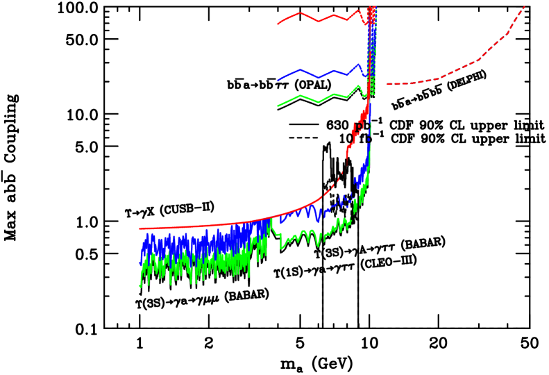
Figure 8: Upper limit, $C_{ab\overline{b}}^{\rm max}$, on $|C_{ab\overline{b}}|$ as a function of $m_{a}$ for a variety of $\tan\beta$ values coming directly from experimental data. The highest (red) curve is for $\tan\beta=0.5$, the other curves, in order of decreasing $C_{ab\overline{b}}^{\rm max}$ are for $\tan\beta=1$, $\tan\beta=2$ and $\tan\beta\geq 3$.

In Fig. 8, we have also plotted limits extracted [27] from Tevatron data using a reinterpretation of a CDF analysis performed over the range $6.3~{}{\rm GeV}\leq M_{\mu^{+}\mu^{-}}\leq 9~{}{\rm GeV}$ [28, 29]. This analysis placed limits on the ratio $R={\sigma(\epsilon)BR(\epsilon\rightarrow\mu^{+}\mu^{-})\over\sigma(\Upsilon_{1S})BR(\Upsilon_{1S}\rightarrow\mu^{+}\mu^{-})}$, where $\epsilon$ was a narrow resonance produced in the same manner as the $\Upsilon_{1S}$. Fluctuations of $R$ above a smooth fit to the overall spectrum were searched for and 90% CL limits were placed on $R$. It is relatively straightforward to apply this analysis to place limits on $R={\sigma(a)BR(a\rightarrow\mu^{+}\mu^{-})\over\sigma(\Upsilon_{1S})BR(\Upsilon_{1S}\rightarrow\mu^{+}\mu^{-})}$. The 90% CL limits on $R$ corresponding to the available $L=630~{}\mbox{pb}^{-1}$ data set are then easily converted to limits on $|C_{ab\overline{b}}|$. These limits as a function of $m_{a}$ are those plotted as the solid histogram. A simple statistical extrapolation of these limits to $L=10~{}{\mbox{fb}^{-1}}$ (an integrated luminosity that will soon be available) is shown as the dashed histogram. These limits hold for $\tan\beta>2$. We see that these limits improve rapidly as $m_{a}$ increases. While the $L=630~{}\mbox{pb}^{-1}$ limits are not quite competitive with the limits from BaBar data at $m_{a}\sim 9~{}{\rm GeV}$, we observe that the $L=10~{}{\mbox{fb}^{-1}}$ limits will actually be slightly better if the extrapolation holds.

While $\Upsilon(nS)$-based limits are kinematically limited and become weak for $m_{a}\mathrel{\raise 1.29167pt\hbox{$>$\kern-7.5pt\lower 4.30554pt\hbox{$\sim$}}}9.6~{}{\rm GeV}$, there is no such kinematic limitation for limits based on hadronic collider data. In fact, CDF measured the $M_{\mu^{+}\mu^{-}}$ spectrum above $9~{}{\rm GeV}$, but did not perform the easily reinterpreted $R$ analysis in the region $M_{\mu^{+}\mu^{-}}>9~{}{\rm GeV}$. In [27], we estimated the 90% CL limits from the $L=630~{}\mbox{pb}^{-1}$ measurements in the $M_{\mu^{+}\mu^{-}}>9~{}{\rm GeV}$ region (out to $M_{\mu^{+}\mu^{-}}=12~{}{\rm GeV}$) and found that, in the range $9.6~{}{\rm GeV}\mathrel{\raise 1.29167pt\hbox{$<$\kern-7.5pt\lower 4.30554pt\hbox{$\sim$}}}m_{a}\mathrel{\raise 1.29167pt\hbox{$<$\kern-7.5pt\lower 4.30554pt\hbox{$\sim$}}}2m_{B}$, implied limits on $|C_{ab\overline{b}}|$ were of order $|C_{ab\overline{b}}|<1.6-1.8$ for $m_{a}$ outside the $\Upsilon_{2S}$ and $\Upsilon_{3S}$ peaks. At both peaks we found $|C_{ab\overline{b}}|\mathrel{\raise 1.29167pt\hbox{$<$\kern-7.5pt\lower 4.30554pt\hbox{$\sim$}}}2$. For $L=10~{}{\mbox{fb}^{-1}}$, these limits should come down to $|C_{ab\overline{b}}|\mathrel{\raise 1.29167pt\hbox{$<$\kern-7.5pt\lower 4.30554pt\hbox{$\sim$}}}1$, and begin to constrain the most preferred NMSSM parameter regions, especially for large $\tan\beta$.

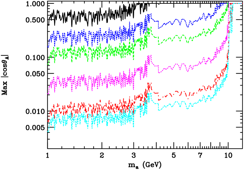
Figure 9: $\cos\theta_{A}^{\rm max}$ in the NMSSM (where $C_{ab\overline{b}}=\cos\theta_{A}\tan\beta$) as a function of $m_{a}$. The different curves correspond to $\tan\beta=1$ (upper curve), $1.7$, $3$, $10$, $32$ and $50$ (lowest curve). CDF/Tevatron constraints do not affect this plot.

4 Implications of general $ab\overline{b}$ limits for NMSSM scenarios

In the NMSSM, we note that it is always possible to choose $\cos\theta_{A}$ so that the limits on $C_{a_{1}b\overline{b}}$ as a function of $\tan\beta$ are satisfied. The maximum allowed value of $|\cos\theta_{A}|$, $\cos\theta_{A}^{\rm max}$, as a function of $m_{a}=m_{a_{1}}$ for various $\tan\beta$ values is plotted in Fig. 9. Constraints are strongest for $m_{a}\mathrel{\raise 1.29167pt\hbox{$<$\kern-7.5pt\lower 4.30554pt\hbox{$\sim$}}}9~{}{\rm GeV}$ for which Upsilon limits are relevant, and deteriorate rapidly above that. As seen in Fig. 8, currently the limits from the Tevatron/CDF data are not as strong as those from the BaBar $\Upsilon_{3S}$ data and do not affect this plot.

As an aside regarding the general 2HDM(II) model, we note that any point for which $\cos\theta_{A}^{\rm max}$ is smaller than $1$ corresponds to an $m_{a}$ and $\tan\beta$ choice that is not consistent with the experimental limits. Disallowed regions emerge in the range $m_{a}\mathrel{\raise 1.29167pt\hbox{$<$\kern-7.5pt\lower 4.30554pt\hbox{$\sim$}}}2m_{\tau}$ for $\tan\beta=1$, rising quickly to $m_{a}\mathrel{\raise 1.29167pt\hbox{$<$\kern-7.5pt\lower 4.30554pt\hbox{$\sim$}}}9~{}{\rm GeV}$ for $\tan\beta=1.7$ and $m_{a}\mathrel{\raise 1.29167pt\hbox{$<$\kern-7.5pt\lower 4.30554pt\hbox{$\sim$}}}10~{}{\rm GeV}$ for $\tan\beta\geq 3$. These excluded regions apply to any light doublet CP-odd Higgs boson, including the beyond the MSSM scenarios of [30, 31, 32] which are consistent with other experimental constraints for $\tan\beta\mathrel{\raise 1.29167pt\hbox{$<$\kern-7.5pt\lower 4.30554pt\hbox{$\sim$}}}2.5$.

We can illustrate the effects of the limits plotted in Fig. 9 on preferred NMSSM scenarios. Relevant plots appear below. The first set of plots, Figs. 10, 11 and 12, for $\tan\beta=3$, $10$, and $50$, respectively, show results for “fixed-$\mu$ scans” (see earlier definition). In each figure, the left-hand plot gives the light-$a_{1}$ finetuning measure $G$ as a function of $\cos\theta_{A}$ before imposing the $\cos\theta_{A}^{\rm max}$ constraint while the right-hand plot gives $G$ as a function of $\cos\theta_{A}$ after imposing $\cos\theta_{A}^{\rm max}$. The point notation is according to $m_{a_{1}}$: blue for $m_{a_{1}}<2m_{\tau}$, red for $2m_{\tau}<m_{a_{1}}<7.5~{}{\rm GeV}$, green for $7.5~{}{\rm GeV}<m_{a_{1}}<8.8~{}{\rm GeV}$ and black for $8.8~{}{\rm GeV}<m_{a_{1}}<2m_{B}$. We see that the bulk of points with $m_{a_{1}}<7.5~{}{\rm GeV}$ are eliminated by the $\cos\theta_{A}^{\rm max}$ limit and that the points with $m_{a_{1}}>7.5~{}{\rm GeV}$ at large $|\cos\theta_{A}|$ are also eliminated.

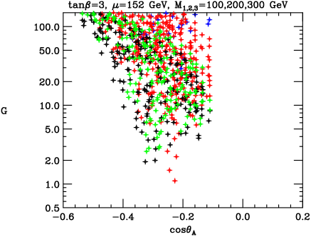
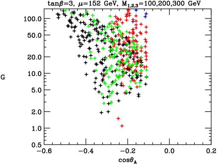
Figure 10: Light-$a_{1}$ finetuning measure $G$ before and after imposing limits $|\cos\theta_{A}|\leq\cos\theta_{A}^{\rm max}$. These plots are those obtained for “fixed-$\mu$ scans” with $\mu=152~{}{\rm GeV}$ and setting $\tan\beta=3$. Note that many points with low $m_{a_{1}}$ and large $|\cos\theta_{A}|$ are eliminated by the $|\cos\theta_{A}|<\cos\theta_{A}^{\rm max}$ requirement, including almost all the $m_{a_{1}}<2m_{\tau}$ (blue) points and a good fraction of the $2m_{\tau}<m_{a_{1}}<7.5~{}{\rm GeV}$ (red) points.

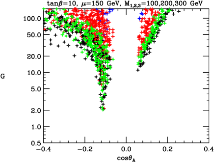
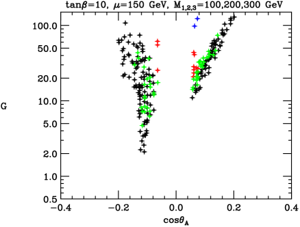
Figure 11: As in Fig. 10, but for $\mu=150~{}{\rm GeV}$ and $\tan\beta=10$. Note that many points with low $m_{a_{1}}$ and large $|\cos\theta_{A}|$ are eliminated, including almost all the $m_{a_{1}}<2m_{\tau}$ (blue) points and $2m_{\tau}<m_{a_{1}}<7.5~{}{\rm GeV}$ (red) points.

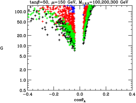
Figure 12: As in Fig. 10, but for $\mu=150~{}{\rm GeV}$ and $\tan\beta=50$. Note that the only surviving points are those with $m_{a_{1}}>8.8~{}{\rm GeV}$ (black points) at small $|\cos\theta_{A}|$.

The second set of plots below, Figs. 13, 14 and 15, show results for “full scans”, as defined previously, for $\tan\beta=3$, $10$, and $50$, respectively. Only points with electroweak finetuning measure $F$ below $15$ are plotted. As in the previous set of plots, the left-hand plot in each figure shows the points allowed without the $\cos\theta_{A}^{\rm max}$ constraint and the right-hand plot displays the points remaining after imposing $\cos\theta_{A}^{\rm max}$. The limited statistics for the parameter scans that search for points with low $F$ are apparent, but the trends are clearly the same as in the fixed $\mu$ scans presented previously.

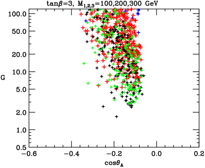
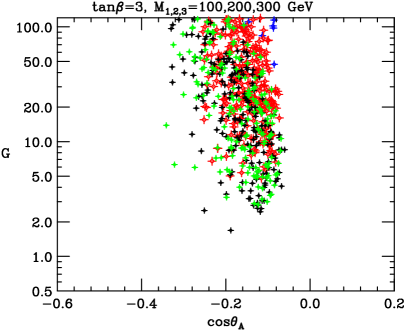
Figure 13: Light-$a_{1}$ finetuning measure $G$ before and after imposing $|\cos\theta_{A}|\leq\cos\theta_{A}^{\rm max}$. These are the results obtained using a “full scan” at $\tan\beta=3$. Only solutions with electroweak finetuning measure $F<15$ are retained. Note that a good fraction of the $m_{a_{1}}<2m_{\tau}$ (blue) points and $2m_{\tau}<m_{a_{1}}<7.5~{}{\rm GeV}$ (red) points are eliminated by the $\cos\theta_{A}^{\rm max}$ cut.

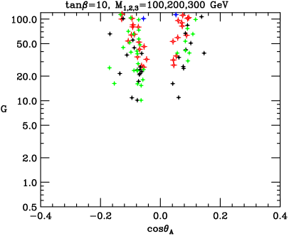
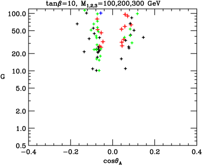
Figure 14: As in Fig. 13, but for $\tan\beta=10$. Note that many points with lower $m_{a_{1}}$ and large $|\cos\theta_{A}|$ are eliminated by the $|\cos\theta_{A}|\leq\cos\theta_{A}^{\rm max}$ cut.

Figure 15: As in Fig. 13, but for $\tan\beta=50$. Note that no $F<15$ points found in our scans survive the $|\cos\theta_{A}|<\cos\theta_{A}^{\rm max}$ limits.

From a theoretical perspective, an interesting pattern emerges: the $\cos\theta_{A}^{\rm max}$ constraint eliminates those points for which the light-$a_{1}$ finetuning measure $G$ is never small and zeroes in on those $\cos\theta_{A}$ values for which small $G$ is quite likely.

5 Effective $\xi^{2}$ in the $h\rightarrow 4\tau$ channel for vector-boson fusion at the LHC and LEP $Zh$ channel constraints

Discovery of a Higgs using vector boson fusion at the LHC or at LEP with $2m_{\tau}<m_{a_{1}}<2m_{B}$ (which is the only kind of point that survives with $G<20$) is essentially determined by

$$\xi^{2}=\left({g_{VV}^{h}\over g_{VV}^{h_{SM}}}\right)^{2}BR(h\rightarrow aa)[BR(a\rightarrow\tau^{+}\tau^{-})]^{2}\,.$$ (3)

We consider expectations for $\xi^{2}$ in the NMSSM ideal Higgs scenarios with the $\cos\theta_{A}^{\rm max}$ constraint imposed in addition to the usual constraints contained within NMHDECAY.

In Fig. 16 we take $\tan\beta=3$ and plot $\xi^{2}$ for $h=h_{1}$ and $a=a_{1}$ as a function of $m_{a_{1}}$ and as a function of $m_{h_{1}}$ for points coming from the fixed $\mu$ scans after imposing $G<20$ and requiring $|\cos\theta_{A}|<\cos\theta_{A}^{\rm max}(m_{a})$. We observe that $\xi^{2}$ as small as $\sim 0.42$ is possible at high $m_{a_{1}}$, which points tend to have $m_{h_{1}}\in[90,100]~{}{\rm GeV}$. As seen in Fig. 17, these same remarks apply also to the $F<15$ points obtained in our finetuning scans when $G<20$ and $|\cos\theta_{A}|<\cos\theta_{A}^{\rm max}(m_{a_{1}})$ are imposed. These same remarks also apply to the $\tan\beta=10$ plots of Figs. 18 and 19 as well as to the $\tan\beta=50$ fixed-$\mu$-scan plot of Fig. 20. (Note that no $F<15$, $G<20$ points survived our limited statistics electroweak finetuning scan in the $\tan\beta=50$ case and so there is no corresponding figure.)

Figure 16: $\xi^{2}$ for $h=h_{1}$ as a function of $m_{a_{1}}$ and $m_{h_{1}}$ for points with $G<20$ and $|\cos\theta_{A}|<\cos\theta_{A}^{\rm max}(m_{a})$. These plots are those obtained using the “fixed-$\mu$” scanning procedure for $\tan\beta=3$.

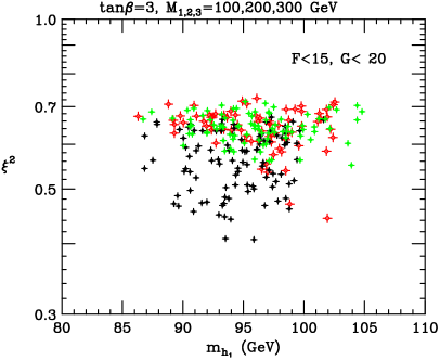
Figure 17: $\xi^{2}$ for $h=h_{1}$ as a function of $m_{a_{1}}$ and $m_{h_{1}}$ for points with $F<15$, $G<20$ and $|\cos\theta_{A}|<\cos\theta_{A}^{\rm max}(m_{a})$. These plots are those obtained using the described scanning procedure for $\tan\beta=3$.

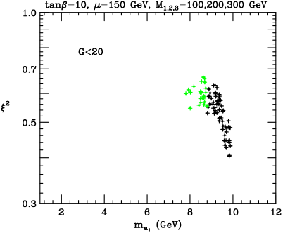
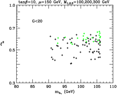
Figure 18: $\xi^{2}$ for $h=h_{1}$ as a function of $m_{a_{1}}$ and $m_{h_{1}}$ for points with $G<20$ and $|\cos\theta_{A}|<\cos\theta_{A}^{\rm max}(m_{a})$. These plots are those obtained using the “fixed-$\mu$” scanning procedure for $\tan\beta=10$.

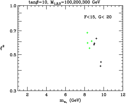
Figure 19: $\xi^{2}$ for $h=h_{1}$ as a function of $m_{a_{1}}$ and $m_{h_{1}}$ for points with $F<15$, $G<20$ and $|\cos\theta_{A}|<\cos\theta_{A}^{\rm max}(m_{a})$. These plots are those obtained using a “full scan” for $\tan\beta=10$.

Figure 20: $\xi^{2}$ for $h=h_{1}$ as a function of $m_{a_{1}}$ and $m_{h_{1}}$ for points with $G<20$ and $|\cos\theta_{A}|<\cos\theta_{A}^{\rm max}(m_{a})$. These plots are those obtained using the “fixed-$\mu$” scanning procedure for $\tan\beta=50$.

In addition, we have also considered $\xi^{2}$ expectations in scenarios with rather low $\tan\beta$. These were detailed in [33]. There, we performed fixed-$\mu$ scans as defined earlier, with the difference that at $\tan\beta=1.7$ and $\tan\beta=1.2$ we used different values for $M_{SUSY}$ and $A$ parameters, which values are indicated on the figures. At $\tan\beta=2$ we employed $M_{SUSY}=-A=300~{}{\rm GeV}$ as for the fixed-$\mu$ scans for $\tan\beta=3,10,50$.

The main distinguishing characteristic of the low $\tan\beta$ scenarios is that both $h_{1}$ and $h_{2}$ can be light with masses not far from $100~{}{\rm GeV}$, although there are certainly choices for the NMSSM parameters for which only $h_{1}$ is light while $h_{2}$ is much heavier. When $h_{2}$ is light, the charged Higgs $H^{\pm}$ can also have mass close to $100~{}{\rm GeV}$. Here, our interest is in the predictions for $\xi^{2}$.

Results for $\xi_{1}^{2}$ at $\tan\beta=2$ are rather similar to those found for higher $\tan\beta$, as shown in Fig. 21. In this figure, the blue $+$’s are all points that satisfy the NMHDECAY constraints — unlike the previous figures, color coding is not employed to distinguish different $m_{a_{1}}$ values. Results for $\xi_{2}^{2}$ are not shown; even when $m_{h_{2}}$ is close to $100~{}{\rm GeV}$, $\xi_{2}^{2}$ is quite small. This $\tan\beta=2$ case is similar to the $\tan\beta=3,10,50$ cases also in that it is almost always the case that $VV$ couples primarily to the $h_{1}$ so that when $m_{h_{1}}\leq 105~{}{\rm GeV}$ we have the “ideal” Higgs explanation of the precision electroweak data.

Figure 21: $\xi^{2}_{1}$ as a function of $m_{a_{1}}$ and $m_{h_{1}}$ for points with $G<20$ and $|\cos\theta_{A}|<\cos\theta_{A}^{\rm max}(m_{a_{1}})$ and $\tan\beta=2$. These plots are those obtained using a “fixed-$\mu$” scanning procedure with the $\mu$, $M_{SUSY}$ and $A$ parameters indicated on the figure. We have not indicated different $m_{a_{1}}$ mass ranges using different colors in these figures.

For $\tan\beta\mathrel{\raise 1.29167pt\hbox{$<$\kern-7.5pt\lower 4.30554pt\hbox{$\sim$}}}1.7$, there are some interesting new subtleties compared to $\tan\beta\mathrel{\raise 1.29167pt\hbox{$>$\kern-7.5pt\lower 4.30554pt\hbox{$\sim$}}}2$. Plots of $\xi_{1}^{2}$ of the $h_{1}$ and $\xi_{2}^{2}$ of $h_{2}$ appear in Figs. 22 and 23, respectively. In these plots, we follow the notation established in Ref. [33]. In detail, the blue $+$’s are all points that satisfy the NMHDECAY constraints. The red crosses single out those points for which $m_{h_{1}}<65~{}{\rm GeV}$. Yellow squares indicate points for which $BR(h_{1}\rightarrow a_{1}a_{1})<0.7$. In [33], there were also points indicated by green diamonds for which in addition the light CP-odd Higgs is primarily doublet-like, $\cos^{2}\theta_{A}>0.5$. However, these are absent from the present plots, not because of the improved $\cos\theta_{A}^{\rm max}$ limits from the recent BaBar data, but rather because of the $G<20$ requirement which very strongly disfavors large $|\cos\theta_{A}|$ at all $m_{a_{1}}$, including $m_{a_{1}}$ above $M_{\Upsilon(3S)}$. Of course, the BaBar data eliminates many points with $m_{a_{1}}<M_{\Upsilon(3S)}$ having $\cos^{2}\theta_{A}<0.5$, certainly more than in the analysis of [33].

Let us now discuss the $\tan\beta=1.7$ case in more detail. We first wish to discuss the extent to which the points that survive the NMHDECAY scans can be “ideal” in the precision electroweak sense. Defining

$$CV_{1}=g_{VVh_{1}}/g_{VVh_{SM}}\,,\qquad CV_{2}=g_{VVh_{2}}/g_{VVh_{SM}}\,,$$ (4)

then, noting that it is a good approximation to neglect any $h_{3}$ coupling to $VV$, one has the sum rule

$$CV_{1}^{2}+CV_{2}^{2}\simeq 1\,.$$ (5)

In this notation, the effective precision electroweak mass, $m_{eff}$, is given to very good approximation by

$$m_{eff}=m_{h_{1}}^{CV_{1}^{2}}m_{h_{2}}^{CV_{2}^{2}}\,.$$ (6)

In order to guarantee that all accepted points are ideal, we require as part of our $\tan\beta=1.7$ scan that $m_{eff}<100~{}{\rm GeV}$. Now, let us describe the associated plots. First, very low values of $m_{h_{1}}$ are possible (see the red crosses). These red cross points are such that $\xi_{1}^{2}$ and $\xi_{2}^{2}$ are comparable and both below $0.2$. Second, very few of the yellow square points (defined by $BR(h_{1}\rightarrow a_{1}a_{1})<0.7$) survive the ideal requirement. But, those that do have quite small $\xi_{1}^{2}$ and $\xi_{2}^{2}$. The run-of-the-mill blue $+$ points have somewhat larger $\xi_{1}^{2}\mathrel{\raise 1.29167pt\hbox{$<$\kern-7.5pt\lower 4.30554pt\hbox{$\sim$}}}0.4$ and somewhat smaller $\xi_{2}^{2}\mathrel{\raise 1.29167pt\hbox{$<$\kern-7.5pt\lower 4.30554pt\hbox{$\sim$}}}0.2$. Overall, the $4\tau$ final state in $h_{1}$ and $h_{2}$ decays typically has significantly smaller cross section for $\tan\beta=1.7$ as compared to $\tan\beta\mathrel{\raise 1.29167pt\hbox{$>$\kern-7.5pt\lower 4.30554pt\hbox{$\sim$}}}2$.

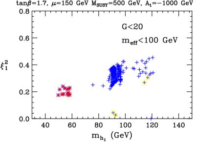
Figure 22: $\xi^{2}_{1}$ as a function of $m_{a_{1}}$ and $m_{h_{1}}$ for $\tan\beta=1.7$ points obtained from a fixed-$\mu$ scan after requiring $G<20$, $m_{eff}<100~{}{\rm GeV}$ and $|\cos\theta_{A}|<\cos\theta_{A}^{\rm max}(m_{a_{1}})$. The point notation is explained in the text.

d

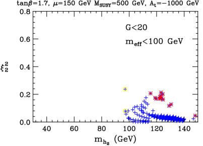
Figure 23: $\xi^{2}_{2}$ as a function of $m_{a_{1}}$ and $m_{h_{2}}$ for $\tan\beta=1.7$ points obtained from a fixed-$\mu$ scan after requiring $G<20$, $m_{eff}<100~{}{\rm GeV}$ and $|\cos\theta_{A}|<\cos\theta_{A}^{\rm max}(m_{a_{1}})$.

The lowest value of $\tan\beta$ consistent with maintaining perturbativity up to the GUT scale is $\tan\beta=1.2$. $\xi_{1}^{2}$ and $\xi_{2}^{2}$ plots for this case appear in Figs. 24 and 25, respectively. In this case, the effective $\xi_{1}^{2}$ values are mostly quite small. Relative to the $\tan\beta=1.7$ plots, the main thing that has changed is that $BR(a_{1}\rightarrow\tau^{+}\tau^{-})$ has declined substantially. The majority of the $a_{1}$ decays are into $gg$ and $c\overline{c}$, i.e. final states that are harder to constrain.

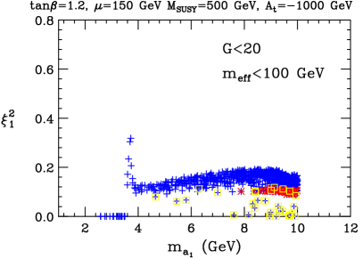
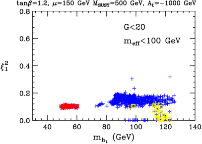
Figure 24: $\xi^{2}_{1}$ as a function of $m_{a_{1}}$ and $m_{h_{1}}$ for $\tan\beta=1.2$ points obtained from a fixed-$\mu$ scan after requiring $G<20$, $m_{eff}<100~{}{\rm GeV}$ and $|\cos\theta_{A}|<\cos\theta_{A}^{\rm max}(m_{a_{1}})$.

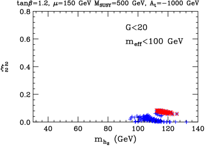
Figure 25: $\xi^{2}_{2}$ as a function of $m_{a_{1}}$ and $m_{h_{2}}$ for $\tan\beta=1.2$ points with $G<20$, $m_{eff}<100~{}{\rm GeV}$ and $|\cos\theta_{A}|<\cos\theta_{A}^{\rm max}(m_{a_{1}})$.

Of course, the knowledgeable reader will recognize that all the $\xi^{2}$ plots presented are aimed at comparing these NMSSM models to the new ALEPH analysis of the $4\tau$ final state [11]. According to the ALEPH analysis, to have $m_{h_{1}}\mathrel{\raise 1.29167pt\hbox{$<$\kern-7.5pt\lower 4.30554pt\hbox{$\sim$}}}100~{}{\rm GeV}$, $\xi^{2}_{1}\mathrel{\raise 1.29167pt\hbox{$<$\kern-7.5pt\lower 4.30554pt\hbox{$\sim$}}}0.52$ ($0.42$) is required if $m_{a_{1}}\sim 10~{}{\rm GeV}$ ($4~{}{\rm GeV}$). These limits rise rapidly with increasing $m_{h_{1}}$ — for $m_{h_{1}}=105~{}{\rm GeV}$ (the rough upper limit on $m_{h_{1}}$ such that electroweak finetuning remains quite small and precision electroweak constraints are fully satisfied) the ALEPH analysis requires $\xi^{2}\mathrel{\raise 1.29167pt\hbox{$<$\kern-7.5pt\lower 4.30554pt\hbox{$\sim$}}}0.85$ ($\mathrel{\raise 1.29167pt\hbox{$<$\kern-7.5pt\lower 4.30554pt\hbox{$\sim$}}}0.7$) at $m_{a_{1}}\sim 10~{}{\rm GeV}$ ($4~{}{\rm GeV}$). These limits are such that the easily viable NMSSM scenarios are ones: i) with $m_{a_{1}}$ below but fairly close to $2m_{B}$, which is, in any case, strongly preferred by minimizing the light-$a_{1}$ finetuning measure $G$; and/or ii) with $\tan\beta$ relatively small ($\mathrel{\raise 1.29167pt\hbox{$<$\kern-7.5pt\lower 4.30554pt\hbox{$\sim$}}}2$).  These are also the scenarios for which Upsilon constraints are either weak or absent. In particular, we note the following: a) all $\tan\beta\leq 2$ cases provide $m_{h_{1}}\leq 100~{}{\rm GeV}$ scenarios that escape the ALEPH limits; b) there are a few $G<20$, $\tan\beta=3$ scenarios with $m_{h_{1}}$ as large as $98~{}{\rm GeV}$ and $99~{}{\rm GeV}$ and with $\xi^{2}$ essentially equal to the ALEPH limits of $\xi^{2}\leq 0.42$ and $\xi^{2}\leq 0.45$ applicable at these respective $m_{h_{1}}$ values; c) $\tan\beta=10$ ideal scenarios easily allow for $m_{h_{1}}\sim 100-105~{}{\rm GeV}$ (because the tree-level Higgs mass is larger at $\tan\beta=10$ than at $\tan\beta=3$) and at $m_{a_{1}}\mathrel{\raise 1.29167pt\hbox{$<$\kern-7.5pt\lower 4.30554pt\hbox{$\sim$}}}2m_{B}$ many $m_{h_{1}}\mathrel{\raise 1.29167pt\hbox{$>$\kern-7.5pt\lower 4.30554pt\hbox{$\sim$}}}100~{}{\rm GeV}$ points have $\xi^{2}<0.5$ in the fixed-$\mu$ scan and a few of the full-scan points have $\xi^{2}<0.6$ for $m_{h_{1}}\sim 105~{}{\rm GeV}$, both of which are below the $m_{a_{1}}=10~{}{\rm GeV}$ ALEPH upper limits on $\xi^{2}$ of 0.52 at $m_{h_{1}}\sim 100~{}{\rm GeV}$ and $0.85$ at $m_{h_{1}}=105~{}{\rm GeV}$; d) at $\tan\beta=50$ there are some $G<20$ points with $m_{h_{1}}\sim 100~{}{\rm GeV}$ and $m_{a_{1}}\mathrel{\raise 1.29167pt\hbox{$<$\kern-7.5pt\lower 4.30554pt\hbox{$\sim$}}}2m_{B}$ having $\xi^{2}$ below the $0.52$ ALEPH limit. Finally, we note that for the entire range of Higgs masses studied the ALEPH limits were actually $\sim 2\sigma$ stronger than expected. Thus, it is not completely unreasonable to consider the possibility that the weaker expected limits should be employed. These weaker limits for example allow $\xi^{2}$ as large as $0.52$ at $m_{h_{1}}\sim 95~{}{\rm GeV}$ and $0.9$ for $m_{h_{1}}\sim 100~{}{\rm GeV}$. These weaker limits allow ample room for the majority of the $m_{a_{1}}\mathrel{\raise 1.29167pt\hbox{$<$\kern-7.5pt\lower 4.30554pt\hbox{$\sim$}}}2m_{B}$ ideal Higgs scenarios.

6 Conclusions

In this paper, we have updated the constraints on the NMSSM ideal Higgs scenarios in which $h_{1}$ (and for low $\tan\beta$, also possibly $h_{2}$) has mass $\mathrel{\raise 1.29167pt\hbox{$<$\kern-7.5pt\lower 4.30554pt\hbox{$\sim$}}}105~{}{\rm GeV}$ and decays largely (but not entirely) via $h_{1}\rightarrow a_{1}a_{1}\rightarrow\tau^{+}\tau^{-}\tau^{+}\tau^{-}$. Such low mass(es) for the Higgs boson(s) with large $VV$ coupling are strongly preferred by precision electroweak data and are also strongly preferred in order to minimize electroweak finetuning. Indeed, all the NMSSM points plotted in this paper have effective precision electroweak mass below $\sim 105~{}{\rm GeV}$. The new data that constrains such scenarios derives from $\Upsilon_{3S}\rightarrow\gamma\mu^{+}\mu^{-}$ and $\gamma\tau^{+}\tau^{-}$ decay data from BaBar and ALEPH studies of the $e^{+}e^{-}\rightarrow Z4\tau$ final state. The latter was employed by ALEPH to place limits as a function of $m_{h_{1}}$ and $m_{a_{1}}$ on the quantity $\xi^{2}\equiv{\sigma(h_{1})\over\sigma(h_{SM})}BR(h_{1}\rightarrow a_{1}a_{1})\left[BR(a_{1}\rightarrow\tau^{+}\tau^{-})\right]^{2}$. Although these new constraints are significant, there is still ample room for the ideal Higgs scenarios, especially if $\tan\beta$ is small and $m_{a_{1}}\mathrel{\raise 1.29167pt\hbox{$<$\kern-7.5pt\lower 4.30554pt\hbox{$\sim$}}}2m_{B}$ (the latter region being that for which the “light-$a_{1}$” finetuning measure is minimal and also $BR(a_{1}\rightarrow\tau^{+}\tau^{-})$ is somewhat suppressed). For $\tan\beta\geq 3$, it is only the $m_{a_{1}}\mathrel{\raise 1.29167pt\hbox{$<$\kern-7.5pt\lower 4.30554pt\hbox{$\sim$}}}2m_{B}$ points that can escape the ALEPH $\xi^{2}$ limits. The case of $\tan\beta=3$ is the most marginal with only a few NMSSM points with $m_{h_{1}}\leq 99~{}{\rm GeV}$ (the rough upper limit on $m_{h_{1}}$ at $\tan\beta=3$) having $\xi^{2}$ essentially equal to the ALEPH limit at a given $m_{h_{1}}$. For $\tan\beta=10$, one finds scenarios with $m_{h_{1}}\sim 100-105~{}{\rm GeV}$ and $\xi^{2}\sim 0.43$ when $m_{a_{1}}\mathrel{\raise 1.29167pt\hbox{$<$\kern-7.5pt\lower 4.30554pt\hbox{$\sim$}}}2m_{B}$, which $\xi^{2}$ is well below the ALEPH limit of $\sim 0.52-0.85$ for such $m_{h_{1}}$ and $m_{a_{1}}$. At $\tan\beta=50$, although our scanning statistics were limited, we found points with $m_{h_{1}}\sim 100~{}{\rm GeV}$ and $m_{a_{1}}\mathrel{\raise 1.29167pt\hbox{$<$\kern-7.5pt\lower 4.30554pt\hbox{$\sim$}}}2m_{B}$ having $\xi^{2}$ below the $0.52$ ALEPH limit. (We note that the ALEPH limits are significantly stronger than the ALEPH collaboration was expecting. If one were to use expected limits instead then the $\tan\beta\geq 3$ scenarios would be much less constrained.) For $\tan\beta\mathrel{\raise 1.29167pt\hbox{$<$\kern-7.5pt\lower 4.30554pt\hbox{$\sim$}}}2$, the ideal-Higgs NMSSM scenarios are not particularly constrained by the ALEPH limits. In particular, for $\tan\beta=2,1.7,1.2$ one finds $m_{h_{1}}\leq 100~{}{\rm GeV}$ scenarios with $\xi^{2}\mathrel{\raise 1.29167pt\hbox{$<$\kern-7.5pt\lower 4.30554pt\hbox{$\sim$}}}0.32,0.23,0.15$, respectively. The lower $\xi^{2}$ values arise because these lower $\tan\beta$ values have increasingly reduced $BR(a_{1}\rightarrow\tau^{+}\tau^{-})$, which, in turn, is due to increasingly larger values of $BR(a_{1}\rightarrow gg+c\overline{c})$. Such $\xi^{2}$ values are completely consistent with the ALEPH limits.

The Tevatron and LHC discovery prospects for the Higgs bosons in the low-$\tan\beta$ scenarios have yet to be fully analyzed. Searches for the $h_{1}$ and the $a_{1}$ using the $a_{1}\rightarrow\tau^{+}\tau^{-}$ and $a_{1}\rightarrow\mu^{+}\mu^{-}$ decay modes will certainly become more difficult as these branching ratios decline with decreasing $\tan\beta$. Such search modes include: direct (vs. coming from $h_{1}\rightarrow a_{1}a_{1}$) detection of the $a_{1}$ at the Tevatron and LHC in the $gg\rightarrow a_{1}\rightarrow\mu^{+}\mu^{-}$ channel [27]; searches for $gg\rightarrow h_{1}\rightarrow a_{1}a_{1}\rightarrow\tau^{+}\tau^{-}\tau^{+}\tau^{-}$, $\tau^{+}\tau^{-}\mu^{+}\mu^{-}$ and/or $\mu^{+}\mu^{-}\mu^{+}\mu^{-}$ at the Tevatron [34] and LHC [35]; and LHC detection of $pp\rightarrow pph_{1}$ with $h_{1}\rightarrow a_{1}a_{1}\rightarrow\tau^{+}\tau^{-}\tau^{+}\tau^{-}$ [36]. Backgrounds in the increasingly important channels with $a_{1}\rightarrow gg+c\overline{c}$ will undoubtedly be much larger and will make discovery employing these latter $a_{1}$ decay modes quite difficult.

As part of the NMSSM study, we first obtained updated limits on the $ab\overline{b}$ coupling (assuming $C_{ab\overline{b}}=C_{a\tau^{-}\tau^{+}}=C_{a\mu^{-}\mu^{+}}$) that are applicable in a wide variety of model contexts. The main improvements in these general limits result from recent BaBar data.

Finally, one should not forget that the NMSSM is only the simplest model of a general category of SUSY models having one or more singlet scalar superfields in addition to the usual two-doublet scalar superfields. Such models are generically very attractive in that they allow for an NMSSM-like solution to the $\mu$ problem, while maintaining coupling constant unification and RGE electroweak symmetry breaking as in the MSSM. In addition, models with more than one extra singlet scalar superfield will allow one or more light Higgs bosons with SM-like couplings to $VV$ (a scenario having excellent agreement with precision electroweak constraints and minimal electroweak finetuning) that can escape Upsilon and LEP limits more easily than the NMSSM by virtue of multiple decays channels of the Higgs$\rightarrow a_{k}a_{j}$, …type.

References

[1]
R. Dermisek and J. F. Gunion,
Phys. Rev. Lett. 95, 041801 (2005)
[arXiv:hep-ph/0502105].
[2]
R. Dermisek and J. F. Gunion,
Phys. Rev. D 73, 111701 (2006)
[arXiv:hep-ph/0510322].
[3]
R. Dermisek and J. F. Gunion,
Phys. Rev. D 75, 075019 (2007)
[arXiv:hep-ph/0611142].
[4]
R. Dermisek and J. F. Gunion,
Phys. Rev. D 76, 095006 (2007)
[arXiv:0705.4387 [hep-ph]].
[5]
S. Chang, P. J. Fox and N. Weiner,
JHEP 0608, 068 (2006)
[arXiv:hep-ph/0511250].
[6]
S. Chang, R. Dermisek, J. F. Gunion and N. Weiner,
arXiv:0801.4554 [hep-ph].
[7]
J. F. Gunion,
arXiv:0808.2509 [hep-ph].
[8]
F. Domingo, U. Ellwanger, E. Fullana, C. Hugonie and M. A. Sanchis-Lozano,
JHEP 0901, 061 (2009)
[arXiv:0810.4736 [hep-ph]].
[9]
B. Aubert et al. [BABAR Collaboration],
Phys. Rev. Lett. 103, 181801 (2009)
[arXiv:0906.2219 [hep-ex]].
[10]
B. Aubert et al. [BABAR Collaboration],
Phys. Rev. Lett. 103, 081803 (2009)
[arXiv:0905.4539 [hep-ex]].
[11]
The ALEPH Collaboration,
arXiv:1003.0705 [hep-ex].
[12]
J. R. Ellis, J. F. Gunion, H. E. Haber, L. Roszkowski and F. Zwirner,
Phys. Rev. D 39, 844 (1989).
[13]The Higgs Hunter’s Guide,
John F. Gunion, Howard E. Haber, Gordon Kane, Sally Dawson. 1990.
Series: Frontiers in Physics, 80; QCD161:G78
[14]
U. Ellwanger, J. F. Gunion and C. Hugonie,
JHEP 0502, 066 (2005)
[arXiv:hep-ph/0406215].
[15]
U. Ellwanger and C. Hugonie,
Comput. Phys. Commun. 175, 290 (2006)
[arXiv:hep-ph/0508022].
[16]
L. J. Hall, R. Rattazzi and U. Sarid,
Phys. Rev. D 50, 7048 (1994)
[arXiv:hep-ph/9306309].
[17]
M. S. Carena, M. Olechowski, S. Pokorski and C. E. M. Wagner,
Nucl. Phys. B 426, 269 (1994)
[arXiv:hep-ph/9402253].
[18]
D. M. Pierce, J. A. Bagger, K. T. Matchev and R. j. Zhang,
Nucl. Phys. B 491, 3 (1997)
[arXiv:hep-ph/9606211].
[19]
A. Djouadi, J. Kalinowski and M. Spira,
Comput. Phys. Commun. 108, 56 (1998)
[arXiv:hep-ph/9704448].
[20]
R. Dermisek, J. F. Gunion and B. McElrath,
Phys. Rev. D 76, 051105 (2007)
[arXiv:hep-ph/0612031].
[21]
W. Love et al. [CLEO Collaboration],
Phys. Rev. Lett. 101, 151802 (2008)
[arXiv:0807.1427 [hep-ex]].
[22]
M. Drees and K. i. Hikasa,
Phys. Rev. D 41, 1547 (1990).
[23]
M. A. Sanchis-Lozano,
Mod. Phys. Lett. A 17, 2265 (2002)
[arXiv:hep-ph/0206156].
M. A. Sanchis-Lozano,
Int. J. Mod. Phys. A 19, 2183 (2004)
[arXiv:hep-ph/0307313].
E. Fullana and M. A. Sanchis-Lozano,
Phys. Lett. B 653, 67 (2007)
[arXiv:hep-ph/0702190].
M. A. Sanchis-Lozano,
arXiv:0709.3647 [hep-ph].
[24]
G. Abbiendi et al. [OPAL Collaboration],
Eur. Phys. J. C 23, 397 (2002)
[arXiv:hep-ex/0111010].
[25]
The Delphi Collaboration, ICHEP 2002, DELPHI 2002-037-CONF-571. We
employ Table 20 — these are very close to
those appearing in the figures of
J. Abdallah et al. [DELPHI Collaboration],
Eur. Phys. J. C 38, 1 (2004)
[arXiv:hep-ex/0410017].
[26]
T. Aaltonen et al. [CDF Collaboration],
arXiv:0906.1014 [hep-ex].
[27]
R. Dermisek and J. F. Gunion,
arXiv:0911.2460 [hep-ph].
[28]
G. Apollinari et al.,
Phys. Rev. D 72, 092003 (2005)
[arXiv:hep-ex/0507044].
[29]
T. Aaltonen et al. [CDF Collaboration],
Eur. Phys. J. C 62, 319 (2009)
[arXiv:0903.2060 [hep-ex]].
[30]
R. Dermisek,
arXiv:0806.0847 [hep-ph].
[31]
R. Dermisek,
AIP Conf. Proc. 1078, 226 (2009)
[arXiv:0809.3545 [hep-ph]].
[32]
K. J. Bae, R. Dermisek, D. Kim, H. D. Kim and J. H. Kim,
arXiv:1001.0623 [hep-ph].
[33]
R. Dermisek and J. F. Gunion,
Phys. Rev. D 79, 055014 (2009)
[arXiv:0811.3537 [hep-ph]].
[34]
V. M. Abazov et al. [D0 Collaboration],
Phys. Rev. Lett. 103, 061801 (2009)
[arXiv:0905.3381 [hep-ex]].
[35]
M. Lisanti and J. G. Wacker,
Phys. Rev. D 79, 115006 (2009)
[arXiv:0903.1377 [hep-ph]].
[36]
J. R. Forshaw, J. F. Gunion, L. Hodgkinson, A. Papaefstathiou and A. D. Pilkington,
JHEP 0804, 090 (2008)
[arXiv:0712.3510 [hep-ph]].