Bolometric correction and spectral energy distribution of cool stars in Galactic clusters

Abstract

In this work we have investigated the relevant trend of the bolometric correction (BC) at the cool-temperature regime of red giant stars and its possible dependence on stellar metallicity. Our analysis relies on a wide sample of optical-infrared spectroscopic observations, along the 3500 Å $\Rightarrow 2.5\mu$m wavelength range, for a grid of 92 red giant stars in five (3 globular + 2 open) Galactic clusters, along the full metallicity range covered by the bulk of the stars, $-2.2\leq[Fe/H]\leq+0.4$.

Synthetic $BVR_{c}I_{c}JHK$ photometry from the derived spectral energy distributions allowed us to obtain robust temperature (T_eff) estimates for each star, within $\pm 100$ K or less. According to the appropriate temperature estimate, black-body extrapolation of the observed spectral energy distribution (SED) allowed us to assess the unsampled flux beyond the wavelength limits of our survey. For the bulk of our red giants, this fraction amounted to 15% of the total bolometric luminosity, a figure that raises up to 30% for the coolest targets (T${}_{\rm eff}\lesssim 3500$ K). Allover, we trust to infer stellar M_bol values with an internal accuracy of a few percent. Even neglecting any correction for lost luminosity etc. we would be overestimating M_bol by $\la 0.3$ mag, in the worst cases. Making use of our new database, we provide a set of fitting functions for the V and K BC vs. T_eff and vs. $(B-V)$ and $(V-K)$ broad-band colors, valid over the interval $3300~{}{\rm K}\leq{\rm T}_{\rm eff}\leq 5000$ K, especially suited for Red Giants.

The analysis of the BC_V and BC_K estimates along the wide range of metallicity spanned by our stellar sample show no evident drift with [Fe/H]. Things may be different for the B-band correction, where the blanketing effects are more and more severe. A drift of $\Delta(B-V)$ vs. [Fe/H] is in fact clearly evident from our data, with metal-poor stars displaying a “bluer” $(B-V)$ with respect to the metal-rich sample, for fixed T_eff.

Our empirical bolometric corrections are in good overall agreement with most of the existing theoretical and observational determinations, supporting the conclusion that (a) $BC_{K}$ from the most recent studies are reliable within $\la\pm 0.1$ over the whole color/temperature range considered in this paper, and (b) the same conclusion apply to $BC_{V}$ only for stars warmer than $\simeq 3800$ K. At cooler temperatures the agreement is less general, and MARCS models are the only ones providing a satisfactory match to observations, in particular in the $BC_{V}$ vs. $(B-V)$ plane.

1 Introduction

A physical assessment of the bolometric emission of stars is a mandatory step for any attempt to self-consistently link observations and theoretical predictions of stellar evolution. The importance of this comparison actually reverberates into a wide range of primary astrophysical questions, ranging from the validation of the reference input physics for nuclear reactions in the stellar interiors to the study of integrated spectrophotometric properties of distant galaxies, through stellar population synthesis models.

By definition, the effective temperature (T_eff) and physical size ($R$) of a star provide the natural constraint to its emerging flux, as $L\propto R^{2}\,T_{\rm eff}^{4}$. If $L$ is a known property for a star, then we could physically “rescale” the spectral energy distribution (SED), and infer, from the observed flux, the distance of the body, $d$, or its absolute size ($R$), through a measure of the apparent angular extension, $\theta=(R/d)^{2}\propto L\,T_{\rm eff}^{-4}\,d^{-2}$ (Ridgway et al., 1980; Dyck et al., 1996; Perrin et al., 1998; Richichi et al., 1998).

As well known, however, $L$ cannot, in principle, be directly measured, requiring for this task an ideal detector equally sensitive to the whole spectral range. The lack of this crucial piece of information is often palliated by indirect observing methods, trying to pick up the bulk of stellar emission through broad-band photometry within the appropriate spectral range according to target temperature. Relying on this approach, Johnson (1966) derived the bolometric vs. temperature scale for red giant stars, while Code et al. (1976) explored the same relation for hot early-type stars, through satellite-borne UV observations. As an alternative way, many authors tried a fully theoretical assessment of the problem, by studying the $f_{\rm bol}$ vs. $f_{\rm\lambda}$ relationship on the basis of model grids of stellar atmospheres and replacing observations with synthetic photometry directly computed on the theoretical SED (Bertone et al., 2004; Bessell, Castelli, & Plez, 1998).

Rather than focussing on luminosity, Wesselink (1969) originally proposed a further application of this method, just looking at the bolometric surface brightness, namely $\mu=f_{\rm bol}/\theta^{2}$, to lead to a refined temperature scale of stars in force of the fundamental relationship $\mu=\sigma\,T_{\rm eff}^{-4}$ ($\sigma$ being the Stefan-Boltzmann constant). The so-called surface-brightness technique, then better recognized as the IR-flux method (IRFM), has been extensively applied to the study of red giant and supergiant stars (Blackwell, Shallis, & Selby, 1979; di Benedetto & Rabbia, 1987; Blackwell & Lynas-Gray, 1994; Alonso, Arribas, & Martínez-Roger, 1999; Ramírez & Meléndez, 2005; González Hernández & Bonifacio, 2009) taking advantage of its distance-independent results, providing to match the angular measure of stellar radii with the estimate of the bolometric flux from infrared observations, i.e. $\mu=(f_{\rm bol}/f_{\rm IR})f_{\rm IR}$.

Although in different forms, all the previous methods used theoretical models of stellar atmospheres to derive the appropriate “correcting factor” ${\cal R}=f_{\rm bol}/f(\lambda)$ and convert observed or synthetic monochromatic magnitudes, $m(\lambda)$ to the bolometric scale.

Taking the Sun as a reference source for our calibration, we could write more explicitely:

$$[m_{\rm bol}-m(\lambda)]-[m_{\rm bol}-m(\lambda)]_{\odot}=-2.5\,\log({\cal R/R}_{\odot})$$ (1)

Equation (1) actually leads to the straight definition of bolometric correction, $BC(\lambda)$, namely

$$BC(\lambda)=(m_{\rm bol}-m(\lambda))=-2.5\,\log{\cal R}+BC(\lambda)_{\odot}$$ (2)

Aside from the historical definition, that originally considered BC only to photographic ($m_{\rm pg}$) or visual ($m_{V}$) magnitudes (Kuiper, 1938), one can nowadays easily extend the definition to any waveband. A careful analysis of eq. (2) makes clear some important properties of $BC$: i) the value of $\cal R$ is a composite function of stellar fundamental parameters, namely ${\cal R}={\cal R}(T_{\rm eff},\log g,[X/H])$ so that, for fixed effective temperature, $BC$ may display some dependence on stellar gravity ($g$) and chemical composition ($[X/H]$); ii) the value of $\cal R$ (and, accordingly, of $BC$) is minimum when our observations catch the bulk of stellar luminosity. For this reason, high values of $BC_{V}$ must be expected when observing for instance cool giant stars in the $V$ band, or hot O-B stars in the infrared $K$ band. iii) The definition of the $BC$ scale strictly depends on the assumed reference value for the Sun, that therefore must univocally fix the “zero point” of the scale (Bessell, Castelli, & Plez, 1998).

In this framework, we want to tackle here the central question of the possible $BC$ dependence on stellar metallicity. This effect could be of special importance, in fact, in order to more confidently set the bolometric vs. temperature scale for cool red giants, where the intervening absorption of diatomic (TiO in primis) and triatomic (H₂O) molecules heavily modulate the stellar SED with sizeable effects on optical and NIR magnitudes (e.g. Gratton et al., 1982; Bertone et al., 2008). As a matter of fact, still nowadays the many efforts devoted to the definition of the $BC$ vs. $\log T_{\rm eff}$ relationship led to non univocal conclusions, with large discrepancies among the different sources in the literature as far as stars of K spectral type or later are concerned (Flower, 1975, 1977; Bessell & Wood, 1984; Houdashelt, Bell, & Sweigart, 2000; Bertone et al., 2004; Worthey & Lee, 2006).

This issue has actually an even more important impact on the study of the integrated spectrophotometric properties of resolved and unresolved stellar systems, as red giants and other Post-main sequence (PMS) stars provide a prevailing fraction (2/3 or more, Buzzoni, 1989) of the total luminosity of the population. A fair definition of the $BC$ scale becomes therefore of paramount importance to self-consistently convert theoretical H-R and observed c-m diagrams of a stellar population (Flower, 1996; VandenBerg & Clem, 2003) and more confidently assess the physical contribution of the different stellar classes.

A study of the $BC$ dependence on metal abundance has been previously attempted by many authors mainly relying on a fully theoretical point of view to exploit the obvious advantage of stellar models to account in a controlled way for a global or selective change of metal abundance. In this regard, Tripicco & Bell (1995) and Cassisi et al. (2004), among others, tried to explore the effect of $\alpha$ elements enhancement (namely O, Mg, Ca, Ti etc.) in stellar SED, while Girardi et al. (2007) focussed on the possible impact of Helium abundance on $BC$. As a major drawback of these efforts, however, one has to report the admitted limit of model atmospheres in accurately describe the spectrophotometric properties of K- and M-type stars, that are cooler than 4000 K (see Bertone et al., 2008, on this important point).

On the other hand, a fully empirical approach has been devised by Montegriffo et al. (1998) and Alonso, Arribas, & Martínez-Roger (1999), among others, trying to reconstruct stellar SED, and therefrom infer the bolometric flux, $f_{\rm bol}$, through optical broad-band photometry of stars in the Galactic field or in globular clusters. A recognized limit of these studies is, however, that they may suffer from the lack of coverage of the stellar parameter space offered by the observations. Moreover, as far as the cool-star sequence is concerned, optical multicolor photometry, alone, partially misses the bulk of stellar emission (more centered toward the NIR spectral window); in addition, by converting broad-band magnitudes into monochromatic flux densities, the stellar SED is reconstructed at very poor spectral resolution, thus possibly loosing important features that may bias the inferred bolometric energy budget.

On this line, however, we want to further improve the analysis proposing here more complete spectroscopic observations for a large grid of red-giant stars in several Galactic clusters along the entire metallicity scale from very metal-poor (i.e. $[Fe/H]\simeq-2.2$ dex) to super-solar ($[Fe/H]\simeq+0.4$ dex) stellar populations. Our observations span the whole optical and NIR wavelength range, thus allowing a quite accurate shaping of stellar SED. As we will demonstrate in the following of our discussion, our procedure allowed us to sample about 70-90 % of the total emission of our sample stars, thus leading to a virtually direct measure of $f_{\rm bol}$, even for M-type stars as cool as 3500 K.

We will arrange our discussion by presenting, in Sec. 2, our stellar database together with further available information in the literature. The analysis of the observing material will be assessed in more detail in Sec. 3, while in Sec. 4 we will derive the SED for the whole sample leading to an estimate of the effective temperature and bolometric correction for each star. The discussion of the inferred BC-color-temperature scale will be the focus of Sec. 5, especially addressing the possible dependence of BC on stellar metallicity. The comparison of our results with other relevant BC calibration in the literature will also be carried out in this section, while in Sec. 6 we will summarize the main conclusions of our work.

2 Cluster database selection

As we mainly aim at probing the impact of metallicity on the BC of stars at the low-temperature regime, a demanding constraint to set up our target sample was to explore a range as wide as possible in [Fe/H], and pick up red giant stars with accurate measurements of their metallicity. The cluster population in the Galaxy naturally provided the ideal environment for our task. By combining globular and open clusters one can easily span the whole metallicity range pertinent to Pop I and II stars in our and in external galaxies. We therefore selected five template systems, namely the three metal-poor globular clusters M15, M2 and M71, and two metal-rich open clusters NGC 188 and NGC 6791 such as to let metallicity span almost three orders of magnitude, from [Fe/H] $=-2.3$ up to +0.4.

For each cluster, a subset of $\sim 20$ suitable targets have then been identified among the brightest and coolest red giants from the 2MASS infrared c-m diagram (Skrutskie et al., 2006). In assembling the dataset we also took care of picking up those objects out of more severely crowded regions of the clusters, and clearly recognizable in bright asterisms such as to reduce the chance of misidentification at the telescope.

The final set of target stars is summarized, for each cluster, in the five panels of Fig. 1 and in the series of Tables 1 to 5. We eventually considered 92 stars in total, of which 21 are in M15, 18 in M2, 17 in M71, 16 in NGC 188, and 20 in NGC 6791, respectively. For each star, the tables always report the 2MASS id number (col. 1) and the alternative cross-identification, according to other reference photometric catalogs, when available. The 2MASS J2000 coordinates on the sky and the corresponding $J,H,K$ magnitudes are also always reported, together with a compilation of $B,V,R_{c},I_{c}$ observed magnitudes according to the best reference catalogs for each cluster, as reported in the literature. When required, dereddened apparent magnitudes have been computed according to the color excess $E(B-V)$ as labelled in the header of each table.

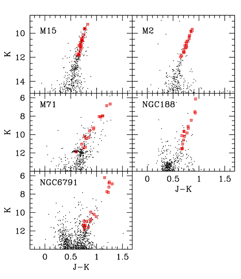
Figure 1: Apparent c-m diagram of the five clusters included in our analysis, according to 2MASS J and K photometry. Big squares along the red giant branch mark the selected targets in our sample.

3 Observations and data reduction

Spectroscopic observations of our stellar sample have been collected during several runs between June and October 2003 at the 3.5m Telecopio Nazionale Galileo (TNG) of the Roque de los Muchachos Observatory, at La Palma (Canary Islands, Spain). A summary of the logbook can be found in Table 6.

Optical spectroscopy was carried out with the LRS FOSC camera; a composite spectrum was collected for each target by matching a blue (grism LRB along the $\lambda\lambda 3500-8800$ Å wavelength range) and a red setup (grism LRR, between $\lambda\lambda 4500-10300$ Å). In both cases the grisms provided a dispersion of 2.8 Å px^-1 on a $2048\times 2048$ thinned and back-illuminated Loral CCD, with a 13.5$\mu$m pixel size. In order to collect the entire flux from target stars, we observed through a 5″wide slit; this condition actually made spectral resolution to be eventually constrained by the seeing figure (typically about 1-1.5″along the different nights), thus ranging between 10 and 15 Å (FWHM). This is equivalent to a value of $R=\lambda/\Delta\lambda$ between 600-1000. Whenever possible, and avoiding severe crowding conditions of the target fields, the longslit was located at the parallactic angle. Wavelength calibration and data reductions were performed following standard procedures.

Table 1: Cluster properties and stellar database for cluster M 15

M 15:           E(B–V) = 0.10           [Fe/H] = –2.26
ID			$\alpha$	$\delta$	B	V		Ic		J	H	K
(a)	(b)	(c)	(J2000.0)		(b)	(b)	(c)	(b)	(c)	(a)	(a)	(a)
21300002+1209182	165	71	21:30:00.02	12:09:18.24	15.334	14.395	14.3460	13.330	13.2709	12.479	11.926	11.824
21295705+1208531	959	6	21:29:57.06	12:08:53.11	14.549	13.426	13.4946	12.144	12.2129	11.282	10.691	10.573
21295532+1210327	337	60	21:29:55.33	12:10:32.80	15.229	14.313	14.3694	13.165	13.2132	12.452	11.899	11.786
21300090+1208571	558	461	21:30:00.91	12:08:57.13	14.092	12.700	12.9683	11.281	11.4637	10.383	9.759	9.605
21295473+1208592	330	25	21:29:54.73	12:08:59.24	14.821	13.691	13.7581	12.444	12.5006	11.591	11.065	10.906
21300461+1210327	369		21:30:04.62	12:10:32.73	14.851	13.836				11.858	11.272	11.165
21295560+1212422	533	665	21:29:55.61	12:12:42.29	14.562	13.459	13.5218		12.2237	11.336	10.723	10.609
21300514+1210041	372		21:30:05.15	12:10:04.18	15.186	14.288				12.430	11.929	11.776
21295836+1209020		166	21:29:58.37	12:09:02.01			13.8205		12.5987	11.700	11.112	11.042
21295618+1210179		631	21:29:56.18	12:10:17.93			12.7694		11.3768	10.414	9.781	9.649
21295739+1209056		7	21:29:57.39	12:09:05.69			13.7397		12.5054	11.632	11.070	10.948
21300097+1210375		65	21:30:00.98	12:10:37.60			13.8739		12.6289	11.726	11.171	11.017
21300431+1210561	368		21:30:04.32	12:10:56.16	14.649	13.559				11.459	10.893	10.757
21301049+1210061	621		21:30:10.49	12:10:06.18	14.563	13.406				11.151	10.562	10.438
21300739+1210330	604		21:30:07.40	12:10:33.06	14.961	13.986				11.964	11.399	11.264
21300569+1210156			21:30:05.70	12:10:15.68						12.156	11.596	11.480
21300553+1208553			21:30:05.54	12:08:55.35						12.357	11.835	11.719
21295756+1209438			21:29:57.57	12:09:43.85						10.096	9.429	9.269
21295082+1211301			21:29:50.83	12:11:30.18						11.326	10.725	10.612
21295881+1209285		59	21:29:58.82	12:09:28.59			14.5465		13.5061	11.088	10.568	10.353
21295716+1209175		273	21:29:57.17	12:09:17.52			13.1662		11.7880	10.867	10.220	10.112

^(a) from 2MASS;
^(b) from Cohen, Briley, & Stetson (2005);
^(c) from Rosenberg et al. (2000)

The optical spectra have then been accompanied by the corresponding observations taken at infrared wavelength with the NICS camera at the Nasmyth focus of the TNG. The camera was coupled with a Rockwell 1024$\times$1024 Hawaii-1 HgCdTe detector. We took advantage of NICS unique design using the Amici grism coupled with two slits 0.5″and 5″wide, the latter being used for a complete flux sampling of the target stars. The spectra cover the entire wavelength range from 8000 Å to 2.5 $\mu$m at a resolving power (for a 0.5″slit) which varies between $R=80$ and 140 along the spectrum. In acquiring spectra, background subtraction and flat-fielding correction were eased by a standard dithering procedure on target images, while the wavelength calibration directly derived from the standard reference table providing the dispersion relation of the system. The Midas ESO package, and specifically its Longslit routine set, has been used for the whole reduction procedure, both for optical and infrared spectra.

Table 2: Cluster properties and stellar database for cluster M 2^(a)

M 2:           E(B–V) = 0.06           [Fe/H] = –1.62
ID	$\alpha$	$\delta$	J	H	K
	(J2000.0)
21333827-0054569	21:33:38.28	–00:54:56.92	10.542	9.827	9.672
21333095-0052154	21:33:30.96	–00:52:15.47	11.568	10.952	10.814
21332468-0044252	21:33:24.69	–00:44:25.21	12.549	12.006	11.886
21331771-0047273	21:33:17.71	–00:47:27.31	10.665	9.961	9.821
21331723-0048171	21:33:17.24	–00:48:17.10	11.112	10.429	10.301
21331790-0048198	21:33:17.91	–00:48:19.82	11.746	11.103	11.017
21331854-0051563	21:33:18.55	–00:51:56.33	11.779	11.137	11.019
21331948-0051034	21:33:19.49	–00:51:03.42	11.963	11.299	11.214
21331923-0049058	21:33:19.23	–00:49:05.84	12.280	11.695	11.579
21332588-0046004	21:33:25.89	–00:46:00.44	12.313	11.756	11.600
21333668-0051058	21:33:36.68	–00:51:05.89	10.730	10.026	9.880
21333520-0046089	21:33:35.21	–00:46:08.91	10.993	10.324	10.174
21333488-0047572	21:33:34.88	–00:47:57.25	11.265	10.589	10.455
21333593-0049224	21:33:35.94	–00:49:22.44	11.420	10.750	10.650
21333432-0051285	21:33:34.33	–00:51:28.50	11.490	10.828	10.722
21332531-0052511	21:33:25.32	–00:52:51.17	11.938	11.300	11.203
21333109-0054522	21:33:31.09	–00:54:52.28	12.086	11.526	11.376
21333507-0051097	21:33:35.07	–00:51:09.72	12.609	12.056	11.962

^(a) all the data are from 2MASS;

Table 3: Cluster properties and stellar database for cluster M 71

M 71:          E(B–V) = 0.25          [Fe/H] = –0.73
ID			$\alpha$	$\delta$	B	V		Ic	J	H	K
(a)	(b)	(c)	(J2000.0)		(b)	(b)	(c)	(c)	(a)	(a)	(a)
19535325+1846471	2672	256	19:53:53.25	18:46:47.13	13.905	12.314	12.2085	10.3988	9.090	8.197	8.040
19534750+1846169	2222	540	19:53:47.51	18:46:16.99	14.431	13.137	13.0010	11.5156	10.452	9.698	9.588
19535150+1848059	2541	892	19:53:51.50	18:48:05.91	14.079	12.436	12.3250	10.4275	9.079	8.207	7.968
19535064+1849075	2461	331	19:53:50.64	18:49:07.52	14.466	13.064	12.9955	11.4204	10.215	9.446	9.271
19534575+1847547	2079	648	19:53:45.76	18:47:54.80	14.247	12.606	12.4924	10.5109	9.094	8.203	7.974
19534827+1848021	2281	309	19:53:48.27	18:48:02.17	14.078	12.492	12.3636	10.5500	9.177	8.270	8.094
19534656+1847441	2145	46	19:53:46.57	18:47:44.19	14.838	13.623	13.5524	12.2176	11.228	10.569	10.435
19535369+1846039	2711	172	19:53:53.70	18:46:03.98	15.527	14.578	14.4974	13.3402	12.500	11.998	11.896
19534905+1846003	2337	303	19:53:49.05	18:46:00.34	14.601	13.410	13.3436	11.9991	10.950	10.276	10.186
19534916+1846512	2347	6	19:53:49.16	18:46:51.22	14.997	13.709	13.6219	12.2031	11.151	10.434	10.301
19534178+1848384	1772		19:53:41.79	18:48:38.46	15.877	14.694			12.183	11.521	11.402
19535676+1845399	2921		19:53:56.77	18:45:39.95	15.747	14.605			12.197	11.529	11.455
19533962+1848569	1611		19:53:39.62	18:48:56.99	15.695	14.627			12.494	11.974	11.888
19533864+1847554	1543		19:53:38.64	18:47:55.45	15.475	14.222			11.751	11.151	11.037
19534615+1847261		580	19:53:46.15	18:47:26.11			13.1140	11.5109	10.336	9.543	9.395
19535610+1847167	2885	1066	19:53:56.10	18:47:16.76	13.577	11.905	12.4009	9.2167	7.943	7.078	6.681
19534941+1844269	2365		19:53:49.41	18:44:26.98	13.863	12.107			8.058	7.105	6.863

^(a) from 2MASS;
^(b) from Geffert & Maintz (2000);
^(c) from Rosenberg et al. (2000)

Table 4: Cluster properties and stellar database for NGC 188

NGC 188:           E(B–V) = 0.082           [Fe/H] = –0.02
ID			$\alpha$	$\delta$	B		V		Rc	Ic	J	H	K
(a)	(b)	(c)	(J2000.0)		(b)	(c)	(b)	(c)	(c)	(c)	(a)	(a)	(a)
00445253+8514055	4668	N188-I-69	00:44:52.54	85:14:05.54	13.613	13.579	12.319	12.357	11.598	11.087	10.098	9.461	9.304
00475922+8511322	5887	N188-II-181	00:47:59.23	85:11:32.28	13.587	13.428	12.135	12.197	11.429	10.894	9.891	9.203	9.100
00465966+8513157	5085	N188-I-105	00:46:59.66	85:13:15.71	13.603	13.538	12.362	12.422	11.732	11.269	10.349	9.789	9.639
00453697+8515084	5927	N188-I-57	00:45:36.97	85:15:08.43	14.799	14.760	13.658	13.706	13.039	12.571	11.709	11.149	11.024
00442946+8515093	4636	N188-I-59	00:44:29.46	85:15:09.39	14.986	14.950	14.005	14.046	13.385	12.962	12.202	11.653	11.520
00473222+8511024	5133	N188-II-187	00:47:32.22	85:11:02.45	15.171	15.132	14.077	14.140	13.490	…	12.234	11.700	11.567
00554526+8512209	6175		00:55:45.27	85:12:20.92	12.224	…	10.834	…	…	…	8.441	7.631	7.520
00463920+8523336	4843		00:46:39.21	85:23:33.67	12.890	…	11.569	…	…	…	9.292	8.597	8.441
00472975+8524140	4829		00:47:29.76	85:24:14.09	13.965	…	12.781	…	…	…	10.783	10.210	10.114
00441241+8509312	4756		00:44:12.42	85:09:31.23	12.933	…	11.404	…	…	…	8.580	7.892	7.652
00432696+8509175	4408		00:43:26.96	85:09:17.58	14.242	…	13.199	…	…	…	11.293	10.706	10.591
00471847+8519456	4909		00:47:18.48	85:19:45.65	14.255	…	13.010	…	…	…	10.908	10.289	10.187
00461981+8520086	4524		00:46:19.81	85:20:08.61	13.663	…	12.468	…	…	…	10.385	9.816	9.674
00463004+8511518	5894		00:46:30.05	85:11:51.89	15.142	…	14.052	…	…	…	12.185	11.695	11.518
00490560+8526077	5835		00:49:05.60	85:26:07.77	13.921	…	12.717	…	…	…	10.594	9.956	9.825
00420323+8520492	$\equiv$ SAO 109		00:42:03.23	85:20:49.23	11.40(d)		9.89(d)		…	…	7.064	6.387	6.130

^(a) from 2MASS;
^(b) from Platais et al. (2003);
^(c) from Stetson, McClure, & VandenBerg (2004);
^(d) B and V photometry from SIMBAD

Table 5: Cluster properties and stellar database for cluster NGC 6791

NGC 6791:           E(B–V) = 0.117           [Fe/H] = +0.4
ID			$\alpha$	$\delta$	B		V		Ic	J	H	K
(a)	(b)	(c)	(J2000.0)		(b)	(c)	(b)	(c)	(c)	(a)	(a)	(a)
19210807+3747494	6697	3475	19:21:08.07	37:47:49.41	15.279	15.275	13.909	13.978	12.668	11.675	11.071	10.919
19204971+3743426	10807	3502	19:20:49.72	37:43:42.67	15.554	15.563	13.956	13.982	10.990	9.041	8.167	7.815
19205259+3744281	10140	2228	19:20:52.60	37:44:28.18	15.715	15.732	14.095	14.150	12.397	11.135	10.417	10.185
19205580+3742307	11799	3574	19:20:55.81	37:42:30.75	16.307	16.297	14.934	14.957	13.609	12.622	11.993	11.860
19205671+3743074	11308	2478	19:20:56.72	37:43:07.46	16.000	15.984	14.633	14.660	13.325	12.351	11.756	11.586
19210112+3742134	12010	3407	19:21:01.12	37:42:13.45	15.942	15.928	14.433	14.455	12.901	11.821	11.130	10.938
19211606+3746462	7750		19:21:16.06	37:46:46.26	15.472		13.871			8.914	8.053	7.714
19213656+3740376	12650		19:21:36.56	37:40:37.63	15.727		14.174			11.431	10.635	10.438
19210326+3741190	13637		19:21:03.27	37:41:19.04	15.722		14.348			12.120	11.516	11.362
19213635+3739445	13082		19:21:36.36	37:39:44.57	16.186		14.825			12.449	11.728	11.608
19212437+3735402	15790		19:21:24.37	37:35:40.29	15.837		14.442			12.134	11.546	11.354
19212674+3735186			19:21:26.75	37:35:18.60						11.622	10.925	10.735
19211632+3752154	3254		19:21:16.32	37:52:15.46	15.282		13.998			11.776	11.068	10.967
19211176+3752459	2970		19:21:11.76	37:52:46.00	15.676		14.336			12.174	11.557	11.420
19202345+3754578	1829		19:20:23.45	37:54:57.82	14.592		12.866			8.029	7.133	6.787
19205149+3739334			19:20:51.50	37:39:33.44						7.356	6.516	6.201
19203285+3753488	2394		19:20:32.85	37:53:48.87	15.056		13.417			8.463	7.535	7.224
19200641+3744452	9800		19:20:06.42	37:44:45.28	14.670		13.307			10.831	10.094	9.943
19200882+3744317	10034		19:20:08.83	37:44:31.71	15.353		13.710			7.916	6.989	6.670
19203219+3744208	10223		19:20:32.20	37:44:20.81	16.421		14.854			8.176	7.262	6.874

^(a) from 2MASS;
^(b) from Kaluzny & Rucinski (1995);
^(c) from Stetson, Bruntt, & Grundahl (2003)

3.1 Flux calibration

Given the nature of our investigation, special care has been devoted to suitably fluxing both optical and infrared spectra. This has been carried out by repeated observations, both with LRS and NICS, of a grid of spectrophotometric standard stars from the list of Massey et al. (1988) and Hunt et al. (1998), as reported in Table 6. Note, however, that the lack of an appropriate SED calibration of standard stars along the entire wavelength range of our observations required a two-step procedure, relying on the direct observation of Vega as a primary calibrator, according to Tokunaga & Vacca (2005) results. Given the outstanding luminosity of this star we had to observe through a 10 mag neutral filter to avoid CCD saturation, and create a secondary calibrator (namely HD192281) observed both with and without the neutral density filter.

Concerning the applied correction for atmosphere absorption, we had to manage two delicate problems. From one hand, in fact, the intervening action of Sahara dust (the so-called “calima effect”) may abruptly increase the atmosphere opacity at optical wavelength. This is a recurrent feature for summer nights at La Palma, and it can severily affect the observing output, especially when dealing with absolute flux calibration. A careful check with repeated observations of the same standard stars along each night allowed us to assess the presence of dust in the air. This confirmed, for instance, that along our observing runs, the night of Aug 07, 2003 displayed an outstanding (i.e. a factor of four higher than the average) dust extinction.

On the other hand, atmosphere water vapour can also play a role by affecting in unpredictable ways the infrared observations. Telluric H₂O bands about 1.10, 1.38 and 1.88 $\mu$m (Fuensalida & Alonso, 1998; Manduca & Bell, 1979), just restraining to the Amici wavelength range, may in fact strongly contaminate the intrinsic H₂O absorption bands of stellar SED, especially for stars cooler than 3500 K (Bertone et al., 2008). This effect may act on short timescales along the night, so that it cannot be reconducted to an average nightly extinction curve, as for optical observations. The H₂O contamination in each spectrum was therefore corrected by re-scaling the average extinction curve to minimize the residual water vapour feature in the stellar spectra.

Table 6: Logbook of TNG observations along 2003

Obs. date	Instrument	Targets	Standards†
(2003)
Jul 29	LRS	NGC6791	HD192281
Jul 30	LRS	NGC6791	HD192281, SAO48300, WOLF1346
Jul 31	LRS	NGC6791	HD192281, SAO48300, WOLF1346
Aug 6	LRS	M71	HD192281, SAO48300, WOLF1346
Aug 7	LRS	M15	HD192281, SAO48300, WOLF1346
Aug 11	NICS		HD192281, SAO48300
Aug 12	NICS		Vega
Aug 18	NICS	M71	HD192281
Aug 19	NICS		Vega
Aug 20	NICS	M15, M71,	HD192281, SAO48300, WOLF1346,
		NGC188	Vega
Aug 21	LRS	M2	HD192281
Aug 23	LRS	M2, M15	HD192281
Aug 26	LRS	NGC188
Aug 27	LRS	NGC188	HD192281
Aug 31	NICS	M71	HD192281
Sep 1	NICS	M71, NGC6791	HD192281
Sep 3	NICS	M2, M15, NGC188	SAO48300
Sep 4	NICS	NGC188	HD192281
Sep 5	NICS	NGC188, NGC6791	HD192281
Oct 14	NICS	M15	HD192281
Oct 15	NICS	M2	HD192281

^† HD192281 and WOLF1346 from optical calibration by Massey et al. (1988); SAO48300 from JHK photometric calibration by Hunt et al. (1998); Vega from Tokunaga & Vacca (2005)

Allover, the full calibration procedure led us to consistently assemble the LRB-LRR-Amici spectral branches and obtain a nominal SED of target stars along the 3450-25000 Å wavelength range. However, just an eye inspection of the full spectra made evident in some cases a residual systematic component causing a “glitch” at the boundary connection between LRS and NICS observations. Clearly, this effect urged us to further refine our analysis taking into account the supplementary photometric piece of information, as we will discuss in more detail in the next section.

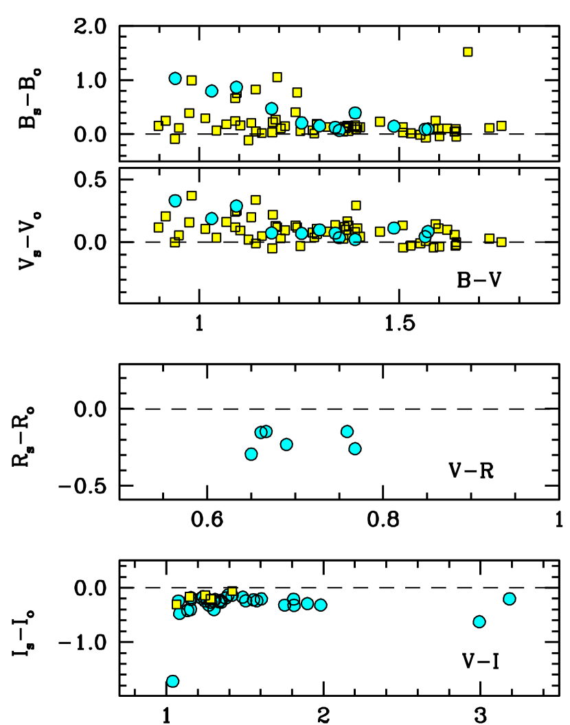
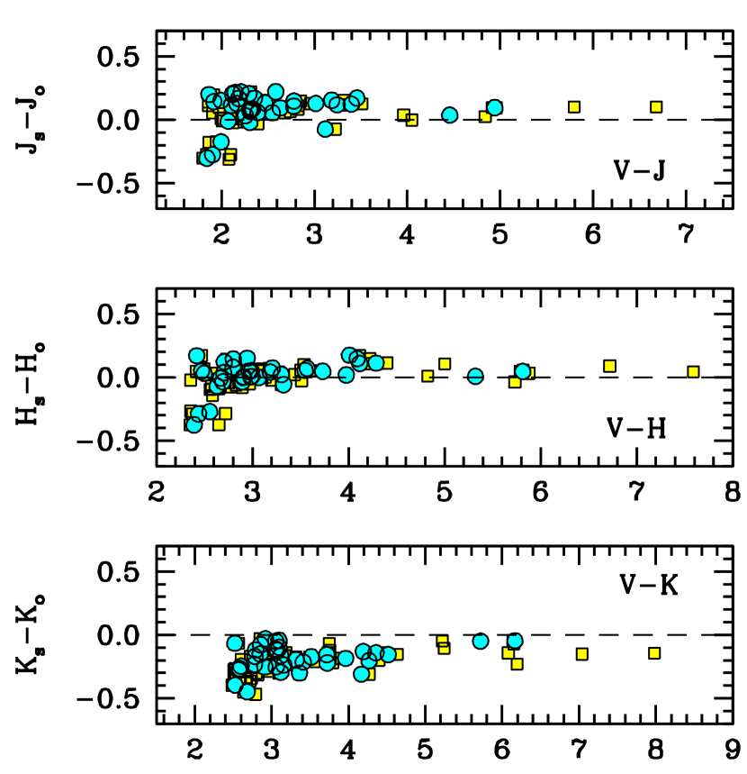
Figure 2: The $B,V,R_{c},I_{c},J,H,K$ magnitude residuals between synthetic and observed magnitudes (in the sense “syn” - “obs”) for the 94 stars in our sample.plotted vs. literature colors, according to the data of Table 1 to 5. Synthetic magnitudes derived from the numerical integration of the observed SED with the Johnson-Cousins filters. All the available photometry has been accounted for. Some stars with multiple $V$ datasets appear therefore twice in the plots and are singled out by dot and square markers, respectively.

3.2 Photometry and spectral “fine tuning”

The relevant database of broad-band photometry available in the literature for all stars in our sample can be usefully accounted for our analysis as a supplementary tool to tackle the inherent difficulty in reproducing the overall shape of stellar SED at the required accuracy level over the entire range of our observations.

As summarized in Tables 1 to 5, a wide collection of photometric catalogs can be considered, providing multicolor photometry along the range spanned by LRS and NICS spectra. Facing the observed values, one can similarly derive a corresponding set of multicolor synthetic magnitudes relying on the assembled SED of each star. Operationally, from our $f(\lambda)$ values we need to numerically assess the quantity

$$m_{\rm syn}^{j}=-2.5\,\log{{\int f(\lambda)S(\lambda)^{j}\,d\lambda}\over{\int S(\lambda)^{j}\,d\lambda}}-2.5\,\log f_{o}^{j}$$ (3)

being $m_{\rm syn}^{j}$ the synthetic magnitude in the “j-th” photometric band, identified by a filter response $S(\lambda)^{j}$ and a calibrating zero-point flux $f_{o}^{j}$. For our calculations we relied on the Buzzoni (2005) reference data (see Table 1 therein).

A comparison of our output with the available photometry is displayed in Fig. 2. The magnitude difference (in the sense “synthetic” - “observed”), is plotted in the different panels of the figure vs. observed color, according to the different photometric catalogs quoted in Tables 1 to 5. As typically two sources for $V$ magnitudes are available for most clusters, observed colors have been computed for each available $V$ dataset and are displayed with a different marker (either dot or square) in the plots.

Just a glance to Fig. 2 makes evident that systematic offsets are present between observed photometry and synthetic magnitudes. This may partly be due to zero-point uncertainty in computing eq. (3), as well as to residual systematic drifts inherent to our spectral flux calibration. In addition, from the figure one has also to report a few outliers in every band, and a notably skewed distribution of $B$ residuals. To recover for this systematics we devised an iterative $3\sigma$ clipping procedure on the data of Fig. 2 to reject deviant stars and lead synthetic magnitudes to match the standard photometric system of the observed catalogs. Our results are displayed in graphical form in the plots of Fig. 3.

After just a few rejections, our procedure quickly converged to mean magnitude offsets ($\langle{\rm Obs}-{\rm Syn}\rangle$, see Table 7) to correct eq. (3) output. After correction for this systematics, our final synthetic photometry of cluster stars (not accouting for Galactic reddening) is collected in Tables 8 and 9. According to Table 7, note that a $\sigma=0.095$ mag in total magnitude residuals evidently implies an internal accuracy in our spectral flux calibration of target stars better than 10%.

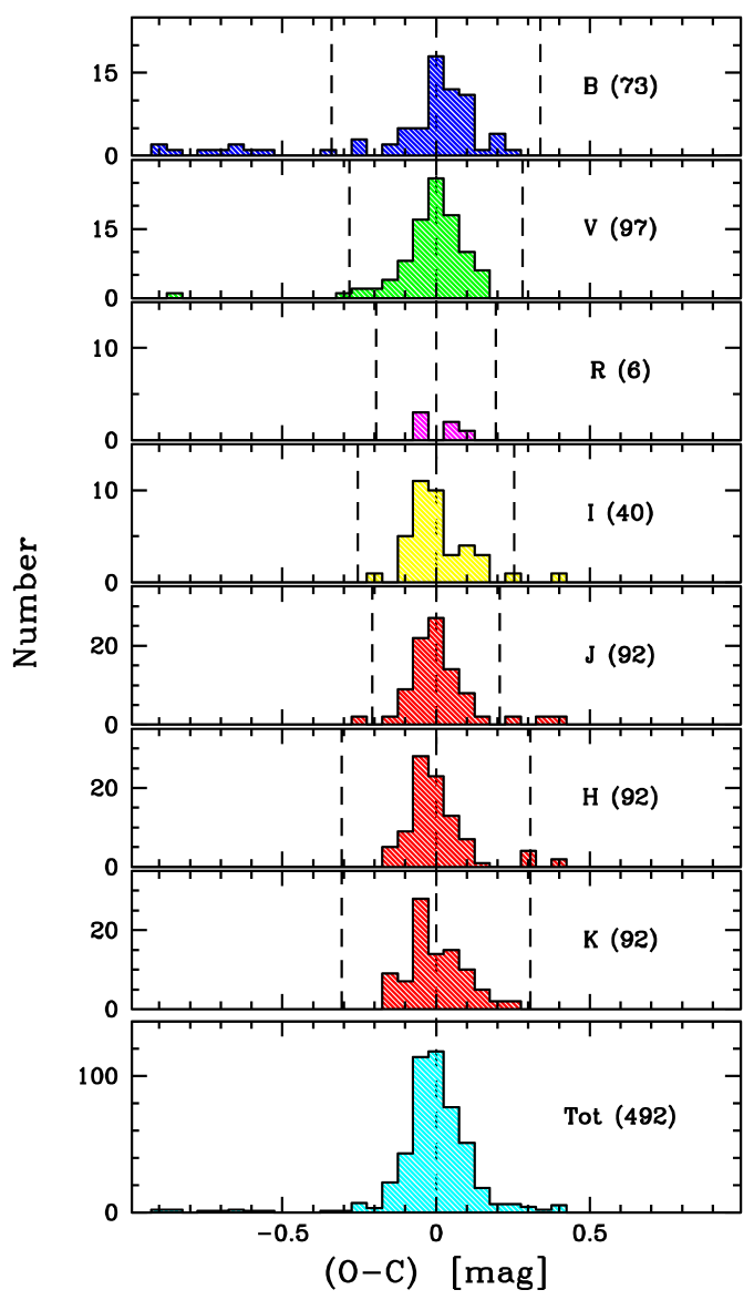
Figure 3: The histogram of magnitude residuals for the data of Fig. 2, after correction for the systematic offsets, according to Table 7. A total of 492 measures have been accounted for, as labelled in the global histogram of the bottom panel, including multiple photometry sources in the literature from Tables 1 to 5. Dashed vertical lines mark the $\pm 3\sigma$ clipping edges, according to our iterative procedure, as devised in Sec. 3.2. Mag residuals are in the sense “obs” – “syn”. After outliers rejections, the global sample of 458 measurements has, on average, $\sigma(\Delta{\rm mag})=\pm 0.095$ (see Table 7).

Table 7: Magnitude residuals between observed and theoretical magnitudes^(a)

	All the clusters
Band	$\langle Obs-Syn\rangle$	$\sigma$	Nin	Nout
B	-0.137	0.113	63	10
V	-0.091	0.094	72	1
Rc	+0.205	0.065	6	-
Ic	+0.244	0.085	38	2
J	-0.093	0.069	88	9
H	-0.012	0.102	94	3
K	+0.197	0.102	97	-
total	0.000(b)	0.095	458	25

(a) Mag residuals are in the sense of observed – synthetic one
(b) Weigthing with the number of entries, $N_{\rm in}$.

Table 8: Standard synthetic photometry from SED of target stars in globular clusters M 71, M 15, and M 2^(a)

M 15
ID	B	V	Rc	Ic	J	H	K
21300002+1209182	15.11	14.30	13.81	13.27	12.58	12.08	11.95
21295705+1208531	14.30	13.35	12.79	12.18	11.41	10.82	10.74
21295532+1210327	15.34	14.43	13.85	13.24	12.50	11.94	11.72
21300090+1208571	14.04	12.90	12.21	11.47	10.51	9.82	9.50
21295473+1208592	14.89	13.80	13.19	12.55	11.62	11.02	10.95
21300461+1210327	15.01	13.85	13.24	12.62	11.86	11.16	10.98
21295560+1212422	14.59	13.46	12.86	12.23	11.41	10.79	10.55
21300514+1210041	15.20	14.31	13.79	13.23	12.45	11.89	11.64
21295836+1209020	14.80	13.83	13.27	12.65	11.81	11.22	11.01
21295618+1210179	14.02	12.89	12.19	11.48	10.49	9.82	9.55
21295739+1209056	14.89	13.83	13.22	12.58	11.65	11.05	11.03
21300097+1210375	14.91	13.85	13.24	12.63	11.85	11.19	11.14
21300431+1210561	14.76	13.59	12.91	12.25	11.40	10.81	10.65
21301049+1210061	14.45	13.36	12.73	12.09	11.25	10.60	10.35
21300739+1210330	15.22	14.05	13.36	12.67	11.86	11.24	11.10
21300569+1210156	15.02	14.11	13.56	12.97	12.21	11.61	11.50
21300553+1208553	15.82	14.84	14.26	13.61	12.50	11.86	11.65
21295756+1209438	13.80	12.45	11.72	11.01	10.10	9.47	9.32
21295082+1211301	14.61	13.52	12.91	12.27	11.40	10.82	10.66
21295881+1209285(b)	14.62	13.40	12.70	12.03	11.17	10.57	10.42
21295716+1209175	13.96	13.03	12.45	11.84	10.98	10.36	10.20
M 2
ID	B	V	Rc	Ic	J	H	K
21333827-0054569	13.71	12.72	12.17	11.58	10.55	9.85	9.73
21333095-0052154	14.74	13.68	13.11	12.53	11.59	10.96	10.87
21332468-0044252	15.71	14.65	14.07	13.48	12.59	12.01	11.94
21331771-0047273	14.30	13.02	12.32	11.66	10.69	9.94	9.91
21331723-0048171	15.06	13.66	12.91	12.21	11.18	10.44	10.32
21331790-0048198	15.87	14.74	14.17	13.54	12.00	11.05	10.90
21331854-0051563	14.88	13.89	13.32	12.72	11.80	11.17	11.06
21331948-0051034	15.11	14.12	13.55	12.93	12.01	11.38	11.17
21331923-0049058	16.49	15.21	14.58	13.91	12.52	11.67	11.46
21332588-0046004	15.42	14.44	13.89	13.33	12.40	11.78	11.59
21333668-0051058	14.35	13.12	12.47	11.81	10.76	10.05	9.92
21333520-0046089	14.58	13.36	12.70	12.04	11.02	10.34	10.23
21333488-0047572	14.98	13.67	12.98	12.30	11.33	10.64	10.42
21333593-0049224	15.31	13.93	13.18	12.48	11.49	10.82	10.60
21333432-0051285	14.89	13.72	13.09	12.45	11.50	10.87	10.77
21332531-0052511	15.26	14.11	13.51	12.90	11.98	11.38	11.18
21333109-0054522	15.98	14.57	13.80	13.08	12.15	11.56	11.37
21333507-0051097	15.94	14.78	14.14	13.52	12.63	12.07	12.02
M 71
ID	B	V	Rc	Ic	J	H	K
19535325+1846471	14.02	12.37	11.42	10.43	8.92	8.36	7.93
19534750+1846169	14.48	13.11	12.36	11.59	10.41	9.71	9.57
19535150+1848059	13.99	12.32	11.34	10.38	9.10	8.30	8.02
19535064+1849075	14.46	13.02	12.22	11.42	10.27	9.49	9.25
19534575+1847547	14.21	12.48	11.45	10.43	9.12	8.30	8.02
19534827+1848021	14.04	12.36	11.40	10.47	9.24	8.41	8.09
19534656+1847441	14.85	13.63	12.93	12.21	11.22	10.56	10.47
19535369+1846039	15.50	14.54	14.01	13.40	12.56	12.02	11.85
19534905+1846003	14.73	13.45	12.75	12.01	10.91	10.26	10.15
19534916+1846512	14.87	13.65	13.01	12.30	11.19	10.46	10.30
19534178+1848384	15.77	14.55	13.87	13.17	12.24	11.58	11.40
19535676+1845399	15.66	14.50	13.86	13.18	12.22	11.58	11.43
19533962+1848569	15.74	14.70	14.13	13.50	12.50	11.87	11.74
19533864+1847554	15.39	14.10	13.42	12.72	11.72	11.19	11.09
19534615+1847261	14.68	13.21	12.38	11.55	10.35	9.60	9.44
19535610+1847167(c)	14.96	13.27	11.21	9.26	7.89	7.08	6.83
19534941+1844269(d)	13.88	12.02	10.71	9.42	7.96	7.20	6.96

(a) After correction for the systematic offsets, according to Table 7
(b) Dropped: I outlier
(c) Dropped: SR variable Z Sge; B, V outlier;
(d) Var AN 48.1928 (Baade, 1928)

Table 9: Standard synthetic photometry from SED of target stars in open clusters NGC 188 and NGC 6791^(a)

NGC 188
ID	B	V	Rc	Ic	J	H	K
00445253+8514055	13.65	12.34	11.66	11.01	10.04	9.41	9.45
00475922+8511322	13.68	12.13	11.38	10.73	9.78	9.20	9.25
00465966+8513157	13.87	12.40	11.71	11.11	10.25	9.71	9.67
00453697+8515084(b)	15.49	13.90	13.10	12.40	11.44	10.87	10.77
00442946+8515093(c)	15.84	14.28	13.44	12.73	11.81	11.27	11.32
00473222+8511024(d)	15.79	14.24	13.40	12.73	11.87	11.40	11.49
00554526+8512209	12.25	10.82	10.06	9.34	8.31	7.59	7.54
00463920+8523336	12.89	11.56	10.87	10.21	9.19	8.53	8.50
00472975+8524140	14.05	12.91	12.33	11.74	10.70	10.11	9.98
00441241+8509312	12.81	11.28	10.45	9.68	8.60	7.85	7.78
00432696+8509175	14.17	13.14	12.61	12.08	11.25	10.76	10.59
00471847+8519456(e)	14.89	13.03	12.19	11.47	10.54	9.99	10.07
00461981+8520086(f)	14.58	12.50	11.60	10.88	9.98	9.43	9.40
00463004+8511518(g)	15.67	14.20	13.45	12.78	11.91	11.42	11.38
00490560+8526077	13.89	12.65	12.02	11.41	10.48	9.90	9.97
00420323+8520492	11.29	9.75	8.91	8.14	7.05	6.43	6.20
NGC 6791
ID	B	V	Rc	Ic	J	H	K
19210807+3747494	15.29	13.98	13.33	12.70	11.66	11.06	10.87
19204971+3743426(h)	15.52	13.97	12.31	10.61	9.04	8.20	7.97
19205259+3744281	15.69	14.10	13.19	12.32	11.17	10.45	10.20
19205580+3742307	16.23	14.90	14.23	13.59	12.61	12.03	11.96
19205671+3743074	15.97	14.64	13.96	13.31	12.32	11.74	11.66
19210112+3742134	15.94	14.48	13.68	12.92	11.82	11.06	10.96
19211606+3746462	15.29	13.74	12.11	10.45	8.91	8.10	7.84
19213656+3740376	15.58	14.07	13.24	12.46	11.40	10.72	10.50
19210326+3741190	15.72	14.39	13.69	13.01	12.03	11.44	11.36
19213635+3739445	16.10	14.76	14.11	13.49	12.47	11.78	11.58
19212437+3735402	15.83	14.46	13.79	13.15	12.14	11.45	11.30
19212674+3735186	15.33	13.98	13.25	12.56	11.59	10.99	10.79
19211632+3752154	15.22	13.98	13.32	12.67	11.71	11.12	10.93
19211176+3752459	15.65	14.38	13.73	13.11	12.13	11.47	11.41
19202345+3754578	14.57	12.80	11.43	9.63	7.96	7.08	6.84
19205149+3739334	13.26	11.66	10.23	8.75	7.35	6.58	6.23
19203285+3753488	14.97	13.39	11.67	10.00	8.46	7.55	7.19
19200641+3744452	14.67	13.34	12.61	11.89	10.79	10.06	9.87
19200882+3744317	15.17	13.62	11.61	9.67	7.92	7.07	6.72
19203219+3744208(i)	16.22	14.77	12.46	10.23	8.18	7.29	6.93

(a) After correction for the systematic offsets, according to Table 7
(b) Dropped: B, J outlier;
(c) Dropped: B, J, H outlier;
(d) Dropped: B, J outlier;
(e) Dropped: B, J outlier;
(f) Dropped: B, J, H outlier;
(g) Dropped: B, J outlier;
(h) Dropped: I outlier; V13 - Var? (de Marchi et al., 2007)
(i) V70 $\equiv$ SBG 2240: Irr var (Mochejska, Stanek, & Kaluzny, 2003)

3.3 Stellar outliers

It could be interesting to analyze in some detail the deviant stars in our $\Delta m$ clipping procedure in order to collect further clues about their nature. Apart from the obvious impact of photometric errors, $3\sigma$ outliers may in fact more likely be displaying signs of an intrinsic physical variability in their luminosity.

As summarized in Table 10, in total 10 stars have been found to significantly ($>3\sigma$) deviate from the literature compilations. A careful check of their identifications on the Simbad database indicates that at least 3 of them are known variable (typically semir-regulars or irregulars, as expected for their nature of late-type red giants). No firm conclusions can be drawn, on the contrary, for the other seven cases, although it is evident even from a color check (see Fig. 4) that they have been picked up in an intrinsically different status with respect to previous data in the literature. We therefore commend the stars in the list of Table 10 as special candidates for further in-depth investigations for variability.

4 Spectral energy distribution and bolometric luminosity

The synthetic photometric catalogs obtained from the observed spectral database had a twofold aim: firstly, this procedure allowed us to self-consistently match broad-band magnitudes with the inferred measure of $m_{\rm bol}$, in order to obtain the corresponding value of the bolometric correction; secondly, the study of the magnitude residuals with respect to the literature data provided us with the appropriate offsets in flux rescaling such as to “smoothly” connect our optical and infrared spectra and lead therefore to a more accurate estimate of $m_{\rm bol}$.

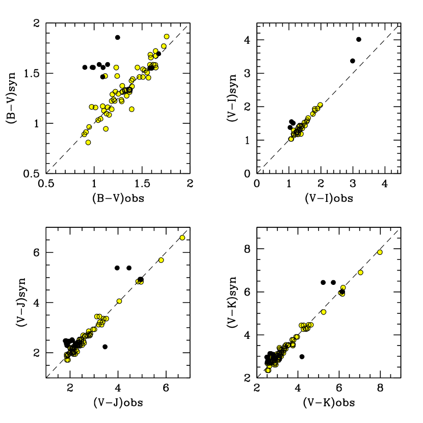
Figure 4: Color distribution of photometric outliers, according to our 3$\sigma$ clipping procedure (see Fig. 3). Target location for the whole star sample in the synthetic vs. observed color planes are displayed, with dark solid dots marking the “dropped” objects (see Table 10).

Table 10: Stellar outliers of our sample in the different photometric bands

Cluster	ID	Outlier in							Notes
		B	V	Rc	Ic	J	H	K
M15	180	…	…	…	x	…	…	…	…
M71	4212	x	x	…	…	…	…	…	Z Sge - SRa P$\sim 175^{d}$
	5755	…	…	…	x	…	…	…	V2 $\equiv$ AN 48.1928 - Ir
N188	567	x	…	…	…	x	…	…	…
	652	x	…	…	…	x	x	…	…
	1109	x	…	…	…	x	…	…	…
	630	x	…	…	…	x	…	…	…
	174	x	…	…	…	x	x	…	…
	1352	x	…	…	…	x	…	…	…
N6791	3502	…	…	…	x	…	…	…	V13 - Var?
Tot		7	1	0	3	6	2	0

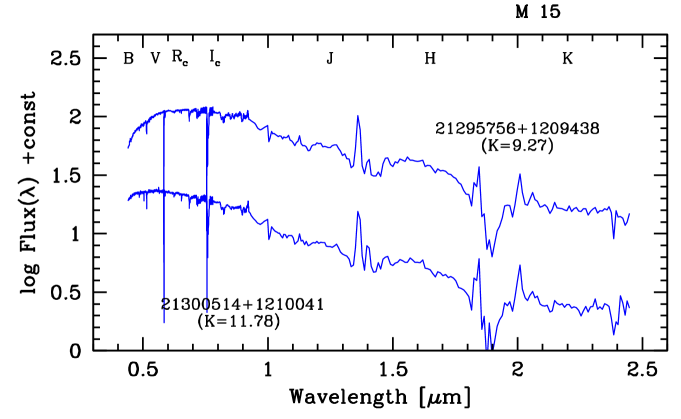
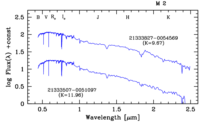
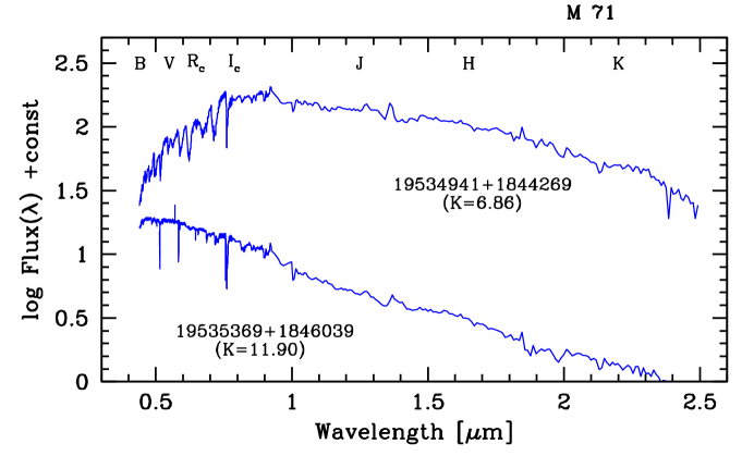
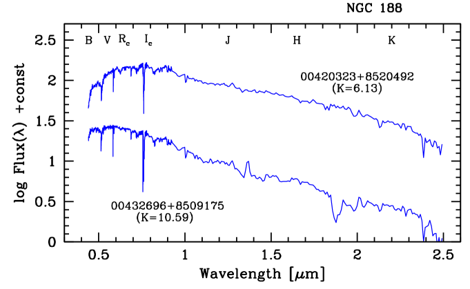
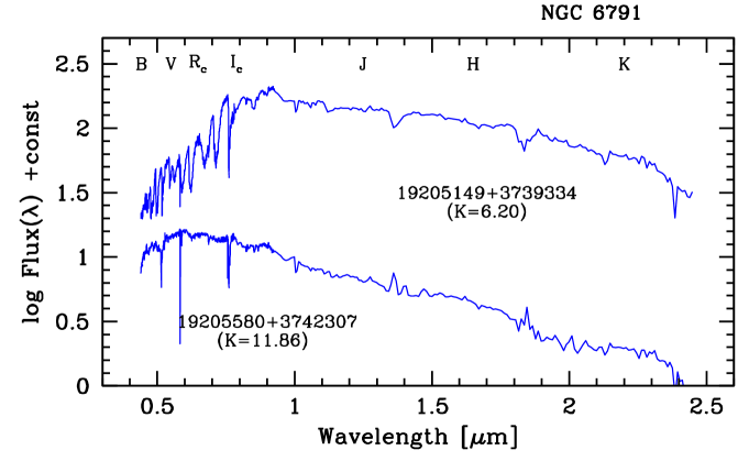
Figure 5: The resulting (dereddened) SED according to optical and infrared observations for an illustrative stellar subset of each cluster, including the brightest (and roughly coolest) and faintest (i.e. warmest) stars. Note, especially for the M 15 stars, the strong impact of telluric water vapor bands at 1.38 and 1.88 $\mu$m. Their variability along the observing nights prevented, in some cases, any accurate cleaning procedure. See discussion in Sec. 3.1.

Operationally, for the latter task, we proceeded as follows. Taking into account the individual set of $\langle Obs-Syn\rangle$ magnitude residuals, for each star in our sample we computed a mean optical and infrared offset ($\Delta m_{\rm LRS}$ and $\Delta m_{\rm NICS}$, respectively) by separately averaging the $B,V,R_{c},I_{c}$ and $J,H,K$ mag residuals. The LRS spectra and the NICS observations have then been matched by multiplying visual and IR fluxes by a factor $10^{-0.4\,(\Delta m_{\rm LRS})}$ and $10^{-0.4\,(\Delta m_{\rm NICS})}$, respectively . Foreground reddening has been corrected relying on the standard relation $k(\lambda)=A(\lambda)/E(B-V)$ (Scheffler, 2006), where the appropriate value of the color excess $E(B-V)$ is from the headers of Tables 1 to 5. In its final form, the SED is reshaped such as $f_{o}(\lambda)=f(\lambda)\,10^{0.4\,k(\lambda)E(B-V)}$.

The LRS and NICS spectra have been connected at 8800 Å, by smoothing the wavelength region between 7800 and 10000 Å (in order to gain S/N, especially for LRS poor signal at the long wavelenegth edge). In Fig. 5, we summarize our results for an illustrative set of SEDs by picking up for each cluster the brightest (i.e. roughly the coolest) and faintest (i.e. warmest) stars in our sample. Note, from the figure, the stricking presence of the CO bump about 1.6 $\mu$m (Frogel et al., 1978; Lançon & Mouhcine, 2002), as well as the broad H₂O absorption bands to which the sharper (and variable) emission of telluric water vapor superposes (see, in particular, the case of M15 stars in the figure). This made far more difficult any accurate cleaning procedure, as we discussed in Sec. 3.1.

4.1 Temperature scale

Although sampled over a wide wavelength range, SED of our stars still lacks the contribution of ultraviolet and far-infrared luminosity. Clearly, a safe assessment of this contribution is mandatory to lead to a confident measure of the bolometric magnitude. As the amount of energy released outside the spectral window of our observations critically depends on stellar temperature, our task to compute $BC$ requires in fact a parallel calibration of $T_{\rm eff}$ in the range of our red giant stars.

Among the many outstanding efforts in this direction, we have to recall the works of Flower (1975), Bessell (1979), Blackwell, Petford, & Shallis (1980), Ridgway et al. (1980), Bessell, Castelli, & Plez (1998), Houdashelt, Bell, & Sweigart (2000), VandenBerg & Clem (2003), Bertone et al. (2004) and Worthey & Lee (2006). In their exhaustive analysis, Alonso, Arribas, & Martínez-Roger (1999) provided an accurate analytical set of fitting functions, that calibrate stellar effective temperature vs. Johnson/Cousins broad-band colors. The Alonso, Arribas, & Martínez-Roger (1999) calibration relies on the IRFM estimate of stellar surface brightness, and considers stars of spectral type K5 or earlier, spanning a wide metallicity range ($-3.0\la[Fe/H]\la+0.2$). Within this range, the Authors claim an internal accuracy in the definition of $T_{\rm eff}$ better than 5%. As a further important result of their work, some colors, like $(V-I)$, $(V-L^{\prime})$, $(J-K)$ and $(I-K)$ are found to be fair tracers of temperature, almost independently from stellar metallicity.

The Alonso, Arribas, & Martínez-Roger (1999) calibration, however, strictly applies only to stars warmer than $\sim 4000$ K, while our stellar sample definitely spans a wider color range. This is certainly the case, for instance, of the brightest giant stars in NGC 6791, too (infra)red to match the Alonso et al. fitting functions. For these cases one could rely on the wider validity range of the $(B-V)$ calibration, although the advantage may only be a nominal one as any optical color, like $(B-V)$ tends naturally to saturate when moving to $T_{\rm eff}\la 4000$ K (Johnson, 1966, see also Fig. 2 in Alonso, Arribas, & Martínez-Roger, 1999).

Considering the whole set of the Alonso et al. fitting functions, we eventually chose four reference colors to assess the value of effective temperature for our stars. Two colors, namely $(B-V)$ and $(J-K)$ are entirely comprised within the LRS and NICS spectral branches, respectively, and they can therefore ostensibly probe the shape of SED in a more self-consistent way. To these two colors we also added $(V-I_{c})$ and $(V-K)$, as they provided a check of our flux calibration bridging the optical and infrared regions of the spectra.

Table 11: Inferred temperatures, bolometric magnitude and bolometric corrections for target stars in globular clusters M 71, M 15, and M 2

M 15
ID	(B-V)o	(V-Ic)o	(V-K)o	(J-K)o	TBV	TVI	TVK	TJK		$\langle$T$\rangle$	Bolo	BCV	BCK
					oK	oK	oK	oK		oK
21300002+1209182	0.71	0.87	2.08	0.58	5043	5039	5019	4748		4962	13.742	–0.25	1.83
21295705+1208531	0.85	1.01	2.34	0.62	4721	4711	4723	4619		4694	12.697	–0.34	1.99
21295532+1210327	0.81	1.03	2.44	0.73	4777	4669	4618	4307		4593	13.754	–0.37	2.07
21300090+1208571	1.04	1.27	3.13	0.96	4474	4242	4117	3806		4160	11.918	–0.67	2.45
21295473+1208592	0.99	1.09	2.58	0.62	4536	4549	4506	4619		4552	13.032	–0.46	2.12
21300461+1210327	1.06	1.07	2.60	0.83	4449	4588	4490	4068		4399	13.148	–0.39	2.20
21295560+1212422	1.03	1.07	2.64	0.81	4486	4588	4457	4113		4411	12.733	–0.42	2.22
21300514+1210041	0.79	0.92	2.40	0.76	4827	4915	4660	4231		4658	13.674	–0.33	2.07
21295836+1209020	0.87	1.02	2.55	0.75	4694	4690	4532	4256		4543	13.102	–0.42	2.13
21295618+1210179	1.03	1.25	3.07	0.89	4486	4272	4153	3941		4213	11.934	–0.65	2.42
21295739+1209056	0.96	1.09	2.53	0.57	4574	4549	4549	4782		4614	13.068	–0.45	2.07
21300097+1210375	0.96	1.06	2.44	0.66	4574	4608	4618	4499		4575	13.135	–0.41	2.03
21300431+1210561	1.07	1.18	2.67	0.70	4437	4386	4433	4387		4411	12.798	–0.48	2.18
21301049+1210061	0.99	1.11	2.74	0.85	4536	4511	4378	4024		4362	12.586	–0.46	2.27
21300739+1210330	1.07	1.22	2.68	0.71	4437	4320	4425	4360		4386	13.252	–0.49	2.19
21300569+1210156	0.81	0.98	2.34	0.66	4777	4776	4723	4499		4694	13.472	–0.33	2.01
21300553+1208553	0.88	1.07	2.92	0.80	4680	4588	4249	4136		4413	14.012	–0.52	2.40
21295756+1209438	1.25	1.28	2.86	0.73	4230	4227	4291	4307		4264	11.556	–0.58	2.27
21295082+1211301	0.99	1.09	2.59	0.69	4536	4549	4498	4414		4499	12.778	–0.43	2.15
21295716+1209175	0.83	1.03	2.56	0.73	4749	4669	4523	4307		4562	12.303	–0.42	2.14
M 2
ID	(B-V)o	(V-Ic)o	(V-K)o	(J-K)o	TBV	TVI	TVK	TJK		$\langle$T$\rangle$	Bolo	BCV	BCK
					oK	oK	oK	oK		oK
21333827-0054569	0.93	1.04	2.83	0.79	4640	4639	4312	4157		4437	11.990	–0.54	2.28
21333095-0052154	1.00	1.05	2.65	0.69	4540	4618	4447	4412		4504	13.025	–0.47	2.18
21332468-0044252	1.00	1.07	2.55	0.62	4540	4579	4530	4617		4566	14.030	–0.43	2.11
21331771-0047273	1.23	1.26	2.95	0.75	4251	4250	4230	4254		4246	12.190	–0.64	2.30
21331723-0048171	1.34	1.35	3.18	0.83	4110	4122	4090	4066		4097	12.721	–0.75	2.42
21331790-0048198	1.07	1.10	3.68	1.07		4521	3912	3618		4017	13.584	–0.97	2.71
21331854-0051563	0.93	1.07	2.67	0.71	4640	4579	4431	4358		4502	13.231	–0.47	2.19
21331948-0051034	0.93	1.09	2.79	0.81	4640	4540	4340	4111		4408	13.428	–0.51	2.28
21331923-0049058	1.22	1.20	3.59	1.03		4345	3950	3682		3992	14.083	–0.94	2.64
21332588-0046004	0.92	1.01	2.69	0.78	4655	4701	4416	4181		4488	13.814	–0.44	2.25
21333668-0051058	1.17	1.21	3.04	0.81	4314	4328	4173	4111		4232	12.271	–0.66	2.37
21333520-0046089	1.16	1.22	2.97	0.76	4326	4312	4217	4229		4271	12.528	–0.65	2.32
21333488-0047572	1.25	1.27	3.09	0.88	4215	4235	4143	3959		4138	12.813	–0.67	2.41
21333593-0049224	1.32	1.35	3.17	0.86	4133	4122	4096	4001		4088	13.002	–0.74	2.42
21333432-0051285	1.11	1.17	2.79	0.70	4391	4395	4340	4384		4378	12.980	–0.55	2.23
21332531-0052511	1.09	1.11	2.77	0.77	4417	4502	4355	4205		4370	13.414	–0.51	2.26
21333109-0054522	1.35	1.39	3.04	0.75	4098	4070	4173	4254		4149	13.675	–0.71	2.33
21333507-0051097	1.10	1.16	2.60	0.58	4404	4412	4488	4746		4512	14.102	–0.49	2.10
M 71
ID	(B-V)o	(V-Ic)o	(V-K)o	(J-K)o	TBV	TVI	TVK	TJK		$\langle$T$\rangle$	Bolo	BCV	BCK
					oK	oK	oK	oK		oK
19535325+1846471	1.39	1.54	3.75	0.86		3908	3881	3999		3929	10.455	–1.14	2.61
19534750+1846169	1.11	1.12	2.85	0.71	4466	4496	4307	4355		4406	11.760	–0.57	2.28
19535150+1848059	1.41	1.54	3.61	0.95		3908	3938	3821		3889	10.522	–1.02	2.59
19535064+1849075	1.18	1.20	3.08	0.89	4361	4356	4160	3937		4204	11.577	–0.67	2.42
19534575+1847547	1.47	1.65	3.77	0.97			3873	3784		3828	10.554	–1.15	2.62
19534827+1848021	1.42	1.49	3.58	1.02		3961	3951	3697		3870	10.606	–0.98	2.60
19534656+1847441	0.96	1.02	2.47	0.62	4710	4694	4600	4614		4654	12.438	–0.42	2.06
19535369+1846039	0.70	0.74	2.00	0.58	5289	5410	5096	4742		5134	13.556	–0.21	1.79
19534905+1846003	1.02	1.04	2.61	0.63	4609	4653	4486	4583		4583	12.209	–0.47	2.15
19534916+1846512	0.96	0.95	2.66	0.76	4710	4849	4447	4227		4558	12.434	–0.44	2.22
19534178+1848384	0.96	0.98	2.46	0.71	4710	4781	4610	4355		4614	13.405	–0.37	2.09
19535676+1845399	0.90	0.92	2.38	0.66	4815	4920	4688	4494		4729	13.379	–0.35	2.04
19533962+1848569	0.78	0.80	2.27	0.63	5082	5234	4800	4583		4925	13.636	–0.29	1.98
19533864+1847554	1.03	0.98	2.32	0.50	4593	4781	4748	5029		4788	12.980	–0.34	1.98
19534615+1847261	1.21	1.26	3.08	0.78	4318	4260	4160	4178		4229	11.728	–0.71	2.38
19534941+1844269	1.60	2.20	4.37	0.87			3676	3978		3827	9.541	–1.70	2.67

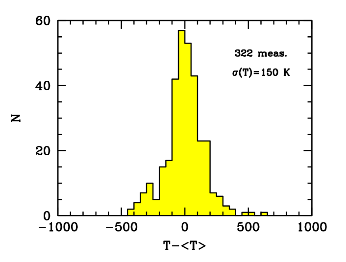
Figure 6: Histogram of temperature difference for all the data reported in Tables 8 and 9 (cols. 6 to 9) with respect to the adopted mean estimate ($\langle T\rangle$ of col. 10). A total of 322 entries are available for the whole stellar sample. The resulting distribution gives a direct measure of the internal uncertainty of our temperature scale, amounting of $\sigma(T_{\rm eff})=\pm 150$ K for the standard individual estimate.

Table 12: Inferred temperatures, bolometric magnitude and bolometric corrections for target stars in open clusters NGC 188 and NGC 6791

NGC 188
ID	(B-V)o	(V-Ic)o	(V-K)o	(J-K)o	TBV	TVI	TVK	TJK		$\langle$T$\rangle$	Bolo	BCV	BCK
					oK	oK	oK	oK		oK
00445253+851405	1.22	1.20	2.66	0.55	4398	4354	4470	4854		4519	11.552	–0.53	2.13
00475922+851132	1.46	1.27	2.65	0.49	4040	4243	4478	5078		4460	11.311	–0.56	2.09
00465966+851315	1.38	1.16	2.50	0.54	4153	4422	4602	4889		4516	11.701	–0.44	2.06
00554526+851220	1.34	1.35	3.05	0.73	4211	4129	4201	4309		4212	9.842	–0.72	2.33
00463920+852333	1.24	1.22	2.83	0.65	4366	4321	4344	4530		4390	10.706	–0.60	2.23
00472975+852414	1.05	1.04	2.70	0.68	4695	4650	4439	4444		4557	12.166	–0.49	2.21
00441241+850931	1.44	1.47	3.27	0.78	4068	3981	4078	4184		4078	10.165	–0.86	2.41
00432696+850917	0.94	0.93	2.32	0.62	4909	4893	4772	4621		4799	12.578	–0.31	2.02
00490560+852607	1.15	1.11	2.45	0.47	4516	4513	4646	5159		4708	11.945	–0.45	2.00
00420323+852049	1.45	1.48	3.32	0.81	4054	3970	4052	4114		4048	8.628	–0.87	2.46
NGC 6791
ID	(B-V)o	(V-Ic)o	(V-K)o	(J-K)o	TBV	TVI	TVK	TJK		$\langle$T$\rangle$	Bolo	BCV	BCK
					oK	oK	oK	oK		oK
19210807+3747494	1.19	1.09	2.79	0.73	4554	4544	4397	4304		4450	13.100	–0.52	2.27
19205259+3744281	1.47	1.59	3.58	0.91		3844	3953	3898		3898	12.720	–1.02	2.56
19205580+3742307	1.21	1.12	2.62	0.59	4518	4488	4527	4712		4561	14.053	–0.48	2.13
19205671+3743074	1.21	1.14	2.66	0.60	4518	4451	4495	4679		4536	13.773	–0.50	2.15
19210112+3742134	1.34	1.37	3.20	0.80	4294	4098	4138	4133		4166	13.322	–0.80	2.40
19211606+3746462	1.43	3.10	5.58	1.01			3418	3715		3566	10.646	–2.73	2.85
19213656+3740376	1.39	1.42	3.25	0.84	4214	4035	4111	4043		4101	12.902	–0.81	2.44
19210326+3741190	1.21	1.19	2.71	0.61	4518	4365	4456	4647		4496	13.493	–0.53	2.17
19213635+3739445	1.22	1.08	2.86	0.83	4499	4563	4348	4065		4369	13.867	–0.53	2.33
19212437+3735402	1.25	1.12	2.84	0.78	4446	4488	4361	4180		4369	13.561	–0.54	2.30
19212674+3735186	1.23	1.23	2.87	0.73	4482	4299	4341	4279		4350	13.034	–0.58	2.29
19211632+3752154	1.12	1.12	2.73	0.72	4686	4488	4441	4330		4486	13.119	–0.50	2.23
19211176+3752459	1.15	1.08	2.65	0.66	4629	4563	4503	4496		4548	13.538	–0.48	2.17
19202345+3754578	1.65	2.98	5.64	1.06			3407	3633		3520	9.718	–2.72	2.92
19205149+3739334	1.48	2.72	5.11	1.06			3504	3633		3568	9.043	–2.25	2.85
19203285+3753488	1.46	3.20	5.88	1.21			3368	3416		3392	10.107	–2.92	2.96
19200641+3744452	1.21	1.26	3.15	0.86	4518	4253	4166	4000		4234	12.259	–0.72	2.43
19200882+3744317	1.43	3.76	6.58	1.14			3260	3512		3386	9.664	–3.59	2.99
19203219+3744208	1.33	4.35	7.52	1.19			3120	3443		3282	9.934	–4.47	3.05

Dereddened colors for each stars in our sample provided eventually a set of nominal values of $T_{\rm eff}$, by entering the appropriate fitting functions. The “allowed” values of $T_{\rm eff}$ (i.e. if comprised within the boundary limits of the adopted calibration functions) were then averaged, deriving the mean fiducial value of the effective temperature, reported in Table 11 and 12 (column 10). In case of just one $T_{\rm eff}$ estimate (typically from $(J-K)$ color) we also added the $(V-K)$ output (reported in italics in the tables) trusting on a fairly smooth trend of the Alonso, Arribas, & Martínez-Roger (1999) calibration for this color, when extrapolated to cooler temperatures (see Fig. 8 and Fig. 10 therein).

Once combining the different temperature estimates from the four reference colors in our analysis, we report in Fig. 6 the resulting $T-\langle T\rangle$ distribution, considering the whole set of 322 individual residuals. The figure confirms that an unbiased estimate of $T_{\rm eff}$ may eventually be achieved with our procedure, within a $\pm 150$ K uncertainty on the standard measure. As, typically 2-4 useful temperature estimates are available from the colors of each star (see, again, Table 11 and 12), we may expect final $T_{\rm eff}$ values for our sample to be assessed within a 70-100 K (i.e. 1-3%) internal uncertainty.

4.2 Toward m_bol

The fiducial effective temperature, as reported in col. 10 of Table 11 and 12, provided the reference quantity to constrain the unsampled fraction of stellar luminosity, outside the wavelength limits of our spectral observations. No univocal procedure can be devised to effectively tackle this problem; from one hand, in fact, both the ultraviolet and mid- and far-infrared stellar emission can in principle be modulated by a number of different mechanisms (mass loss and stellar winds, or circumstellar gas and dust lanes thermalizing ultraviolet and optical photons, photospheric spots, pulsating variability etc.). On the other hand, one would better like to proceed with a straight heuristic approach, such as to self-consistently size up the amount of “overflown” luminosity and decide the accuracy level in its correction procedure, according to an “ex-post” analysis of the results.

On this line, we therefore decided to proceed in the most straightforward way for each star, by extrapolating its observed SED to both ultraviolet and infrared windows by means of two black-body branches, of appropriate (fixed) temperature $\langle$T$\rangle$ as in Tables 11 and 12. The two spectral branches have been separately rescaled to the (dereddened) flux values of the observed SED by setting the boundary wavelengths respectively at 4000 and 22500 Å; the integrated luminosity has then been computed within the three relevant regions of each stellar SED, identifying the ultraviolet contribution $l_{\rm UV}$ (between $0\leq\lambda\leq 4000$ Å) an optical/mid-infrared luminosity $l_{\rm obs}$ ($4000\leq\lambda\leq 22500$ Å) and a far-infrared contribution $l_{\rm FIR}$ (longward of 2.25 $\mu$m). For comparison, the same excercise has been repeated for a straight black-body spectral distribution exploring the luminosity fraction emitted shortward of $\lambda\leq 4000$ Å and longward of $\lambda\geq 22500$ Å along the temperature range of our sample.

Our results are summarized in Fig. 7. Compared to the black-body aproximation, real stars are brighter at longer wavelength and slightly fainter, on the contrary, at UV wavelength. In total, one sees from Fig. 7 that the fraction of “lost” luminosity, namely $F_{l}=(l_{\rm bol}-l_{\rm obs})/l_{\rm bol}$, turns to be about 15% for the bulk of red giants in our sample; this figure can however quickly raise with decreasing temperature, and about 1/3 of bolometric luminosity might in fact be “stored” at FIR wavelengths. Within these limits, and accounting for the 70-100 K internal uncertainty of our temperature scale, one sees from the Fig. 7 that $m_{\rm bol}$ can be secured for our sample stars within a few 0.01 mag uncertainty.

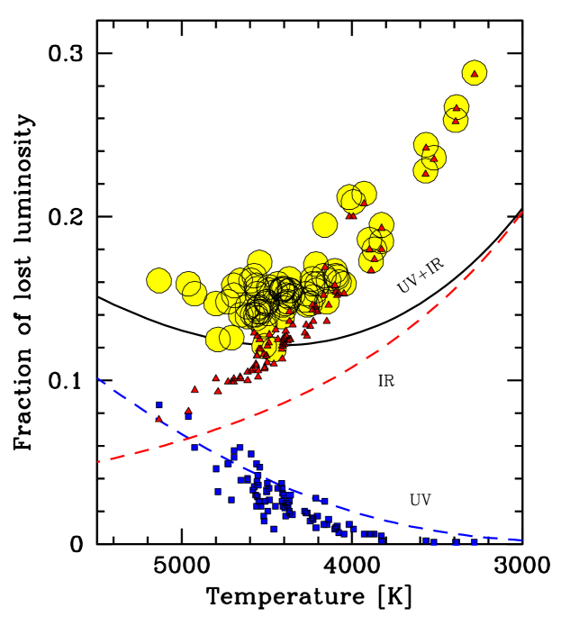
Figure 7: Estimated fraction of unsampled stellar luminosity for the stars in our sample (big solid dots). The relative contribution to stellar bolometric luminosity from lost emission at short (i.e. for $\lambda\leq 4000$ Å, small square markers on the plot) and long (i.e. for $\lambda\geq 2.25\mu$m, small triangles) wavelength is sized up by extrapolating the observed SED with two black-body (BB) “wings” at fixed $\langle$T$\rangle$, as from col. 10 of Table 11 and 12. The same excercise is carried out for a full BB spectrum along the 5500-3000 K temperature range (dashed lines labelled “UV” and “IR” for the short and long wavelength contribution, respectively, together with their summed contribution, as in the solid line). Compared to a plain BB case, note that real stars at cool temperatures display a brighter IR luminosity.

Starting from the bolometric flux (which also includes the unsampled luminosity fraction, according to our procedure), the apparent magnitude for each star derives as m${}_{\rm bol}=-2.5\,\log f_{\rm bol}+{\rm Z.P.}$. If we assume for the Sun an absolute M${}_{\rm bol}=+4.72$, and $L_{\odot}=3.89\,10^{33}$ erg s^-1, the bolometric zero point directly derives as Z.P. $=-11.50$ mag. On the same line, the BC scale is fixed once adopting an observed value for the apparent $V$ magnitude of the Sun. Following Lang (1991), if $m_{\rm V}^{\odot}=-26.78$, then M${}_{\rm V}^{\odot}=+4.79$ and a $BC_{\rm V}^{\odot}=-0.07$ mag derives. Our output, for the whole stellar sample, is reported in col. 11 of Table 11 and 12, together with the relevant (dereddened) BC to the $V$ and $K$ photometric bands (BC_V and BC_K, respectively in col. 12 and 13 of the tables).

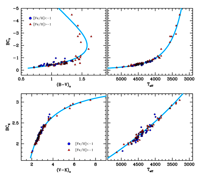
Figure 8: The BC vs. color (left panels) and BC vs. T_eff (right panels) distribution of our stellar sample (dots and triangles, for metal-poor and metal-rich stars, respectively). Synthetic colors have been corrected for Galactic reddening. Solid lines are our derived calibrations, according to the set of eqs. (4) and (5).

5 Results and discussion

The data of Tables 11 and 12 are the main output of our analysis. According to our results, we can explore three relevant relationships, linking BC with the effective temperature of stars and with two reference colors like $(B-V)$ and $(V-K)$. Given the temperature range of red giants, it could be of special relevance to consider the $K$-band BC; however, for its more general interest, we will also include in our discussion the more standard case of the BC_V.

5.1 BC-color-temperature relations

Like for a color-color diagram, the BC vs. color relationship can be regarded as an intrinsic (i.e. distance-independent) feature characterizing the stellar SED. On the corresponding theoretical side, we want also to study here the resulting dependence of BC on stellar effective temperature, a relation that allows us to more directly match the observations with the theoretical predictions of stellar model atmospheres.

In a first set of plots (see Fig. 8), we display the observed distribution of our stars in the different planes. In order to single out any possible dependence on chemical composition of stars, we marked differently metal-poor ($[Fe/H]<-1.0$ dex, dots) and metal-rich ($[Fe/H]>-1.0$ dex, triangles) objects. For better convenience in our study, we also fitted the overall distribution analytically; a useful set of fitting functions for the BC vs. T_eff relations along the $3300\lesssim T_{\rm eff}\lesssim 5000$ K temperature range results:

$$\left\{\begin{array}[]{ll}{\rm BC}_{\rm V}=-{\rm exp}(27500/{\rm T}_{\rm eff})/1000&\\ \hfill(\sigma_{\rm BC},\rho)&=(0.11,0.989)\\ \\ {\rm BC}_{\rm K}=-6.75\log({\rm T}_{\rm eff}/9500)&\\ \hfill(\sigma_{\rm BC},\rho)&=(0.05,0.978).\end{array}\right.$$ (4)

As for the color relations, the non-monotonic trend of BC_V vs. $(B-V)$ (see left upper panel in Fig. 8) prevents us to use the color as independent (i.e. “input”) variable in our fit. In this case we had therefore to adjust an inverse relation, assuming BC as the running variable. The corresponding set of analytical solutions, along the same temperature range of the previous equation set, eventually results:

$$\left\{\begin{array}[]{ll}{\rm B-V}=1.906\,\left[{\rm BC}_{\rm V}^{2}\,{\rm exp}({\rm BC}_{\rm V})\right]^{0.3}&\\ \hfill(\sigma_{\rm BV},\rho)&=(0.11,0.863)\\ \\ {\rm V-K}=1/(1-0.283~{}{\rm BC}_{\rm K})&\\ \hfill(\sigma_{\rm VK},\rho)&=(0.13,0.991),\end{array}\right.$$ (5)

All these fits are superposed to the data of Fig. 8 as a solid line.

Just on the basis of our data note how difficult it is to firmly constrain the $(B-V)$ vs. BC_V behaviour at very low temperature. From one hand, in fact, the intervening effect of the TiO absoprtion at visual wavelength (Kučinskas et al., 2005) makes the $(B-V)$ color of stars cooler than $\sim 3700$ K to strongly saturate reaching a maximum of about $(B-V)_{\rm max}\simeq 1.5$ and turning back to bluer values for later M-type stars. On the other hand, the apparent trend of our sample in this range is evidently biased by the NGC 6791 stellar population with just a few super metal rich giants constraining the BC_V trend at the most extreme negative values.

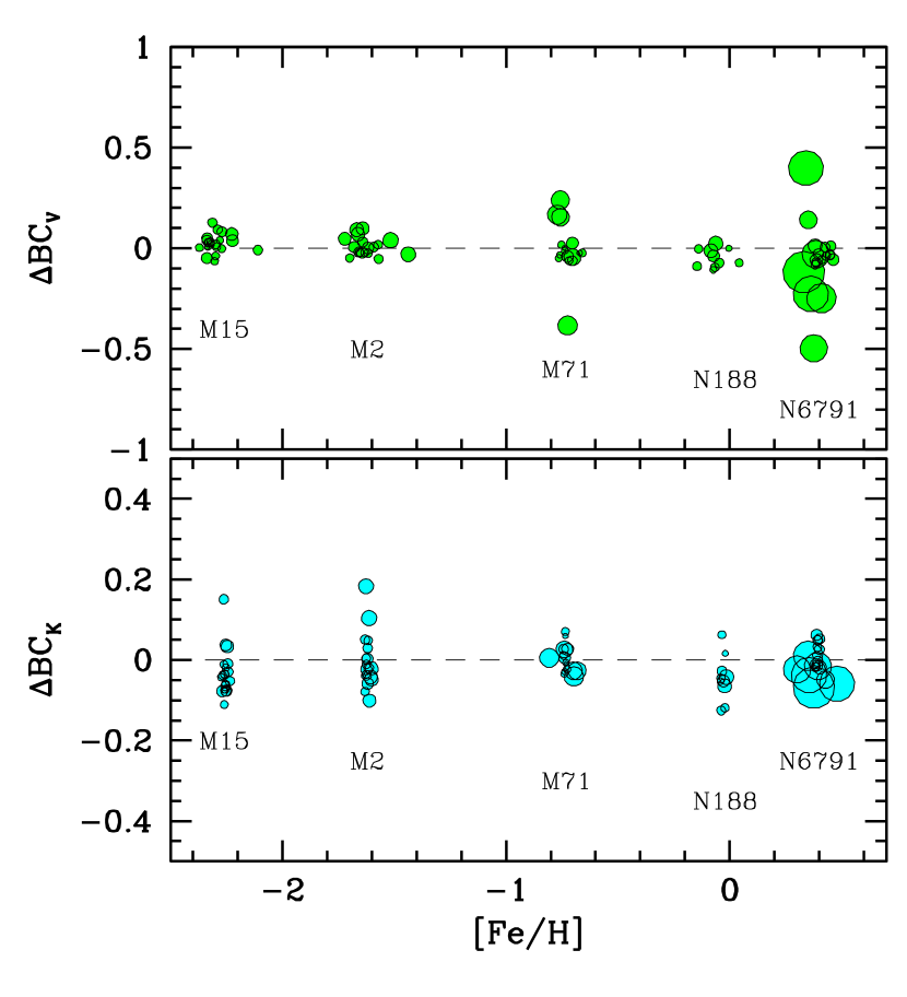
Figure 9: The distribution of BC residuals for our stellar sample vs. cluster metallicity. The displayed $\Delta$BC is intended as the difference between the values of cols. 12 and 13 of Tables 11 and 12 and the output of eq. (4) entering with the adopted effective temperature of stars, as in col. 10 of the tables. Note the lack of any evident correlation with [Fe/H], as discussed in more detail in Sec. 5.2. Data in the plot have been slightly spread around the cluster [Fe/H] value for better reading. Dot size is inversely proportional to star temperature (i.e. bigger dots = cooler red giants).

5.2 BC response to metallicity

As a part of our observing strategy, the sampled stellar population of the five clusters would in principle allow to better single out any possible dependence of BC on stellar chemical composition. As far as Helium content is concerned, for instance, this problem has already been tackled by Girardi et al. (2007) through a series of theoretical models based on the Kurucz (1992) Atlas9 model atmospheres. As a main result of their discussion, these authors did not find any relevant impact on stellar BC to optical photometric bands when Helium changes up to $\Delta Y=+0.2$, for fixed effective temperature. To some extent, this is a not so surprising behaviour; Helium is in fact a substantial contributor to mean particle weight of stellar plasma but a negligible contributor to chemical opacity. Accordingly, with varying $Y$ in the chemical mix, one has to expect a much more explicit impact on stellar temperature for fixed mass of stars, rather than on colors or SED for fixed effective temperature (as explored by Girardi et al., 2007 models, indeed).

The situation might in principle be different for the metals, mainly through their pervasive effect on stellar blanketing at short wavelength. In addition, metals are the basic ingredients required to produce molecules like TiO, SiH or CH, whose impact may be extremely relevant at blue and visual wavelength, when effective temperature lowers below 3500 K (Kučinskas et al., 2005; Bertone et al., 2008).

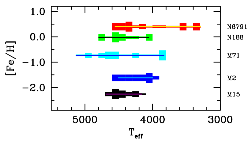
Figure 10: Temperature distribution of red-giant stars in each of the five clusters of our sample, according to Table 11 and 12. Line tickness is proportional to the star density along the spanned temperature range. Note that only cluster NGC 6791 contains stars cooler than $\sim 3800$ K.

Taking the results of Tables 11 and 12 as a reference, in Fig. 9 we plot the BC residual distribution computed as a difference between the inferred BC (cols. 12 and 13 in the tables) and the “mean” locus of eq. (4), once entering the equations with the fiducial $\langle$T$\rangle$ of col. 10. The BC residuals are displayed along the [Fe/H] distribution of the five star clusters, as labelled on the plots. Just a glance to both panels of the figure makes evident the lack of any drift of BC with stellar metallicity. Within the accuracy limits of our analysis, this means that two red giant stars of the same effective temperature but different [Fe/H] have virtually indistiguishable values of BC to $V$ and $K$ bands.

On the other hand, to correctly understand our conclusion, one has to pay attention to the different temperature regimes that mark spectral properties of red-giant stars. In fact, stars warmer than $\sim 4000$ K may have their SED depressed at short wavelength mostly in force of atomic transitions of Fe and other metals; on the contrary, for a cooler temperature, the metal opacity mainly acts in the form of molecular absorptions, making the broad band systems the prevailing features that modulate the stellar SED. As a consequence, while for stars of spectral type G or earlier any change of $Z$ simply implies a change in the blanketing strength, this may not straightforwardly be the case for later spectral types, where molecules play a much more entangled role with changing $T_{\rm eff}$.

In order to better quantify the terms of our analysis, in this respect, we display in Fig. 10 the temperature distribution of stars in our sample across the metallicity range spanned by the five clusters considered. As a stricking feature, note that only for NGC 6791 we are able to probe stars cooler than $\sim 3800$ K. The obvious caveat in our discussion is therefore that we can only assess the impact of atomic blanketing on stellar BC, while no firm conclusions can be drawn for the BC dependence on molecular absorption, facing the evident bias of our star sample against cool ($T_{\rm eff}\ll 4000$) objects.

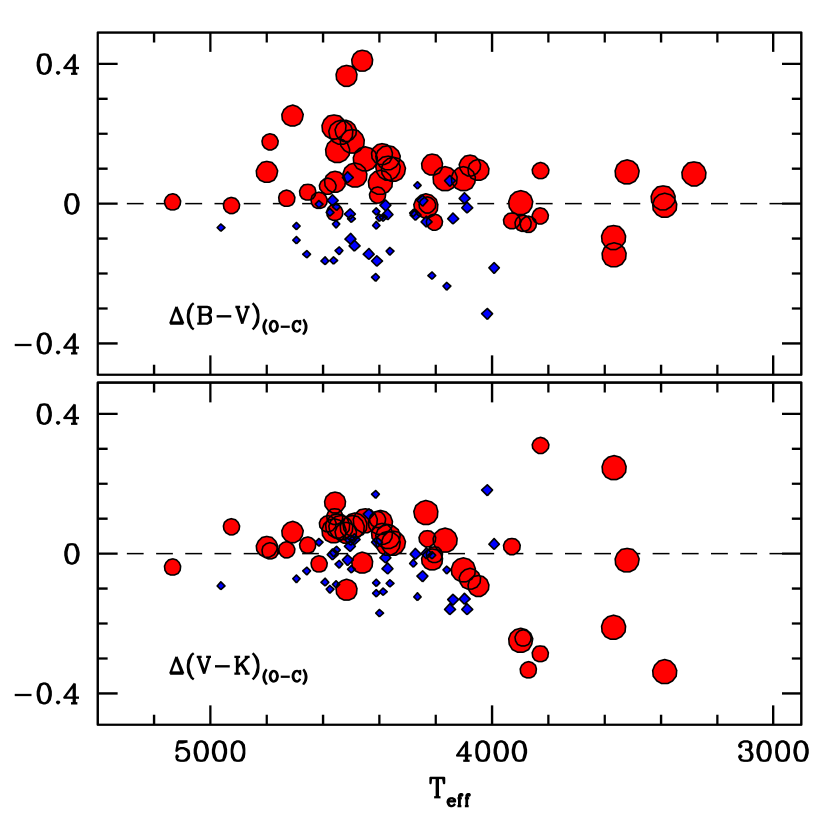
Figure 11: Residual $(B-V)$ and $(V-K)$ distribution vs. stellar temperature for stars in Table 11 and 12. Color residual is computed as a difference between observed and expected values by entering eq. (5) with the BC output of eq. (4). Metal-poor and metal-rich stars are singled out by diamonds and dot markers, respectively, taking the value $[Fe/H]=-1.0$ dex as a reference threshold. Marker size increases with [Fe/H], throughout.

As far as the blanketing is the prevailing mechanism at work in G-K stars, basic physics of stellar atmospheres leads to conclude that the $V$-band (and even more the $K$-band) luminosity are nearly unaffected by metal absorption, so that BC cannot vary much with [Fe/H]. Rather, $B$ (and even more $U$) magnitudes must be more strongly modulated by metal abundance making BC_B (and BC_U) more directly sensitive to [Fe/H]. On the other hand, as $BC_{B}=BC_{V}-(B-V)$, one can straight “translate” this metallicity effect in terms of apparent $(B-V)$ color change. This is shown in Fig. 11, where for each star in our sample we computed the residual $(B-V)$ and $(V-K)$ color as a difference between observed and expected values by entering eq. (5) with the fitted value of BC as from eq. (4). Metallicity is traced in the plot by the marker size (the bigger the marker the higher the [Fe/H] value); again, we discriminate between metal-poor (diamonds) and metal-rich (dots) stars, taking the value $[Fe/H]=-1.0$ dex as a reference threshold.

A trend of $\Delta(B-V)$ vs. cluster metallicity is now clearly evident, with the metal-poor and metal-rich star samples neatly segregated in the plot, the latter stars displaying a “redder” $(B-V)$ color (and correspondingly a positive color residual) for fixed effective temperature. On the contrary, note that both “metal-poor” and “metal-rich” stars are well mixed in the $\Delta(V-K)$ plot, witnessing once more the property of the $V-K$ color as a virtually metal-independent feature.

Considering in more detail the $\Delta(B-V)$ distribution vs. cluster metallicity, a fit to the data provides:

$$\begin{array}[]{rrlr}-\Delta BC_{B}\equiv\Delta(B-V)=&0.10&[Fe/H]&+0.13\\ &\pm 1&&\pm 2\\ \end{array}$$ (6)

with error bars at $1\sigma$ level and $({\rm rms},\rho)=(0.09\,{\rm mag},0.70)$.

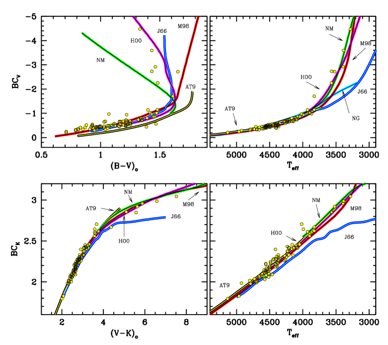
Figure 12: Same as Fig. 8, but comparing our data with different theoretical and empirical calibrations from Johnson (1966, “J66” labels), Bertone et al. (2004) using Atlas9 (Kurucz, 1992, “AT9”) and NextGen Hauschildt, Allard, & Baron (1999, “NG”) synthesis codes for model atmosphere computation, Montegriffo et al. (1998, “M98”), Houdashelt, Bell, & Sweigart (2000, “H00”) using Marcs theoretical code by (Bell & Gustafsson, 1978), and its updated version (NMarcs), as in Plez, Brett, & Nordlund (1992) and Bessell, Castelli, & Plez (1998, “NM”).

5.3 Comparison with other BC scales

For a better understanding of our results it is relevant to compare our output with other popular calibration scales often taken as a reference in the current literature and especially attempting to extend their analysis to cool (T${}_{\rm eff}\la 3500$ K) stellar temperatures. In particular, we will focus here on different theoretical BC calibrations relying on the three leading codes for advanced computation of stellar model atmospheres, namely Atlas9 (Kurucz, 1992, hereafter labelled as “AT9”), Nextgen (Hauschildt, Allard, & Baron, 1999, “NG”), both as reported by Bertone et al. (2004), and Marcs (Bell & Gustafsson, 1978, as adopted by Houdashelt et al. 2000, “H00’ label) also in its updated versions (NMarcs, as in Plez, Brett, & Nordlund (1992) and Bessell, Castelli, & Plez (1998, “NM”).

We will also consider in our analysis two empirical studies, i.e. the ones of Johnson (1966, referred to as “J66”) and Montegriffo et al. (1998, labelled as “M98”), both based on a careful analysis of infrared colors to assess the problem of the bolometric correction and a self-consistent temperature scale for red giant stars. All the bolometric scales in the figure have been shifted such as to agree with our assumption that $BC_{\rm V}^{\odot}=-0.07$ mag.

A synoptic look of the different theoretical and empirical frameworks is eased by the four panels of Fig. 12, where we report the BC_V and BC_K scales vs. observables (i.e. $(B-V)$ and $(V-K)$ colors, respectively) and theoretical (T_eff) reference quantities. In all respects, this figure is fully equivalent with, and can be compared to, Fig. 8, where we reported our own results.

Just a quick look to the different curves of Fig. 12 gives an immediate picture of the inherent uncertainties in predicted BC according to the different calibration scales. The big issue, in this regard, much deals with the way models can reproduce cool stars and observations can account for the $(B-V)$ “saturation” vs. temperature consequent to the shifted emission toward longer wavebands when stars become cooler than 3500 K. This effect makes the $B$-luminosity contribution to drop to nominal values among red giants, and the increasingly important role of molecular absorption strongly modulates optical colors of K- and M-type stars.

The still inadequate theoretical performance in modelling such cool stars with convenient accuracy fatally frustrates also any empirical effort to derive a firm temperature scale and an accurate abundance analysis for stars at the extreme edge of the temperature distribution (see, e.g., Bertone et al. 2008 and Olling et al. 2009, for useful considerations on this subject).

As far as the BC_V vs. $(B-V)$ behaviour is concerned, the reference calibrations display the largest spread, with M98 predicting increasingly redder stars with decreasing temperature. At the opposite, NM predicts a sharp color “turnback”, with BC_V increasing in absolute value among cool stars getting bluer and bluer. Definitely, the emipirical calibration by J66 still remains a reference one, fairly well tracking the observations. This trend is very closely replied also by the Marcs models by H00, that provide an even better match to the data and a substantial agreement with our fitting function as in Fig. 8.

By converting colors to the theoretical plane of effective temperature (right upper panel of Fig. 12), the picture slightly changes, in particular with a stricking discrepancy of the J66 and the theoretical NG temperature scale for T${}_{\rm eff}\la 3800$ K. Both sources predict, in fact, much shallower corrections for cool stars than we observe. An overall agreement has to be reported, on the contrary, among the other calibrations, all replying our eq. (4).

The situation is much eased in the infrared domain, where a monotonic relationship between $(V-K)$ color and BC_K characterizes red giants stars. In this new framework both the theoretical and empirical planes are well reproduced by the different calibration scales, with the only remarkable exception of J66 that, to some extent “allows” stars to store a bigger fraction of their bolometric luminosity in the infrared. This leads to a tipping BC${}_{K}\simeq 2.7$ and a too “red” $(V-K)$ for a given value of T_eff.

Combining the different pieces of information coming from these comparisons, it seems that the H00 Marcs models are by far the best ones in matching our BC estimates, closely replying in every panel of Fig. 12 our empirical fitting functions of eqs. (4), (5) and Fig. 8. In spite of this comforting appearence, however, this conclusion may be even more puzzling from a physical point of view, as the H00 models have been a fortiori tuned up such as to reproduce the observed colors of M stars. As described by the authors, this required in particular to strongly enhance the assumed TiO opacities well beyond the admitted physical range suggested by molecular theory and implemented in the “standard” Marcs library (Gustafsson et al., 2008).

6 Summary and conclusions

The firm knowledge of a fully reliable link between observations and stellar evolution models is a basic, crucial requirement for any safe use of stellar clocks and population synthesis templates in the study and interpretation of the integrated spectrophotometric properties of distant galaxies. Actually, the “stellar path” to cosmology is strictly dependent, among others, on the accurate determination of the bolometric emission of stars, with varying effective temperatures and chemical abundance.

In this framework, we have tackled the central question of the possible BC dependence on stellar metallicity by securing spectroscopic observations for a wide sample of 92 red-giant stars in five (3 globular + 2 open) Galactic clusters along the full metallicity range from $[Fe/H]=-2.2$ up to +0.4 (see Sec. 3). Spectra cover the wavelength range from 3500 Å to $2.5\mu$m, collecting optical and IR observations. A delicate task for the final settlement of our stellar database dealt with the accurate flux calibration and a consistent match of the optical and near-IR sides of the spectra such as to reproduce, for each star, the broad-band $BVR_{c}I_{c}JHK$ photometry available in the literature (Sec. 2 and 3). Allover, we are confident that stellar SED along the entire sampled wavelength range has been set up within a $\pm 10$% internal accuracy (see Table 7 and Fig. 3).

According to our previous arguments, however, one has also to carefully account for the lost contribution of ultraviolet and far-IR luminosity to the bolometric flux, depending on the effective temperature of stars. Based on the Alonso, Arribas, & Martínez-Roger (1999) T_eff-color fitting functions, we took the four colors $(B-V)$, $(J-K)$, $(V-I_{c})$, and $(V-K)$ as a reference for our calibration, leading to constrain T_eff for each stars in our sample within an estimated error better than $\pm 100$ K (see Sec. 4.1), along the whole spanned temperature range ($3300\leq T_{\rm eff}\leq 5000$ K).

The fiducial temperature allowed us to shape the unsampled portion of the SED at UV and far-IR wavelength by assuming a black-body emission independently rescaled such as to connect the short and long wavelength edge of the observed spectra. As shown in Sec. 4.2 (see also Fig. 7), under the black-body assumption, the internal uncertainty in our temperature scale only impact by a few 0.01 mag uncertainty in the inferred bolometric magnitude of our stars. In any case, by fully neglecting any unsampled spectral contribution, our data would be overestimating M_bol by at most 0.3 mag.

Making use of our new database, we have been able to draw a convenient set of fitting functions for the BC vs. T_eff, valid over the interval $3300\leq{\rm T}_{\rm eff}\leq 5000$ K (see Sec. 5.1, eq. 4). Similar relationships for BC vs. stellar colors cannot be straightforwardly derived (eq. 5), especially for the $(B-V)$, which shows a strong saturation effect for stars cooler than 3700 K, in consequence of the intervening TiO absorption at visual wavelength (Kučinskas et al., 2005). In assessing properties of such very cool stars, however, one has also to consider that our sample is strongly biased against high-metallicity values as only the red giant branch of NGC 6791 ($[Fe/H]=+0.4$) hosts stars with T${}_{\rm eff}<3700$ K.

Thanks to the wide [Fe/H] range spanned by G stars in the five clusters considered here, we explored the possible BC dependence on stellar metallicity. As far as atomic transitions prevail as the main source of metal opacity in the spectra of relatively warm (T${}_{\rm eff}\gtrsim 4000$ K) stars, our data confirm that no evident trend of BC with [Fe/H] is in place (see Fig. 9). In other words, two red giant stars of the same effective temperature but different [Fe/H] are virtually indistiguishable in the values of BC to $V$ and $K$ bands. Things may be different, however, for the $B$ (and even more for $U$) magnitudes, where the blanketing effects are more and more severe. In fact, Fig. 11 clearly shows that metal-poor stars display a “bluer” $(B-V)$ compared to corresponding metal-rich objects with the same T_eff. This leads us to conclude that a drift may be expected for $BC_{B}$ such as $BC_{B}\propto-0.10\,[Fe/H]$ among stars with fixed value of T_eff

To consistently verify our calibrations, we have shown in Fig. 12 plots of BC_V and BC_K vs. colors and T_eff, respectively, by comparing with different theoretical and empirical calibrations currently available in the literature. As far as theoretical predictions are concerned, it seems that the H00 models are the best ones matching our data in every relationship. This feature is not a surprising one, however, given the recognized intention of the H00 calculations to match M stars via “ad hoc” tuning of molecular opacity. Actually, this successful comparison may add a further piece of evidence, all the way, to the persisting limit for theory to independently assess the modelling of cool stars.

References

- Alonso, Arribas, & Martínez-Roger (1999) Alonso A., Arribas S., Martínez-Roger C., 1999, A&AS, 140, 261
- Baade (1928) Baade W., 1928, AN, 232, 65
- Bell & Gustafsson (1978) Bell R. A., Gustafsson B., 1978, A&AS, 34, 229
- Bertone et al. (2004) Bertone E., Buzzoni A., Chávez M., Rodríguez-Merino L. H., 2004, AJ, 128, 829
- Bertone et al. (2008) Bertone E., Buzzoni A., Chávez M., Rodríguez-Merino L. H., 2008, A&A, 485, 823
- Bessell (1979) Bessell M. S., 1979, PASP, 91, 589
- Bessell & Wood (1984) Bessell M. S., Wood P. R., 1984, PASP, 96, 247
- Bessell, Castelli, & Plez (1998) Bessell M. S., Castelli F., Plez B., 1998, A&A, 333, 231
- Blackwell & Lynas-Gray (1994) Blackwell D. E., Lynas-Gray A. E., 1994, A&A, 282, 899
- Blackwell, Shallis, & Selby (1979) Blackwell D. E., Shallis M. J., Selby M. J., 1979, MNRAS, 188, 847
- Blackwell, Petford, & Shallis (1980) Blackwell D. E., Petford A. D., Shallis M. J., 1980, A&A, 82, 249
- Buzzoni (1989) Buzzoni A., 1989, ApJS, 71, 817
- Buzzoni (2005) Buzzoni A., 2005, MNRAS, 361, 725
- Cassisi et al. (2004) Cassisi S., Salaris M., Castelli F., Pietrinferni A., 2004, ApJ, 616, 498
- Code et al. (1976) Code A. D., Bless R. C., Davis J., Brown R. H., 1976, ApJ, 203, 417
- Cohen, Briley, & Stetson (2005) Cohen J. G., Briley M. M., Stetson P. B., 2005, AJ, 130, 1177
- de Marchi et al. (2007) de Marchi F., et al., 2007, A&A, 471, 515
- di Benedetto & Rabbia (1987) di Benedetto G. P., Rabbia Y., 1987, A&A, 188, 114
- Dyck et al. (1996) Dyck H. M., Benson J. A., van Belle G. T., Ridgway S. T., 1996, AJ, 111, 1705
- Flower (1975) Flower P. J., 1975, A&A, 41, 391
- Flower (1977) Flower P. J., 1977, A&A, 54, 31
- Flower (1996) Flower P. J., 1996, ApJ, 469, 355
- Frogel et al. (1978) Frogel J. A., Persson S. E., Matthews K., Aaronson M., 1978, ApJ, 220, 75
- Fuensalida & Alonso (1998) Fuensalida J. J., Alonso A., 1998, NewAR, 42, 543
- Geffert & Maintz (2000) Geffert M., Maintz G., 2000, A&AS, 144, 227
- Girardi et al. (2007) Girardi L., Castelli F., Bertelli G., Nasi E., 2007, A&A, 468, 657
- González Hernández & Bonifacio (2009) González Hernández J. I., Bonifacio P., 2009, A&A, 497, 497
- Gratton et al. (1982) Gratton L., Gaudenzi S., Rossi C., Gratton R. G., 1982, MNRAS, 201, 807
- Gustafsson et al. (2008) Gustafsson B., Edvardsson B., Eriksson K., Jørgensen U. G., Nordlund Å., Plez B., 2008, A&A, 486, 951
- Hauschildt, Allard, & Baron (1999) Hauschildt P. H., Allard F., Baron E., 1999, ApJ, 512, 377
- Houdashelt, Bell, & Sweigart (2000) Houdashelt M. L., Bell R. A., Sweigart A. V., 2000, AJ, 119, 1448
- Hunt et al. (1998) Hunt L. K., Mannucci F., Testi L., Migliorini S., Stanga R. M., Baffa C., Lisi F., Vanzi L., 1998, AJ, 115, 2594
- Johnson (1966) Johnson H. L., 1966, ARA&A, 4, 193
- Kaluzny & Rucinski (1995) Kaluzny J., Rucinski S. M., 1995, A&AS, 114, 1
- Kuiper (1938) Kuiper G. P., 1938, ApJ, 88, 429
- Kučinskas et al. (2005) Kučinskas A., Hauschildt P. H., Ludwig H.-G., Brott I., Vansevičius V., Lindegren L., Tanabé T., Allard F., 2005, A&A, 442, 281
- Kurucz (1992) Kurucz R. L., 1992, IAUS, 149, 225
- Lançon & Mouhcine (2002) Lançon A., Mouhcine M., 2002, A&A, 393, 167
- Lang (1991) Lang K.R., 1991, Astrophysical Data: planets and stars (Heidelberg: Springer Verlag)
- Manduca & Bell (1979) Manduca A., Bell R. A., 1979, PASP, 91, 848
- Massey et al. (1988) Massey P., Strobel K., Barnes J. V., Anderson E., 1988, ApJ, 328, 315
- Mochejska, Stanek, & Kaluzny (2003) Mochejska B. J., Stanek K. Z., Kaluzny J., 2003, AJ, 125, 3175
- Montegriffo et al. (1998) Montegriffo P., Ferraro F. R., Origlia L., Fusi Pecci F., 1998, MNRAS, 297, 872
- Olling et al. (2009) Olling R. P., et al., 2009, Astro2010: The Astronomy and Astrophysics Decadal Survey, Science White Papers, no. 226 (see also astroph/0902.3197)
- Perrin et al. (1998) Perrin G., Coude Du Foresto V., Ridgway S. T., Mariotti J.-M., Traub W. A., Carleton N. P., Lacasse M. G., 1998, A&A, 331, 619
- Platais et al. (2003) Platais I., Kozhurina-Platais V., Mathieu R. D., Girard T. M., van Altena W. F., 2003, AJ, 126, 2922
- Plez, Brett, & Nordlund (1992) Plez B., Brett J. M., Nordlund A., 1992, A&A, 256, 551
- Ramírez & Meléndez (2005) Ramírez I., Meléndez J., 2005, ApJ, 626, 446
- Richichi et al. (1998) Richichi A., Ragland S., Stecklum B., Leinert C., 1998, A&A, 338, 527
- Ridgway et al. (1980) Ridgway S. T., Jacoby G. H., Joyce R. R., Wells D. C., 1980, AJ, 85, 1496
- Rosenberg et al. (2000) Rosenberg A., Piotto G., Saviane I., Aparicio A., 2000, A&AS, 144, 5
- Scheffler (2006) Scheffler, H., 2006, in Landolt-Börnstein - Group VI Astronomy and Astrophysics, Chap. 7 (Heidelberg: Springer Verlag), p.46
- Skrutskie et al. (2006) Skrutskie M. F., et al., 2006, AJ, 131, 1163
- Stetson, Bruntt, & Grundahl (2003) Stetson P. B., Bruntt H., Grundahl F., 2003, PASP, 115, 413
- Stetson, McClure, & VandenBerg (2004) Stetson P. B., McClure R. D., VandenBerg D. A., 2004, PASP, 116, 1012
- Tokunaga & Vacca (2005) Tokunaga A. T., Vacca W. D., 2005, PASP, 117, 421
- Tripicco & Bell (1995) Tripicco M. J., Bell R. A., 1995, AJ, 110, 3035
- VandenBerg & Clem (2003) VandenBerg D. A., Clem J. L., 2003, AJ, 126, 778
- Wesselink (1969) Wesselink A. J., 1969, MNRAS, 144, 297
- Worthey & Lee (2006) Worthey G., Lee H., 2006, astro-ph/0604590