Polarized Superfluidity in the imbalanced attractive Hubbard model

Abstract

We investigate the attractive Hubbard model in infinite spatial dimensions by means of dynamical mean-field theory. Using a continuous-time Monte Carlo algorithm in the Nambu formalism as an impurity solver, we directly deal with the superfluid phase in the population imbalanced system. By calculating the superfluid order parameter, the magnetization, and the density of states, we discuss how the polarized superfluid state is realized in the attractive Hubbard model at quarter filling. We find that a drastic change in the density of states is induced by spin imbalanced populations in the superfluid state.

1 Introduction

The superfluid state in ultracold atomic systems has attracted much interest since the successful realization of the Bose-Einstein condensation (BEC) of rubidium atoms.[1] In addition to bosonic systems, the superfluid state has been observed in two-component fermionic systems, [2] where Cooper pairs formed by the attractive interactions condense at low temperatures. Due to the high controllability of the interaction strength and the particle number, interesting phenomena have been observed such as the BCS-BEC crossover[3, 4, 5] and the superfluid state with imbalanced populations. [6, 7] These observations stimulate further experimental and theoretical investigations on fermionic systems.

In the existing literature on spin imbalanced populations various ordered ground states have been proposed to be more stable than the polarized superfluid (PSF) state, which is naively expected to be realized below the critical temperature. One interesting candidate is the Fulde-Ferrell-Larkin-Ovchinnikov (FFLO) phase,[8, 9] where Cooper pairs are formed with nonzero total momentum. This phase has been observed in the high field region in ${\rm CsCoIn_{5}},$[10, 11, 12] and has theoretically been discussed in the latter compound,[13] as well as cold atoms with imbalanced populations.[14, 15] Another proposed phase is the breached-pair (BP) phase, where both the superfluid order parameter and the magnetization are finite at zero temperature. [16, 17, 18, 19, 20] When one considers higher dimensional optical lattice systems, the BP state without momentum dependence may be one of the appropriate ground states. It has recently been clarified that the PSF state is closely connected to the BP phase at half filling in the three-dimensional Hubbard model with intermediate attractive interactions. [21] However, the Hubbard model has a high symmetry at half filling, [22, 24, 23] and the conclusions may not be applicable to an optical lattice system, where the particle density is not fixed at half filling due to the existence of the confining potential. Therefore, it is important to clarify how the PSF state and the BP state are realized in a system away from half filling.

With this purpose in mind, we investigate the attractive Hubbard model at quarter filling to discuss the effect of the imbalanced spin populations on the superfluid state. By combining dynamical mean-field theory (DMFT) [25, 26, 27, 28] with the continuous time quantum Monte Carlo (CTQMC) method,[29] we study the low temperature properties of the system quantitatively. Here, we extend the CTQMC method in the continuous-time auxiliary field (CTAUX) formulation[30] to treat the PSF state in the Nambu formalism. By calculating the order parameter of the superfluid state, the magnetization, and the density of states, we clarify the nature of the PSF state in the spin imbalanced system.

The paper is organized as follows. In §2, we introduce the model Hamiltonian for the attractive Hubbard model and briefly summarize the DMFT framework. The CTQMC algorithm in the Nambu formalism is explained in some detail in §3. In §4, we focus on the attractive Hubbard model at quarter filling to discuss how the PSF state is realized at low temperatures. A brief summary is given in §5.

2 Model and Method

We consider a correlated fermion system with attractive interactions, which may be described by the Hubbard Hamiltonian,

$$\hat{\cal{H}}=\sum_{(i,j),\sigma}\left[-t-\left(\mu+h\sigma\right)\delta_{ij}\right]c^{\dagger}_{i\sigma}c_{j\sigma}-U\sum_{i}n_{i\uparrow}n_{i\downarrow},$$ (1)

where $c_{i\sigma}$ ($c^{\dagger}_{i\sigma}$) is an annihilation (creation) operator of a fermion on the $i$th site with spin $\sigma$, and $n_{i\sigma}=c^{\dagger}_{i\sigma}c_{i\sigma}$. $U$ is the onsite attractive interaction, $t$ is the transfer integral between sites, $\mu$ is the chemical potential, and $h$ is the magnetic field. For $h=0$ the ground state properties of the model have been studied in one dimension,[31, 32, 33, 35, 34, 36] two dimensions[22, 24, 37] and infinite dimensions.[40, 41, 38, 39, 42, 23] Both the BCS-BEC crossover and the possibility of a supersolid state have been discussed. On the other hand, there are few studies addressing the effect of imbalanced populations beyond the static mean-field approach except for one dimensional system.[15]

To study the infinite dimensional attractive Hubbard model at an arbitrary filling, we make use of DMFT. [25, 26, 27, 28] In DMFT, the original lattice model is mapped to an effective impurity model, which accurately takes into account local particle correlations. The lattice Green’s function is obtained via a self-consistency condition imposed on the impurity problem. This treatment is formally exact in infinite dimensions, and the DMFT method has successfully been applied to strongly correlated fermion systems.

When the superfluid state is treated in the framework of DMFT, the local self-energy should be described by a $2\times 2$ matrix as

$$\hat{\Sigma}(i\omega_{n})=\left(\begin{array}[]{cc}\Sigma_{\uparrow}(i\omega_{n})&S(i\omega_{n})\\ S(i\omega_{n})&-\Sigma^{*}_{\downarrow}(i\omega_{n})\end{array}\right),$$ (2)

where $\Sigma_{\sigma}(i\omega_{n})\;[S(i\omega_{n})]$ is the diagonal (off-diagonal) element of the self-energy in the Nambu formalism and the Matsubara frequency is $\omega_{n}=(2n+1)\pi/\beta$, with $\beta$ the inverse temperature. Note that we do not take into account $k$-dependent correlations, but dynamical correlations through the frequency-dependent self-energy. This enables us to discuss the stability of the $s$-wave superfluid state more quantitatively beyond the static mean-field theory.

The lattice Green’s function is then given in terms of the local self-energy as,

$$\hat{G}^{-1}(k,i\omega_{n})=\left(i\omega_{n}+h\right)\hat{\sigma}_{0}+\left(\mu-\epsilon_{k}\right)\hat{\sigma}_{z}-\hat{\Sigma}\left(i\omega_{n}\right),$$ (3)

where $\hat{\sigma}_{0}$ and $\hat{\sigma}_{z}$ are the identity matrix and the $z$-component of the Pauli matrix, and $\epsilon_{k}$ is the dispersion relation for the non-interacting system. The local lattice Green’s function is obtained as,

$$\hat{G}(i\omega_{n})=\int dk\hat{G}(k,i\omega_{n}).$$ (4)

In the calculations, we use the semi-circular density of states, $\rho(x)=1/N\sum_{k}\delta(x-\epsilon_{k})=2/\pi D\sqrt{1-(x/D)^{2}}$, where $D$ is the half bandwidth. The self-consistency equation[43] is then given by

$$\hat{G}_{0,\text{imp}}^{-1}(i\omega_{n})=\left(i\omega_{n}+h\right)\hat{\sigma}_{0}+\mu\hat{\sigma}_{z}-\left(\frac{D}{4}\right)^{2}\hat{\sigma}_{z}\hat{G}(i\omega_{n})\hat{\sigma}_{z}.$$ (5)

When one discusses low energy properties in strongly correlated systems in the framework of DMFT, an impurity solver is necessary to obtain the Green’s function and the self-energy for the effective impurity model. There are various numerical techniques such as exact diagonalization[44] and the numerical renormalization group.[45, 46, 47] A recently developed and particularly powerful method is CTQMC. In this method, Monte Carlo samplings of collections of diagrams for the partition function are performed in continuous time, and thereby the Trotter error, which originates from the Suzuki-Trotter decomposition, is avoided. Furthermore, this method is applicable to more general classes of models than the Hirsch-Fye algorithm.[48] The CTQMC method has successfully been applied to various systems such as the Hubbard model,[49, 50] the periodic Anderson model, [51] the Kondo lattice model[52] and the Holstein-Hubbard model.[53]

3 Continuous-Time Quantum Monte Carlo simulations in the Nambu Formalism

In this section, we explain the CTAUX method,[30] and extend it to treat the superfluid state. A similar solver was recently proposed, [51] where the superfluid state is treated by means of a canonical transformation. The Anderson impurity model we have to solve is given by

$$H = H_{0}+H_{U},$$ (6)

$$H_{0} = \sum_{p\sigma}\epsilon_{p\sigma}n_{p\sigma}+\sum_{p\sigma}\left(V_{p\sigma}d_{\sigma}^{\dagger}a_{p\sigma}+h.c.\right)$$ (7)

$$+ \sum_{p}\left(\Delta_{p}a_{p\uparrow}^{\dagger}a_{p\downarrow}^{\dagger}+h.c.\right)+\sum_{\sigma}E_{d\sigma}n_{d\sigma},$$

$$H_{U} = -U\left[n_{d\uparrow}n_{d\downarrow}-\frac{1}{2}\left(n_{d\uparrow}+n_{d\downarrow}-1\right)\right],$$ (8)

where $a_{p\sigma}(d_{\sigma})$ annihilates a fermion with spin $\sigma$ in the $p$th orbital of the effective baths (the impurity site). $\epsilon_{p\sigma}$ and $\Delta_{p}$ represent the effective bath, and $V_{p\sigma}$ represents the hybridization between the effective bath and the impurity site. $E_{d\sigma}$ is the energy level for the impurity site, $n_{p\sigma}=a_{p\sigma}^{\dagger}a_{p\sigma}$, and $n_{d\sigma}=d_{\sigma}^{\dagger}d_{\sigma}$. We note that the total particle number is not conserved in the model. The Green’s functions should be defined by $\hat{G}(\tau)=\langle T_{\tau}\hat{\psi}(\tau)\hat{\psi}^{\dagger}(0)\rangle$, where $T_{\tau}$ is the imaginary-time ordering operator and $\hat{\psi}^{\dagger}(\tau)=(c^{\dagger}_{\uparrow}(\tau)\;c_{\downarrow}(\tau))$. The Green’s functions are $2\times 2$ matrices with elements

$$\hat{G}(\tau)=\left(\begin{array}[]{cc}G_{\uparrow}(\tau)&F(\tau)\\ F^{*}(\tau)&-G_{\downarrow}(-\tau)\end{array}\right),$$ (9)

where $G_{\sigma}(\tau)=\langle T_{\tau}c_{\sigma}(\tau)c_{\sigma}^{\dagger}(0)\rangle$ denotes the normal Green’s function, and $F(\tau)=\langle T_{\tau}c_{\uparrow}(\tau)c_{\downarrow}(0)\rangle$ and $F^{*}(\tau)=\langle T_{\tau}c^{\dagger}_{\downarrow}(\tau)c^{\dagger}_{\uparrow}(0)\rangle$ anomalous Green’s functions. Here, we have chosen the Green’s functions $G_{\sigma}(\tau)$ to be positive.

To perform simulations, we consider here a weak coupling CTQMC approach. The partition function $Z$ is given by

$$Z = {\rm Tr}\left[e^{-\beta H_{1}}T_{\tau}e^{-\int_{0}^{\beta}d\tau H_{2}(\tau)}\right]$$ (10)

$$= \sum_{n=0}^{\infty}\int_{0}^{\beta}d\tau_{1}\int_{\tau_{1}}^{\beta}d\tau_{2}\cdots\int_{\tau_{n-1}}^{\beta}d\tau_{n}$$

$$\times {\rm Tr}\Big{[}e^{-(\beta-\tau_{n})H_{1}}(-H_{2})e^{-(\tau_{n}-\tau_{n-1})H_{1}}\cdots$$

$$\cdots e^{-(\tau_{2}-\tau_{1})H_{1}}(-H_{2})e^{-\tau_{1}H_{1}}\Big{]},$$

where we have divided the impurity Hamiltonian Eq. (6) into two parts as,

$$H_{1} = H-H_{2},$$ (11)

$$H_{2} = H_{U}-K/\beta$$ (12)

$$= \frac{K}{2\beta}\sum_{s=-1,1}e^{\gamma s\left(n_{\uparrow}+n_{\downarrow}-1\right)},$$

with $\gamma=\cosh^{-1}(1+\beta U/2K)$, and $K$ some nonzero constant. The introduction of the Ising variable $s$ in $H_{2}$ enables us to perform simulations away from half-filling. An $n$th order configuration $c=\{s_{1},s_{2},\cdots,s_{n};\tau_{1},\tau_{2},\cdots,\tau_{n}\}$ corresponding to auxiliary spins $s_{1},s_{2},\ldots,s_{n}$ at imaginary times $\tau_{1}<\tau_{2}<\ldots<\tau_{n}$ contributes a weight

$$w_{c} = e^{-K}\left(\frac{Kd\tau}{2\beta}\right)^{n}e^{-\gamma\sum s_{i}}Z_{0}\;{\rm det}\;\left[\hat{N}^{(n)}\right]^{-1}$$ (13)

to the partition function. Here, $Z_{0}={\rm Tr}[e^{-\beta H_{1}}]$ and $\hat{N}^{(n)}$ is an $n\times n$ matrix, where each element consists of a $2\times 2$ matrix:

$$\left[\hat{N}^{(n)}\right]^{-1} = \hat{\Gamma}^{(n)}-\hat{g}^{(n)}\left(\hat{\Gamma}^{(n)}-\hat{I}^{(n)}\right),$$ (14)

$$\hat{I}^{(n)}_{ij} = \delta_{ij}\hat{\sigma}_{0},$$ (15)

$$\hat{\Gamma}^{(n)}_{ij} = \delta_{ij}e^{\gamma s_{i}}\hat{\sigma}_{0},$$ (16)

$$\hat{g}^{(n)}_{ij} = \left(\begin{array}[]{cc}g_{0\uparrow}(\tau_{i}-\tau_{j})&f_{0}(\tau_{i}-\tau_{j})\\ -f_{0}^{*}(\tau_{i}-\tau_{j})&g_{0\downarrow}(\tau_{j}-\tau_{i})\end{array}\right),\hskip 11.38109pt$$ (19)

with $i,j=1,2,\cdots n$.

The sampling process must satisfy ergodicity and (as a sufficient condition) detailed balance. For ergodicity, it is enough to insert or remove the Ising variables with random orientations at random times to generate all possible configurations. To satisfy the detailed balance condition, we decompose the transition probability as

$$p\left(i\rightarrow j\right)=p^{\rm prop}\left(i\rightarrow j\right)p^{\rm acc}\left(i\rightarrow j\right),$$ (20)

where $p^{\rm prop}(p^{\rm acc})$ is the probability to propose (accept) the transition from the configuration $i$ to the configuration $j$. Here, we consider the insertion and removal of the Ising spins as one step of the simulation process, which corresponds to a change of $\pm 1$ in the perturbation order. The probability of insertion/removal of an Ising spin is then given by

$$p^{\rm prop}(n\rightarrow n+1) = \frac{d\tau}{2\beta},$$ (21)

$$p^{\rm prop}(n+1\rightarrow n) = \frac{1}{n+1}.$$ (22)

For this choice, the ratio of the acceptance probabilities becomes

$$\frac{p^{\rm acc}\left(n\rightarrow n+1\right)}{p^{\rm acc}\left(n+1\rightarrow n\right)}=\frac{K}{n+1}e^{-\gamma s_{n+1}}\frac{\det N^{(n)}}{\det N^{(n+1)}}.$$ (23)

When the Metropolis algorithm is used to sample the configurations, we accept the transition from $n$ to $n\pm 1$ with the probability

$${\rm min}\left[1,\frac{p^{\rm acc}\left(n\rightarrow n\pm 1\right)}{p^{\rm acc}\left(n\pm 1\rightarrow n\right)}\right].$$ (24)

In each Monte Carlo step, we measure the following Green’s functions ($0<\tau<\beta$),

$$G_{\sigma}(\tau) = \frac{1}{Z}{\rm Tr}\left[e^{-\beta H}c_{\sigma}(\tau)c^{\dagger}_{\sigma}(0)\right],$$ (25)

$$F(\tau) = \frac{1}{Z}{\rm Tr}\left[e^{-\beta H}c_{\uparrow}(\tau)c_{\downarrow}(0)\right],$$ (26)

$$F^{*}(\tau) = \frac{1}{Z}{\rm Tr}\left[e^{-\beta H}c^{\dagger}_{\downarrow}(\tau)c^{\dagger}_{\uparrow}(0)\right].$$ (27)

By using Wick’s theorem, the contribution of a certain configuration $c$ is given by

$$G_{\sigma}^{c}(\tau) =\det[N^{(n)}]{\rm det}\left(\begin{array}[]{cc}\left[N^{(n)}\right]^{-1}&Q_{\sigma}\\ R_{\sigma}&g_{0\sigma}(\tau)\end{array}\right),$$ (30)

$$F^{c}(\tau) =\det[N^{(n)}]{\rm det}\left(\begin{array}[]{cc}\left[N^{(n)}\right]^{-1}&Q^{\prime}\\ R^{\prime}&f_{0}(\tau)\end{array}\right),$$ (33)

$$F^{*c}(\tau) =\det[N^{(n)}]{\rm det}\left(\begin{array}[]{cc}\left[N^{(n)}\right]^{-1}&Q^{*\prime}\\ R^{*\prime}&f^{*}_{0}(\tau)\end{array}\right),$$ (36)

where $Q_{\sigma},Q^{\prime},Q^{*\prime},R_{\sigma},R^{\prime},R^{*\prime}$ are vectors, in which the $i$th element ($i=1,2,\cdots,n$) is defined by

$$Q_{\uparrow i} = \{-g_{0\uparrow}(\tau_{i})\;\;f^{*}_{0}(\tau_{i})\}^{T},$$ (37)

$$Q_{\downarrow i} = \{f_{0}(\tau_{i}-\tau)\;\;g_{0\downarrow}(\tau-\tau_{i})\}^{T},$$ (38)

$$Q^{\prime}_{i} = \{-f_{0}(\tau_{i})\;\;-g_{0\downarrow}(-\tau_{i})\}^{T},$$ (39)

$$Q^{*\prime}_{i} = Q_{\uparrow i},$$ (40)

$$R_{\uparrow i} = (e^{\gamma s_{i}}-1)\{g_{0\uparrow}(\tau-\tau_{i})\;\;f_{0}(\tau-\tau_{i})\},$$ (41)

$$R_{\downarrow i} = (e^{\gamma s_{i}}-1)\{f^{*}_{0}(-\tau_{i})\;\;-g_{0\downarrow}(\tau_{i})\},$$ (42)

$$R^{\prime}_{i} = R_{\uparrow i},$$ (43)

$$R^{*\prime}_{i} = (e^{\gamma s_{i}}-1)\{f^{*}_{0}(\tau-\tau_{i})\;\;-g_{0\downarrow}(\tau_{i}-\tau)\}.\hskip 5.69054pt$$ (44)

In this paper, we use the half bandwidth $D$ as the unit of the energy and set $K=1$ in the CTQMC simulations. We thus calculate static physical quantities such as the order parameter of the superfluid state $\Delta$ and the magnetization $m$, which are defined by

$$\Delta = \langle c_{\uparrow}c_{\downarrow}\rangle=F(0_{+}),$$ (45)

$$m = \sum_{\sigma}\sigma\langle c_{\sigma}^{\dagger}c_{\sigma}\rangle=-\sum_{\sigma}\sigma G_{\sigma}(0_{+}).$$ (46)

Furthermore, by applying the maximum entropy method (MEM) to the Green’s functions, we deduce the spectral functions, which allows us to discuss static and dynamical properties of the system.

In Fig. 1, we show, as an example, the normal and anomalous Green’s functions when $U=1$, $h=0.1$ and $T=0.01$. The Green’s functions were measured on a grid of a thousand points.

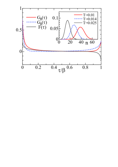
Figure 1: Green’s functions as a function of $\tau/\beta$ in the quarter-filled system at $U=1,h=0.1$ and $T=0.01$. The solid (dashed) line represents the Green’s function for the up (down) spin and the thin line the anomalous Green’s function. The inset shows the probability distribution for configurations with perturbation order $n$ at the temperatures $T=0.01,0.014$ and $0.025$.

In this case, the system has both a magnetization $m\sim 0.005$ and a superfluid order parameter $\Delta\sim 0.2$. Therefore, we can say that the PSF state is realized in this parameter region. Note that a large difference appears between $G_{\uparrow}(\tau)$ and $G_{\downarrow}(\tau)$ near $\tau\sim 0$ and $\beta$ although the magnetization is small. This may affect dynamical properties.

4 Superfluid state in a magnetic field

Here, we focus on the attractive Hubbard model at quarter filling to discuss how the PSF state is realized at low temperatures. First, we perform calculations at a fixed temperature. Results for the systems with weak (intermediate) coupling $[U=1~{}(U=2)]$ are shown in Fig. 2.

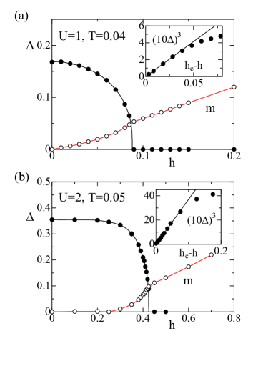
Figure 2: The superfluid order parameter and the magnetization as a function of the magnetic field when $U=1,T=0.04$ (a), and $U=2,T=0.05$ (b). The insets show the critical behavior for the order parameter.

When no magnetic field is applied, the system is in the superfluid state at low temperatures. In fact, we find that the superfluid gap opens around the Fermi level and that peak structures appear at the edges of the gap in the density of states, as shown in Fig. 3.

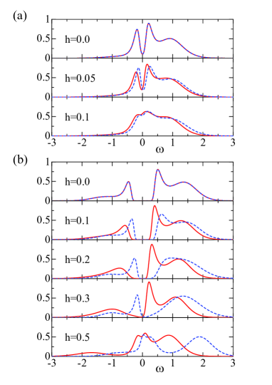
Figure 3: Solid (dashed) lines represent the spectral functions for fermions with up (down) spin when $U=1,T=0.04$ (a), and $U=2,T=0.05$ (b).

These results are consistent with those obtained by other groups.[40, 42] If a magnetic field is applied to the system, these peaks move to low (high) energy region in the density of states for up (down) spin. Pairing correlations are then suppressed, and a magnetization is induced, as shown in Fig. 2. We note that at low temperatures, the introduction of a magnetic field has little effect on the static quantities $\Delta$ and $m$, but produces a drastic change in the density of states. In fact, it is found that when $U=2$ and $h=0.3$, one of the peaks disappears and the other remains above (below) the Fermi level in the density of states for up (down) spin although the superfluid gap is still open. Therefore, we conclude that dynamical properties are strongly affected by the spin imbalanced populations. A further increase in the magnetic field smears the superfluid gap around the Fermi level and the superfluid order parameter vanishes. This suggests the existence of a phase transition to the normal metallic phase. By examining the critical behavior $\Delta\sim|h-h_{c}|^{1/\delta}$ with the exponent $\delta=3$, we obtain the critical fields $h_{c}(U=1,T=0.04)\sim 0.0885$ and $h_{c}(U=2,T=0.05)\sim 0.425$, as shown in the insets of Fig. 2. It is also found that the phase transition induces a cusp singularity in the magnetization curve. The results obtained here are in contrast to those in the half-filled attractive Hubbard model on the simple cubic lattice, where the PSF state smoothly connects to the normal metallic phase.[21] This may result from the fact that the competition between the superfluid state and the charge density wave state enhances fluctuations for the superfluid order parameter due to the high symmetry at half filling. It would be interesting to clarify this point, which is beyond the scope of our study.

We also show the temperature dependence of the superfluid order parameter in Fig. 4.

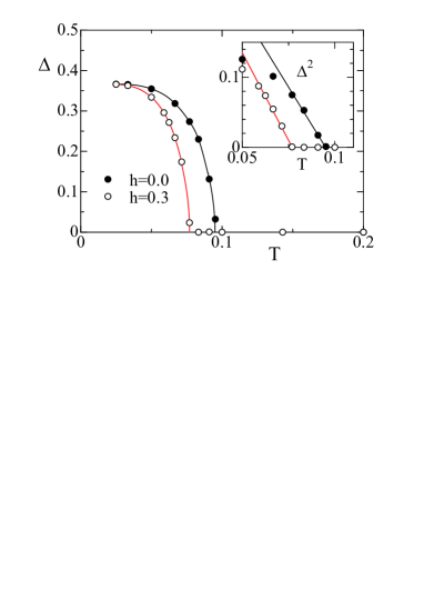
Figure 4: The order parameter for the superfluid state $\Delta$ as a function of the temperature $T$ when $U=2$.

When $h=0$, as temperature is decreased, the order parameter $\Delta$ appears where the phase transition occurs from the normal metallic state to the superfluid state. By examining the critical behavior $\Delta\sim|T-T_{c}|^{\beta}$ with the exponent $\beta=1/2$, we obtain the critical temperature $T_{c}\sim 0.095$, as shown in the inset of Fig. 4. On the other hand, when the magnetic field is switched on, pairing correlations are suppressed. For $h=0.3$, it is found that the superfluid order parameter is decreased and the critical temperature is shifted to $T_{c}\sim 0.077$. A large magnetic field destroys the superfluidity and the normal metallic state is realized instead. In fact, we could not find any finite $\Delta$ down to low temperatures ($T=0.033$) in the case $h=0.6$. Note that the two curves saturate almost at the same value of $\Delta$ when $T\rightarrow 0$. This suggests that by increasing the magnetic field at zero temperature, the superfluid ground state is little affected and eventually a first order phase transition occurs to the normal metallic state. Therefore, it may be difficult to realize the BP state with finite magnetization.

To clarify this, we next examine how the magnetization appears in the superfluid state. In Fig. 5, we show a semi-log plot of the magnetization normalized by the applied field.

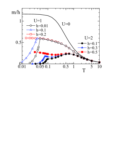
Figure 5: Normalized magnetization $m/h$ as a function of temperature $T$ in the system with $U=0,1$ and $2$.

When a tiny magnetic field is applied to the system, $m/h$ corresponds to the magnetic susceptibility $\chi$. In the noninteracting system ($U=0$), $m/h$ saturates at low temperatures at the value $\chi(T=0)=2\rho(x=0)\sim 1.16$, and in the interacting case, our results are consistent with those obtained by Keller et al.[39] Increasing the attractive interaction in the presence of a finite magnetic field, fermion pairs are formed at high temperatures and thereby magnetic correlations are suppressed and the magnetization decreases. When the magnetic field is small enough, a phase transition occurs to the superfluid state at low temperatures. In this state, the magnetization rapidly decreases below the critical temperature, as shown in Fig. 5. This means that it is difficult to realize the BP ground state with finite $\Delta$ and $m$ at zero temperature. To confirm this, we also show the quantity $\Delta_{T}(=-T\log m)$ as a function of temperature in Fig. 6.

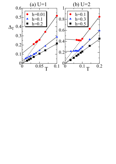
Figure 6: $\Delta_{T}(=-T\log m)$ as a function of temperature $T$ in the system with $U=1$ (a) and $U=2$ (b). Lines are guides to eyes.

When $T\rightarrow 0$, the data approach a finite value in the superfluid state, while they approach zero in the normal metallic state. This means that the magnetization decays exponentially in $1/T$ in the superfluid state. Therefore, we can say that the BP state is not realized in the ground state, at least, in this quarter-filled system.

By performing similar calculations, we have obtained the phase diagram for the spin imbalance parameter $P[=(N_{\uparrow}-N_{\downarrow})/(N_{\uparrow}+N_{\downarrow})=2m]$, which is sometimes used in the discussion of optical lattice systems, as shown in Fig. 7.

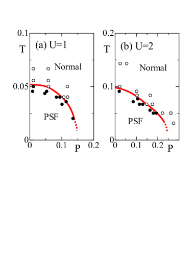
Figure 7: Phase diagrams for the quarter-filled system with $U=1$ and $U=2$. Open (solid) circles indicate the normal (PSF) state and phase boundaries are guides to eyes.

When the temperature decreases with fixed imbalanced populations, a phase transition occurs to the PSF state. Figure 8 shows the density of states for each spin component in a system with $P\sim 0.02$ and $U=2$.

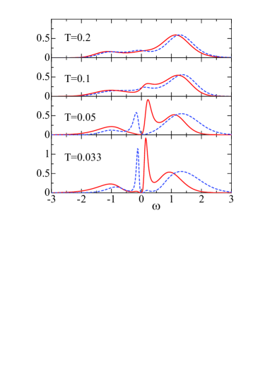
Figure 8: Density of states for the system with $U=2$ and $P=0.02$ when $T=0.2,0.1,0.05$ and $0.033$.

It is found that at high temperatures $(T>T_{c})$, the normal metallic state is realized, where the spin imbalanced populations have little effect on the density of states. By contrast, in the superfluid state $(T<T_{c})$, a large difference appears in the low energy region of the spectral functions. Since the populations with up spin are slightly larger than those with down spin in the case considered, a certain energy is necessary to add a fermion with up spin in the superfluid state. Therefore the low energy peak appears above the Fermi level in the density of states for up spin at low temperatures. As temperature is lowered to zero, it may be difficult to realize a state with $P\neq 0$, as discussed before. We cannot rule out that a phase transition from the superfluid phase back to the metallic phase (reentrant behavior) will occur at temperatures below the range accessible to us. In any event, the imbalanced populations should play a crucial role at very low temperatures, in particular, in the dynamical properties.

5 Summary

We have investigated the attractive Hubbard model in infinite dimensions by means of DMFT. Here, we have used the CTAUX method as an impurity solver, which has been extended to treat the superfluid state directly in the Nambu formalism. We have calculated the superfluid order parameter, the magnetization, and the density of states systematically to discuss how the PSF state is realized at low temperatures. It was found that when the temperature is lowered in the presence of a fixed magnetic field, a superfluid phase transition indeed occurs in our model, and the magnetization exponentially decays in the superfluid state. This suggests that the BP phase is unstable at zero temperature. We have also found that a drastic change in the density of states is induced by spin imbalanced populations in the superfluid state although the spin imbalance has little effect on static quantities. It is an interesting problem to clarify how such dynamical properties are realized in a low dimensional optical lattice with a confining potential, which is now under consideration.

References

- [1] M. H. Anderson, J. R. Ensher, M. R. Matthews, C. E. Wieman, and E. A. Cornell: Science 269 (1995) 198.
- [2] C. A. Regal, M. Greiner, and D. S. Jin: Phys. Rev. Lett. 92 (2004) 040403.
- [3] S. Jochim et al.: Science 302 (2003) 2101.
- [4] M. W. Zwierlein et al.: Phys. Rev. Lett. 91 (2003) 250401.
- [5] T. Bourdel et al.: Phys. Rev. Lett. 93 (2004) 050401.
- [6] M. W. Zwierlein, A. Schirotzek, C. H. Shunck, and W. Ketterle: Science 311 (2006) 492.
- [7] G. B. Partridge, W. Li, R. I. Kamar, Y. Liao, and R. G. Hulet: Science 311 (2006) 503.
- [8] P. Fulde and R. A. Ferrell: Phys. Rev. 135 (1964) A550.
- [9] A. I. Larkin and Y. N. Ovchinnikov: Sov. Phys. JETP 20 (1965) 762.
- [10] H. A. Radovan, N. A. Fortune, T. P. Murphy, S. T. Hannahs, E. C. Palm, S. W. Tozer, and D. Hall: Nature 425 (2003) 51.
- [11] A. Bianchi, R. Movshovich, C. Capan, P. G. Pagliuso, and J. L. Sarrao: Phys. Rev. Lett. 91 (2003) 187004.
- [12] Y. Matsuda and H. Shimahara: J. Phys. Soc. Jpn. 76 (2007) 051005
- [13] H. Adachi and R. Ikeda: Phys. Rev. B 68 (2003) 184510; K. Miyake: J. Phys. Soc. Jpn. 77 (2008) 123703; Y. Yanase and M. Sigrist: J. Phys. Soc. Jpn. 78 (2009) 114715; D. F. Agterberg, M .Sigrist, and H. Tsunetsugu: Phys. Rev. Lett. 102 (2009) 207004.
- [14] T. K. Koponen, T. Paananen, J.-P. Martikainen, and P. Törmä: Phys. Rev. Lett. 99 (2007) 120403; Y. Chen, Z. D. Wang, F. C. Zhang, and C. S. Ting: Phys. Rev. B 79 (2009) 054512; H. Tamaki, K. Miyake, and Y. Ohashi: J. Phys. Soc. Jpn. 78 (2009) 073001.
- [15] M. Tezuka and M. Ueda: Phys. Rev. Lett. 100 (2008) 110403; M. Machida, S. Yamada, M. Okumura, Y. Ohashi, and H. Matsumoto: Phys. Rev. A 77 (2008) 053614.
- [16] G. Sarma: J. Phys. Chem. Solids 24 (1963) 1029.
- [17] W. V. Liu and F. Wilczek: Phys. Rev. Lett. 90 (2003) 047002.
- [18] D. E. Sheehy and L. Radzihovsky: Phys. Rev. Lett. 96 (2006) 060401.
- [19] D. T. Son and M. A. Stephanov: Phys. Rev. A 74 (2006) 013614.
- [20] S. Pilati and S. Siorgini: Phys. Rev. Lett. 100 (2008) 030401.
- [21] T.-L. Dao, M. Ferrero, A. Georges, M. Capone, and O. Parcollet: Phys. Rev. Lett. 101 (2008) 236405.
- [22] A. Moreo and D.J. Scalapino: Phys. Rev. Lett. 66 (1991) 946.
- [23] J. K. Freericks, M. Jarrell and M. J. Scalapino: Phys. Rev. B 48 (1993) 6302.
- [24] T. Paiva, R. R. dos Santos, R. T. Scalettar, and P. J. H. Denteneer: Phys. Rev. B 69 (2004) 184501.
- [25] W. Metzner and D. Vollhardt: Phys. Rev. Lett. 62 (1989) 324.
- [26] E. Müller-Hartmann: Z. Phys. B 74 (1989) 507.
- [27] A. Georges, G. Kotliar, W. Krauth and M. J. Rozenberg: Rev. Mod. Phys. 68 (1996) 13.
- [28] T. Pruschke, M. Jarrell, and J. K. Freericks: Adv. Phys. 42 (1995) 187.
- [29] A. N. Rubtsov, V. V. Savkin and A. I. Lichtenstein: Phys. Rev. B 72 (2005) 035122.
- [30] E. Gull, P. Werner, O. Parcollet and M. Troyer: Europhys. Lett. 82 (2008) 57003.
- [31] E. H. Lieb and F. Y. Wu: Phys. Rev. Lett. 20 (1968) 1445.
- [32] H. Shiba: Prog. Theor. Phys. 48 (1972) 2171.
- [33] M. Machida, S. Yamada, Y. Ohashi, and H. Matsumoto: Phys. Rev. A 74 (2006) 053621.
- [34] F. K. Pour, M. Rigol, S. Wessel, and A. Muramatsu: Phys. Rev. B 75 (2007) 161104.
- [35] G. Xianlong, M. Rizzi, M. Polini, R. Fazio, M. P. Tosi, V. L. Campo Jr., and K. Capelle: Phys. Rev. Lett. 98 (2007) 030404.
- [36] Y. Fujihara, A. Koga, and N. Kawakami: Phys. Rev. A 79 (2009) 013610.
- [37] A. Koga, T. Higashiyama, K. Inaba, S. Suga, and N. Kawakami: J. Phys. Soc. Jpn. 77 (2008) 073602; Phys. Rev. A 79 (2009) 013607.
- [38] Y. Y. Suzuki, S. Saito, and S. Kurihara: Prog. Theor. Phys. 102 (1999) 953.
- [39] M. Keller, W. Metzner, and U. Schollwöck: Phys. Rev. Lett. 86 (2001) 4612.
- [40] A. Garg, H. R. Krishnamurthy, and M. Randeria: Phys. Rev. B 72 (2005) 024517.
- [41] A. Toschi, M. Capone, and C. Castellani: Phys. Rev. B 72 (2005) 235118.
- [42] J. Bauer, A. C. Hewson, and N. Dupuis: Phys. Rev. B 79 (2009) 214518; J. Bauer and A. C. Hewson: Europhys. Lett. 85 (2009) 27001.
- [43] A. Georges, G. Kotliar, and W. Krauth: Z. Phys. B 92 (1993) 313.
- [44] M. Caffarel and W. Krauth: Phys. Rev. Lett. 72 (1994) 1545.
- [45] H. R. Krishna-murthy, J. W. Wilkins, and K. G. Wilson: Phys. Rev. B 21 (1980) 1003.
- [46] R. Bulla, T. Costi, and Th. Pruschke: Rev. Mod. Phys. 80 (2008) 395.
- [47] O. Sakai and Y. Kuramoto: Solid State Comm. 89 (1994) 307.
- [48] J. E. Hirsch and R. M. Fye, Phys. Rev. Lett. 56, 2521 (1986).
- [49] P. Werner, A. Comanac, L. de’Medici, M. Troyer, and A. J. Millis: Phys. Rev. Lett. 97 (2006) 076405; P. Werner and A. J. Millis: Phys. Rev. B 75 (2007) 085108;
- [50] P. Werner and A. J. Millis: Phys. Rev. B 74 (2006) 155107; Phys. Rev. Lett. 99 (2007) 126405; P. Werner, E. Gull, and A. J. Millis: Phys. Rev. B 79 (2009) 115119.
- [51] D. J. Luitz and F. F. Assaad: arXiv: 0909.2656.
- [52] J. Otsuki, H. Kusunose, P. Werner, and Y. Kuramoto: J. Phys. Soc. Jpn. 76 (2007) 114707; J. Otsuki, H. Kusunose, and Y. Kuramoto: Phys. Rev. Lett. 102 (2009) 017202.
- [53] F. F. Assaad and T. C. Lang: Phys. Rev. B 76 (2007) 035116; P. Werner and A. J. Millis: Phys. Rev. Lett. 99 (2007) 146404.