Technical Report # KU-EC-13-3:
Distribution of Relative Edge Density of the Graphs Based on a Random Digraph Family

Abstract

The vertex-random graphs called proximity catch digraphs (PCDs) have been introduced recently and have applications in pattern recognition and spatial pattern analysis. A PCD is a random directed graph (i.e., digraph) which is constructed from data using the relative positions of the points from various classes. Different PCDs result from different definitions of the proximity region associated with each data point. We consider the underlying and reflexivity graphs based on a family of PCDs which is determined by a family of parameterized proximity maps called proportional-edge (PE) proximity map. The graph invariant we investigate is the relative edge density of the underlying and reflexivity graphs. We demonstrate that, properly scaled, relative edge density of these graphs is a $U$-statistic, and hence obtain the asymptotic normality of the relative edge density for data from any distribution that satisfies mild regulatory conditions. By detailed probabilistic and geometric calculations, we compute the explicit form of the asymptotic normal distribution for uniform data on a bounded region in the usual Euclidean plane. We also compare the relative edge densities of the two types of the graphs and the relative arc density of the PE-PCDs. The approach presented here is also valid for data in higher dimensions.

short title: Relative Edge Density of Graphs Based on a Digraph Family

Keywords: asymptotic normality; central limit theorem; proximity catch digraphs; random graphs and digraphs; $U$-statistic

AMS 2000 Subject Classification: 60D05; 60F05; 62E20; 05C80; 05C20; 60C05

^⋆ This research was supported by the European Commission under the Marie Curie International Outgoing Fellowship Programme via Project # 329370 titled PRinHDD.

1 Introduction

Classification and clustering have received considerable attention in the probabilistic and statistical literature. In this article, the probabilistic properties of a graph invariant of a family of random graphs is investigated. Vertex-random digraphs are directed graphs in which each vertex corresponds to a data point, and directed edges (i.e., arcs) are defined in terms of a bivariate relation on the data points. For example, nearest neighbor digraphs are defined by placing an arc between each vertex and its nearest neighbor. Priebe et al., (2001) introduced the class cover catch digraphs (CCCDs) in $\mathbb{R}$ and gave the exact and the asymptotic distribution of the domination number of the CCCDs for uniform data on bounded intervals. DeVinney et al., (2002), Marchette and Priebe, (2003), Priebe et al., 2003a , Priebe et al., 2003b , and DeVinney and Priebe, (2006) applied the concept in higher dimensions and demonstrated relatively good performance of CCCDs in classification. Their methods involve data reduction (i.e., condensing) by using approximate minimum dominating sets as prototype sets (since finding the exact minimum dominating set is an NP-hard problem in general and for CCCD in multiple dimensions (see DeVinney and Priebe, (2006)). Furthermore, the exact and the asymptotic distribution of the domination number of the CCCDs are not analytically tractable in multiple dimensions. For the domination number of CCCDs for one-dimensional data, a SLLN result is proved in DeVinney and Wierman, (2003), and this result is extended by Wierman and Xiang, (2008); furthermore, a generalized SLLN result is provided by Wierman and Xiang, (2008), and a CLT is also proved by Xiang and Wierman, (2009). The asymptotic distribution of the domination number of CCCDs for non-uniform data in $\mathbb{R}$ is also calculated in a rather general setting (Ceyhan, (2008)).

Ceyhan, (2005) generalized CCCDs to what is called proximity catch digraphs (PCDs). Let $(\Omega,\mathcal{M})$ be a measurable space and $\mathcal{X}_{n}=\{X_{1},X_{2},\ldots,X_{n}\}$ and $\mathcal{Y}_{m}=\{Y_{1},Y_{2},\ldots,Y_{m}\}$ be two sets of $\Omega$-valued random variables from classes $\mathcal{X}$ and $\mathcal{Y}$, respectively, with joint probability distribution $F_{X,Y}$. A PCD is comprised of a set of vertices and a set of arcs. For example, in the two class case, with classes $\mathcal{X}$ and $\mathcal{Y}$, the $\mathcal{X}$ points are the vertices and there is an arc from $x_{1}\in\mathcal{X}_{n}$ to $x_{2}\in\mathcal{X}_{n}$, based on a binary relation which measures the relative allocation of $x_{1}$ and $x_{2}$ with respect to $\mathcal{Y}$ points. The PCDs are closely related to the class cover problem of Cannon and Cowen, (2000). The class cover problem for a target class, say $\mathcal{X}$, refers to finding a collection of neighborhoods, $N_{i}$ around $X_{i}$ such that (i) $\mathcal{X}_{n}\subseteq\bigl{(}\bigcup_{i}N_{i}\bigr{)}$ and (ii) $\mathcal{Y}_{m}\cap\bigl{(}\bigcup_{i}N_{i}\bigr{)}=\emptyset$. A collection of neighborhoods satisfying both conditions is called a class cover. A cover satisfying (i) is a proper cover of class $\mathcal{X}$ while a cover satisfying (ii) is a pure cover relative to class $\mathcal{Y}$. See Priebe et al., (2001) and Cannon and Cowen, (2000) for more detail on the class cover problem. The first PCD family is introduced by Ceyhan and Priebe, (2003); the parameterized version of this PCD is developed by Ceyhan et al., (2007) where the relative arc density of the PCD is calculated and used for spatial pattern analysis. Ceyhan and Priebe, (2005) introduced another digraph family called proportional edge PCDs (PE-PCDs) and calculated the asymptotic distribution of its domination number and used it for the same purpose (Ceyhan and Priebe, (2007); Ceyhan, (2011)). The relative arc density of this PCD family is also computed and used in spatial pattern analysis (Ceyhan et al., (2006)).

The graphs based on digraphs are obtained by replacing arcs in the digraph by edges based on bivariate relations. If symmetric arcs are replaced by edges, then we obtain the reflexivity graph; and if all arcs are replaced by edges disallowing multi-edges, then we obtain the underlying graph (Chartrand et al., (2010)). Properly scaled, we demonstrate that the relative edge density of the underlying and reflexivity graphs of PE-PCDs is a $U$-statistic, which has asymptotic normality by the general central limit theory of $U$-statistics. Furthermore, we derive the explicit form of the parameters of the asymptotic normal distribution of the relative edge density of the PCDs based on uniform data in a bounded region in the Euclidean plane.

For the digraphs introduced by Priebe et al., (2001) (i.e., CCCDs), whose relative arc density is also of the $U$-statistic form, the asymptotic mean and variance of the relative density is not analytically tractable, due to geometric difficulties encountered. However, for the PCDs introduced in Ceyhan et al., (2006), and Ceyhan et al., (2007), the relative arc density has tractable asymptotic mean and variance. The same holds for the underlying graphs as well. We define the relative densities of graphs and digraphs and derive their asymptotic distribution in general in Section 2, define the underlying and reflexivity graphs of PE-PCDs and their relative edge densities in Section 3, provide the asymptotic distribution of the relative edge density for uniform data in Section 4. We treat the multiple triangle case in Section 5, provide the discussion and conclusions in Section 6, and the tedious calculations and long proofs are deferred to the Appendix.

2 Relative Density of Graphs and Digraphs

The main difference between a graph and a digraph is that edges are directed in digraphs, hence are called arcs. So the arcs are denoted as ordered pairs while edges are not.

2.1 Relative Edge Density of Graphs

Let $G_{n}=(\mathcal{V},\mathcal{E})$ be a graph with vertex set $\mathcal{V}=\{v_{1},v_{2},\ldots,v_{n}\}$ and edge set $\mathcal{E}$. The relative edge density of the graph $G_{n}$ which is of order $|\mathcal{V}|=n$, denoted $\rho_{e}(G_{n})$, is defined as

$$\rho_{e}(G_{n})=\frac{2\,|\mathcal{E}|}{n(n-1)}$$

where $|\cdot|$ denotes the set cardinality function (Janson et al., (2000)). Thus $\rho_{e}(G_{n})$ represents the ratio of the number of edges in the graph $G_{n}$ to the number of edges in the complete graph of order $n$, which is $n(n-1)/2$. If $G_{n}$ is a random graph in which edges result from a random process, the edge probability between vertices $v_{i}$ and $v_{j}$ is defined as $p_{e}(i,j):=P(v_{i}v_{j}\in\mathcal{E})$ for all $i\not=j$, $i,j=1,2,\ldots,n$.

Theorem 2.1.

(Main Result 1) Let $G_{n}=(\mathcal{V},\mathcal{E})$ be a graph of order $n$ with $\mathcal{V}=\{v_{1},v_{2},\ldots,v_{n}\}$ and let $h^{e}_{ij}:=\mathbf{I}(v_{i}v_{j}\in\mathcal{E})$.

• If the set $\mathcal{E}$ of edges result from a random process, then $\rho_{e}(G_{n})$ is a one-sample $U$-statistic of degree 2. Moreover, if $p_{e}(i,j)=p_{e}$ for all $i\not=j$, $i,j=1,2,\ldots,n$ (i.e., the edge probability is constant for each pair of vertices $v_{i},v_{j}$), then $\rho_{e}(G_{n})$ is an unbiased estimator of $p_{e}$.

• If the set $\mathcal{E}$ of edges result from a random process, such that $h^{e}_{ij}$ are identically distributed with $p_{e}(i,j)=p_{e}$ for all $i\not=j$, $i,j=1,2,\ldots,n$, and $h^{e}_{ij}$ and $h^{e}_{kl}$ are independent for distinct $i,j,k,l$, and $\nu_{e}:=\mathbf{Cov}(h^{e}_{ij},h^{e}_{ik})>0$ for all $i\not=j\not=k$, $i,j,k=1,2,\ldots,n$, then $\sqrt{n}\,\bigl{[}\rho_{e}(G_{n})-p_{e}]\stackrel{{\scriptstyle\mathcal{L}}}{{\longrightarrow}}\mathcal{N}(0,4\,\nu_{e})$ as $n\rightarrow\infty$, where $\stackrel{{\scriptstyle\mathcal{L}}}{{\longrightarrow}}$ stands for convergence in law or distribution and $\mathcal{N}(\mu,\sigma^{2})$ stands for the normal distribution with mean $\mu$ and variance $\sigma^{2}$.

Proof: (a) Assume the edges $\mathcal{E}$ result from a random process and let $G_{n}$ be the corresponding graph. Let $h^{e}_{ij}=\mathbf{I}(v_{i}v_{j}\in\mathcal{E})$. Since the edge $v_{i}v_{j}\in\mathcal{E}$ can equivalently be expressed as $v_{j}v_{i}\in\mathcal{E}$ for all $i,j$, we have $h^{e}_{ij}=h^{e}_{ji}$ and so $h^{e}_{ij}$ is symmetric in $i,j$. Additionally, $|\mathcal{E}|=\sum_{i<j}\,h^{e}_{ij}$. So

$$\rho_{e}(G_{n})=\frac{1}{({n\atop 2})}\sum_{i<j}\,h^{e}_{ij}.$$

Thus, $\rho_{e}(G_{n})$ is a one-sample $U$-statistic of degree 2 with symmetric kernel $h^{e}_{ij}$ (Lehmann, (2004)). Assume, moreover, $P(v_{i}v_{j}\in\mathcal{E})=p_{e}$ for all $i\not=j$, $i,j=1,2,\ldots,n$. Then for $i\not=j$, we have $\mathbf{E}[h^{e}_{ij}]=\mathbf{E}[h^{e}_{12}]=\mathbf{E}[\mathbf{I}(v_{1}v_{2}\in\mathcal{E})]=P(v_{1}v_{2}\in\mathcal{E})=p_{e}$. Hence $p_{e}$ is an estimable parameter of degree 2. Furthermore,

$$\mathbf{E}[\rho_{e}(G_{n})]=\frac{2}{n(n-1)}\,\mathbf{E}[|\mathcal{E}|]=\sum_{i<j}\,\mathbf{E}[h^{e}_{ij}]=\sum_{i<j}\,p_{e}=\frac{2}{n(n-1)}\left(\frac{n(n-1)}{2}p_{e}\right)=p_{e}.$$

Then, $\rho_{e}(G_{n})$ is actually an unbiased estimator of $p_{e}$.

(b) Assume the conditions for $G_{n}=(\mathcal{V},\mathcal{E})$ stated in the hypothesis. In part (a) we have shown that $p_{e}$ is an estimable parameter of degree 2, and $\rho_{e}(G_{n})$ is a one-sample $U$-statistic of degree 2 with symmetric kernel $h^{e}_{ij}$. Furthermore, $(h^{e}_{ij})^{2}=h^{e}_{ij}$, since $(\mathbf{I}(v_{i}v_{j}\in\mathcal{E}))^{2}=\mathbf{I}(v_{i}v_{j}\in\mathcal{E})$. So $\mathbf{E}[(h^{e}_{ij})^{2}]=\mathbf{E}[h^{e}_{ij}]=p_{e}<\infty$ and $\mathbf{Cov}(h^{e}_{ij},h^{e}_{ik})=\mathbf{E}[h^{e}_{ij}h^{e}_{ik}]-p_{e}^{2}<\infty$, since $\mathbf{E}[h^{e}_{ij}h^{e}_{ik}]=P((h^{e}_{ij},h^{e}_{ik})=(1,1))$. By the hypothesis, $\nu_{e}=\mathbf{Cov}(h^{e}_{ij},h^{e}_{ik})>0$. Then by Theorem 3.3.13 in Randles and Wolfe, (1979), we have $\sqrt{n}\,\bigl{[}\rho_{e}(G_{n})-p_{e}]\stackrel{{\scriptstyle\mathcal{L}}}{{\longrightarrow}}\mathcal{N}(0,4\,\nu_{e})$ as $n\rightarrow\infty$. $\blacksquare$

In part (b) of Theorem 2.1, we have $\mathbf{Cov}(h^{e}_{ij},h^{e}_{ik})=\mathbf{E}[h^{e}_{ij}h^{e}_{ik}]-\mathbf{E}[h^{e}_{ij}]\mathbf{E}[h^{e}_{ik}]=\mathbf{E}[h^{e}_{ij}h^{e}_{ik}]-p_{e}^{2}$ where $h^{e}_{ij}h^{e}_{ik}=\mathbf{I}(v_{i}v_{j}\in\mathcal{E})\mathbf{I}(v_{i}v_{k}\in\mathcal{E})=\mathbf{I}(\{v_{i}v_{j},v_{i}v_{k}\}\subset\mathcal{E})$, so $\mathbf{E}[h^{e}_{ij}h^{e}_{ik}]=P(\{v_{i}v_{j},v_{i}v_{k}\}\subset\mathcal{E})$. Hence $\nu_{e}>0$ iff $P(\{v_{i}v_{j},v_{i}v_{k}\}\subset\mathcal{E})>p_{e}^{2}$. Notice that $\mathbf{E}[|h^{e}_{ij}|^{3}]=\mathbf{E}[h^{e}_{ij}]=p_{e}<\infty$ and assuming $\nu_{e}>0$, then the sharpest rate of convergence in the asymptotic normality of $\rho_{e}(G_{n})$ is (Callaert and Janssen, (1978)) as follows:

$$\sup_{t\in\mathbb{R}}\left|P\left(\frac{\sqrt{n}(\rho_{e}(G_{n})-p_{e})}{2\,\sqrt{\nu_{e}}}\leq t\right)-\Phi(t)\right|\leq C\,\cdot p_{e}\,\cdot(4\,\nu_{e})^{-3/2}\cdot n^{-1/2}=C_{e}\frac{p_{e}}{\sqrt{n\,\nu_{e}^{3}}}$$

where $C_{e}$ is a constant and $\Phi(\cdot)$ is the standard normal distribution function. Furthermore, we have

$$\mathbf{Var}[h^{e}_{ij}]=\mathbf{E}[(h^{e}_{ij})^{2}]-(\mathbf{E}[h^{e}_{ij}])^{2}=\mathbf{E}[h^{e}_{ij}]-p_{e}^{2}=p_{e}-p_{e}^{2}=p_{e}(1-p_{e}).$$

The graph $G_{n}$ in Theorem 2.1 is not a deterministic graph, but a random one. In general a random graph is obtained by starting with a set of $n$ vertices and adding edges between them at random. Most commonly studied is the Erdős– Rényi model, denoted $G(n,p)$, in which every possible edge occurs independently with probability $p$ (Erdős and Rényi, (1959)). Notice that the random graph $G(n,p)$ satisfies part (a) of Theorem 2.1, so the relative edge density of $G(n,p)$ is a $U$-statistic; however, the asymptotic distribution of its relative edge density is degenerate (with $\rho(G(n,p))\stackrel{{\scriptstyle\mathcal{L}}}{{\longrightarrow}}p$ as $n\rightarrow\infty$) since the covariance term is zero due to the independence between the edges.

2.2 Relative Arc Density of Digraphs

Let $D_{n}=(\mathcal{V},\mathcal{A})$ be a digraph with vertex set $\mathcal{V}=\{v_{1},v_{2},\ldots,v_{n}\}$ and arc set $\mathcal{A}$. The relative arc density of the digraph $D_{n}$ which is of order $|\mathcal{V}|=n$, denoted $\rho_{a}(D_{n})$, is defined as

$$\rho_{a}(D_{n})=\frac{|\mathcal{A}|}{n(n-1)}.$$

Thus $\rho_{a}(D_{n})$ represents the ratio of the number of arcs in the digraph $D_{n}$ to the number of arcs in the complete digraph of order $n$, which is $n(n-1)$. If $D_{n}=(\mathcal{V},\mathcal{A})$ is a random digraph in which arcs result from a random process, the arc probability between vertices $v_{i},v_{j}$ is defined as $p_{a}(i,j):=P((v_{i},v_{j})\in\mathcal{A})$ for all $i\not=j$, $i,j=1,2,\ldots,n$.

Theorem 2.2.

(Main Result 2) Let $D_{n}=(\mathcal{V},\mathcal{A})$ be a digraph of order $n$ with $\mathcal{V}=\{v_{1},v_{2},\ldots,v_{n}\}$ and let $g_{ij}:=\mathbf{I}((v_{i},v_{j})\in\mathcal{A})$.

• If the set $\mathcal{A}$ of arcs result from a random process, then $\rho_{a}(D_{n})$ is a one-sample $U$-statistic of degree 2. Moreover, if $p_{a}(i,j)=p_{a}$ for all $i\not=j$, $i,j=1,2,\ldots,n$, (i.e., the arc probability is constant for each pair of vertices $v_{i},v_{j}$), then $\rho_{a}(D_{n})$ is an unbiased estimator of $p_{a}$.

• If the set $\mathcal{A}$ of arcs result from a random process such that $g_{ij}$ are identically distributed with $p_{a}(i,j)=p_{a}$ for all $i\not=j$, $i,j=1,2,\ldots,n$, $g_{ij}$ and $g_{kl}$ are independent for distinct $i,j,k,l$, and $\mathbf{Cov}(g_{ij},g_{kl})>0$ for all $i\not=j$ and $k\not=l$ and exactly one of $i,j$ is equal to exactly one of $k,l$ for $i,j,k,l=1,2,\ldots,n$, then $\sqrt{n}\,\bigl{[}\rho_{a}(D_{n})-p_{a}]\stackrel{{\scriptstyle\mathcal{L}}}{{\longrightarrow}}\mathcal{N}(0,\nu_{a})$ as $n\rightarrow\infty$, where $\nu_{a}=\lim_{n\rightarrow\infty}n\,\mathbf{Var}[\rho_{a}(D_{n})]$.

Proof: (a) Assume that the arcs $\mathcal{A}$ result from a random process and let $D_{n}$ be the corresponding digraph. Let $g_{ij}=\mathbf{I}((v_{i},v_{j})\in\mathcal{A})$. The arcs $(v_{i},v_{j})\in\mathcal{A}$ and $(v_{j},v_{i})\in\mathcal{A}$ are distinct for $i\not=j$, so $g_{ij}$ is not symmetric in $i,j$. But we can define a symmetric kernel as $h^{a}_{ij}=(g_{ij}+g_{ji})/2$. Then we have, $|\mathcal{A}|=\sum_{i<j}\,h^{a}_{ij}$. So

$$\rho_{a}(D_{n})=\frac{1}{({n\atop 2})}\sum_{i<j}\,h^{a}_{ij}.$$

Thus, $\rho_{a}(D_{n})$ is a one-sample $U$-statistic of degree 2 with symmetric kernel $h^{a}_{ij}$. Assume, moreover, $P((v_{i},v_{j})\in\mathcal{A})=p_{a}$ for all $i\not=j$, $i,j=1,2,\ldots,n$. Then for $i\not=j$, we have

$$\mathbf{E}[h^{a}_{ij}]=\mathbf{E}[(g_{ij}+g_{ji})/2]=(\mathbf{E}[g_{ij}]+\mathbf{E}[g_{ji}])/2=\mathbf{E}[g_{ij}]=\mathbf{E}[g_{12}]=P((v_{1},v_{2})\in\mathcal{A})=p_{a}.$$

Hence $p_{a}$ is an estimable parameter of degree 2. Furthermore,

$$\mathbf{E}[\rho_{a}(D_{n})]=\frac{2}{n(n-1)}\,\mathbf{E}[|\mathcal{A}|]=\frac{2}{n(n-1)}\,\sum_{i<j}\,\mathbf{E}[h^{a}_{ij}]=\frac{2}{n(n-1)}\,\sum_{i<j}\,\mathbf{E}[g_{ij}]=\frac{2}{n(n-1)}\,\sum_{i<j}\,p_{a}=p_{a}.$$

Then, $\rho_{a}(D_{n})$ is actually an unbiased estimator of $p_{a}$.

(b) Assume the conditions for $D_{n}=(\mathcal{V},\mathcal{A})$ stated in the hypothesis. In part (a) we have shown that $p_{a}$ is an estimable parameter of degree 2, and $\rho_{a}(D_{n})$ is a one-sample $U$-statistic of degree 2 with symmetric kernel $h^{a}_{ij}$. Furthermore, $(h^{a}_{ij})^{2}=(g^{2}_{ij}+2\,g_{ij}g_{ji}+g^{2}_{ji})/4=(g_{ij}+2\,g_{ij}g_{ji}+g_{ji})/4$, since $(\mathbf{I}((v_{i},v_{j})\in\mathcal{A}))^{2}=\mathbf{I}((v_{i},v_{j})\in\mathcal{A})$. So $\mathbf{E}[(h^{a}_{ij})^{2}]=(\mathbf{E}[g_{ij}]+2\,\mathbf{E}[g_{ij}g_{ji}]+\mathbf{E}[g_{ji}])/4=(2\,p_{a}+2\,\mathbf{E}[g_{ij}g_{ji}])/4$. Since $\mathbf{E}[g_{ij}g_{ji}]=\mathbf{E}[\mathbf{I}((v_{i},v_{j})\in\mathcal{A})\mathbf{I}((v_{j},v_{i})\in\mathcal{A})]=\mathbf{E}[\mathbf{I}(\{(v_{i},v_{j}),(v_{j},v_{i})\}\subset\mathcal{A})]=P(\{(v_{i},v_{j}),(v_{j},v_{i})\}\subset\mathcal{A})$, we have $\mathbf{E}[(h^{a}_{ij})^{2}]<\infty$. By the hypothesis, $\nu_{a}=\mathbf{Cov}(h^{a}_{ij},h^{a}_{ik})=\mathbf{Cov}((g_{ij}+g_{ji})/2,(g_{ik}+g_{ki})/2)=(\mathbf{Cov}[g_{ij},g_{ik}]+\mathbf{Cov}[g_{ij},g_{ki}]+\mathbf{Cov}[g_{ji},g_{ik}]+\mathbf{Cov}[g_{ji},g_{ki}])/4>0$. Additionally, $\mathbf{Cov}(g_{ij},g_{kl})=\mathbf{E}[g_{ij}g_{kl}]-p_{a}^{2}<\infty$, since $\mathbf{E}[g_{ij}g_{kl}]=P((g_{ij},g_{kl})=(1,1))$. Hence $\nu_{a}<\infty$ as well. Then we have $\sqrt{n}\,\bigl{[}\rho_{a}(D_{n})-p_{a}]\stackrel{{\scriptstyle\mathcal{L}}}{{\longrightarrow}}\mathcal{N}(0,\nu_{a})$ as $n\rightarrow\infty$. $\blacksquare$

In part (b) of Theorem 2.2, we have

$$\nu_{a}=\mathbf{Cov}(h^{a}_{ij},h^{a}_{ik})=\mathbf{E}[h^{a}_{ij}h^{a}_{ik}]-\mathbf{E}[h^{a}_{ij}]\mathbf{E}[h^{a}_{ik}]=\mathbf{E}[h^{a}_{ij}h^{a}_{ik}]-p_{a}^{2}$$

where

$$h^{a}_{ij}h^{a}_{ik}=(g_{ij}+g_{ji})(g_{ik}+g_{ki})/4=(g_{ij}g_{ik}+g_{ij}g_{ki}+g_{ji}g_{ik}+g_{ji}g_{ki})/4=(\mathbf{I}((v_{i},v_{j})\in\mathcal{A})\mathbf{I}((v_{i},v_{k})\in\mathcal{A})+\\ \mathbf{I}((v_{i},v_{j})\in\mathcal{A})\mathbf{I}((v_{k},v_{i})\in\mathcal{A})+\mathbf{I}((v_{j},v_{i})\in\mathcal{A})\mathbf{I}((v_{i},v_{k})\in\mathcal{A})+\mathbf{I}((v_{j},v_{i})\in\mathcal{A})\mathbf{I}((v_{k},v_{i})\in\mathcal{A}))/4=\\ (\mathbf{I}(\{(v_{i},v_{j}),(v_{i},v_{k})\}\subset\mathcal{A})+\mathbf{I}(\{(v_{i},v_{j}),(v_{k},v_{i})\}\subset\mathcal{A})+\mathbf{I}(\{(v_{j},v_{i}),(v_{i},v_{k})\}\subset\mathcal{A})+\mathbf{I}(\{(v_{j},v_{i}),(v_{k},v_{i})\}\subset\mathcal{A}))/4.$$

So, $\nu_{a}>0$ iff

$$(P(\{(v_{i},v_{j}),(v_{i},v_{k})\}\subset\mathcal{A})+P(\{(v_{i},v_{j}),(v_{k},v_{i})\}\subset\mathcal{A})+P(\{(v_{j},v_{i}),(v_{i},v_{k})\}\subset\mathcal{A})+P(\{(v_{j},v_{i}),(v_{k},v_{i})\}\subset\mathcal{A}))/4>p_{a}^{2}.$$

Notice that

$$\mathbf{E}[|h^{a}_{ij}|^{3}]=\mathbf{E}[(g_{ij}+g_{ji})^{3}/8]=\mathbf{E}[g^{3}_{ij}+3\,g^{2}_{ij}g_{ji}+3\,g_{ij}g^{2}_{ji}+g^{3}_{ji}]/8=\mathbf{E}[g_{ij}+3\,g_{ij}g_{ji}+3\,g_{ij}g_{ji}+g_{ji}]/8=\\ (2\,\mathbf{E}[g_{ij}]+6\,\mathbf{E}[g_{ij}g_{ji}])/8=(p_{a}+3\,p_{sa})/4<\infty,$$

where $p_{sa}=P(g_{ij}g_{ji}=1)=P(\{(v_{i},v_{j}),(v_{j},v_{i})\}\subset\mathcal{A})$ is the symmetric arc probability in $D_{n}$. Assuming $\nu_{a}>0$, then the sharpest rate of convergence in the asymptotic normality of $\rho_{a}(D_{n})$ is (Callaert and Janssen, (1978)) as follows:

$$\sup_{t\in\mathbb{R}}\left|P\left(\frac{\sqrt{n}(\rho_{a}(D_{n})-p_{a})}{\sqrt{\nu_{a}}}\leq t\right)-\Phi(t)\right|\leq C\,\cdot p_{a}\,\cdot(\nu_{a})^{-3/2}\cdot n^{-1/2}=C_{a}\,\frac{p_{a}}{\sqrt{n\,\nu_{a}^{3}}}$$

where $C_{a}$ is a constant. Furthermore, we have

$$\mathbf{Var}[h^{a}_{ij}]=\mathbf{E}[(h^{a}_{ij})^{2}]-(\mathbf{E}[h^{a}_{ij}])^{2}=\mathbf{E}[(g_{ij}+g_{ji})^{2}/4]-p_{a}^{2}=\mathbf{E}[g^{2}_{ij}+2\,g_{ij}g_{ji}+g^{2}_{ji}]/4-p_{a}^{2}=\\ \mathbf{E}[g_{ij}+2\,g_{ij}g_{ji}+g_{ji}]/4-p_{a}^{2}=(\mathbf{E}[g_{ij}]+2\,\mathbf{E}[g_{ij}g_{ji}]+\mathbf{E}[g_{ji}])/4-p_{a}^{2}=(p_{a}+2\,p_{sa}+p_{a})/4-p_{a}^{2}=\\ (p_{a}+p_{sa})/2-p_{a}^{2}.$$

The digraph $D_{n}$ in Theorem 2.2 is not a deterministic digraph, but a random one. In general a random digraph, just like a random graph, can be obtained by starting with a set of $n$ vertices and adding arcs between them at random. We can consider the counterpart of the Erdős –Rényi model for digraphs, denoted $D(n,p)$, in which every possible arc occurs independently with probability $p$. Notice that the random digraph $D(n,p)$ satisfies part (a) of Theorem 2.2, so the relative arc density of $D(n,p)$ is a $U$-statistic, however, the asymptotic distribution of its relative arc density is degenerate (with $\rho(D(n,p))\stackrel{{\scriptstyle\mathcal{L}}}{{\longrightarrow}}p$ as $n\rightarrow\infty$) since the covariance term is zero due to the independence between the arcs.

3 Relative Edge Density of the Graphs Based on PCDs

3.1 Proximity Catch Digraphs and the Corresponding Graphs

Let $(\Omega,\mathcal{M})$ be a measurable space and $d(\cdot,\cdot):\Omega\times\Omega\rightarrow[0,\infty)$ be any distance function. Consider $N:\Omega\rightarrow\mathcal{P}(\Omega)$, where $\mathcal{P}(\cdot)$ represents the power set functional. Then given $\mathcal{Y}_{m}\subset\Omega$, the proximity map $N(\cdot)$ associates with each point $x\in\Omega$ a proximity region $N(x)\subseteq\Omega$. The region $N(x)$ is defined in terms of the distance between $x$ and $\mathcal{Y}_{m}$. we define the vertex-random PCD, $D_{n}$, with vertex set $\mathcal{V}=\{X_{1},X_{2},\ldots,X_{n}\}$ and arc set $\mathcal{A}$ by $(X_{i},X_{j})\in\mathcal{A}\iff X_{j}\in N(X_{i})$ where point $X_{i}$ “catches” point $X_{j}$. The random digraph $D_{n}$ depends on the (joint) distribution of the $X_{i}$ and on the map $N(\cdot)$. The adjective proximity — for the catch digraph $D_{n}$ and for the map $N(\cdot)$ — comes from thinking of the region $N(x)$ as representing those points in $\Omega$ “close” to $x$ (Toussaint, (1980) and Jaromczyk and Toussaint, (1992)). The $\Gamma_{1}$-region $\Gamma_{1}(\cdot,N):\Omega\rightarrow\mathcal{P}(\Omega)$ associates the region $\Gamma_{1}(x,N):=\{z\in\Omega:x\in N(z)\}$ with each point $x\in\Omega$. A $\Gamma_{1}$-region is sort of a “dual” of the corresponding proximity region and is closely associated with domination number being equal to one. If $X_{1},X_{2},\ldots,X_{n}$ are $\Omega$-valued random variables, then the $N(X_{i})$ (and $\Gamma_{1}(X_{i},N)$), $i=1,2,\ldots,n$ are random sets. If the $X_{i}$ are independent and identically distributed, then so are the random sets $N(X_{i})$ (and $\Gamma_{1}(X_{i},N)$).

If $X_{1},X_{2},\ldots,X_{n}\stackrel{{\scriptstyle iid}}{{\sim}}F$, then, by Theorem 2.2, the relative arc density of the associated vertex-random proximity catch digraph, $D_{n}$, denoted $\rho_{a}(D_{n})$, is a $U$-statistic. See Ceyhan et al., (2007, 2006) for its derivation and other details.

The reflexivity graph for digraph $D_{n}=(\mathcal{V},\mathcal{A})$ is the graph $G_{\text{and}}(D_{n})=(\mathcal{V},\mathcal{E}_{\text{and}})$ where $\mathcal{E}_{\text{and}}$ is the set of edges such that $uv\in\mathcal{E}_{\text{and}}$ iff $(u,v)\in\mathcal{A}$ and $(v,u)\in\mathcal{A}$. The underlying graph of a digraph is the graph obtained by replacing each arc $(u,v)\in\mathcal{A}$ or each symmetric arc, $\{(u,v),\,(v,u)\}\subset\mathcal{A}$ by the edge $uv$. Then, the underlying graph for $D_{n}=(\mathcal{V},\mathcal{A})$ is the graph $G_{\text{or}}(D_{n})=(\mathcal{V},\mathcal{E}_{\text{or}})$ where $\mathcal{E}_{\text{or}}$ is the set of edges such that $uv\in\mathcal{E}_{\text{or}}$ iff $(u,v)\in\mathcal{A}$ or $(v,u)\in\mathcal{A}$.

Consider the vertex-random PCD, $D_{n}$, with vertex set $\mathcal{V}=\{X_{1},X_{2},\ldots,X_{n}\}$ and arc set $\mathcal{A}$ defined by $(X_{i},X_{j})\in\mathcal{A}\iff X_{j}\in N(X_{i})$. The reflexivity graph, $G_{\text{and}}$, of $D_{n}$ with the vertex set $\mathcal{V}$ and the edge set $\mathcal{E}_{\text{and}}$ is defined by $X_{i}X_{j}\in\mathcal{E}_{\text{and}}$ iff $(X_{i},X_{j})\in\mathcal{A}\text{ and }(X_{j},X_{i})\in\mathcal{A}$. Likewise, the underlying graph, $G_{\text{or}}$, of $D_{n}$ with the vertex set $\mathcal{V}$ and the edge set $\mathcal{E}_{\text{or}}$ is defined by $X_{i}X_{j}\in\mathcal{E}_{\text{or}}\iff(X_{i},X_{j})\in\mathcal{A}\text{ or }(X_{j},X_{i})\in\mathcal{A}$. Then $X_{i}X_{j}\in\mathcal{E}_{\text{and}}$ iff $X_{j}\in N(X_{i})\text{ and }X_{i}\in N(X_{j})$ iff $X_{j}\in N(X_{i})\text{ and }X_{j}\in\Gamma_{1}(X_{i},N)$ iff $X_{j}\in N(X_{i})\cap\Gamma_{1}(X_{i},N)$. Similarly, $X_{i}X_{j}\in\mathcal{E}_{\text{or}}$ iff $X_{j}\in N(X_{i})\cup\Gamma_{1}(X_{i},N)$.

3.2 Relative Arc Density of the PCDs

The relative arc density of the PCD, $D_{n}$, is denoted as $\rho_{a}(D_{n})$. Let $g_{ij}=\mathbf{I}(\left(X_{i},X_{j}\right)\in\mathcal{A})=\mathbf{I}(X_{j}\in N(X_{i}))$. Then for $X_{i}\stackrel{{\scriptstyle iid}}{{\sim}}F$, $i=1,2,\ldots,n$, $\rho_{a}(D_{n})$ can be written as

$$\rho_{a}(D_{n})=\frac{2}{n\,(n-1)}\sum\sum_{i<j\hskip 18.06749pt}\,h_{ij}$$

where $2\,h_{ij}=(g_{ij}+g_{ji})=\mathbf{I}(X_{j}\in N(X_{i}))+\mathbf{I}(X_{i}\in N(X_{j}))$ is the number of arcs between $X_{i}$ and $X_{j}$ in $D_{n}$. Note that $h_{ij}$ is a symmetric kernel with finite variance since $0\leq h_{ij}\leq 1$. Moreover, $\rho_{a}(D_{n})$ is a random variable that depends on $n$, $F$, and $N(\cdot)$ (i.e., $\mathcal{Y}$). But $\mathbf{E}\left[\rho_{a}(D_{n})\right]$ only depends on $F$ and $N(\cdot)$. That is,

$$0\leq\mathbf{E}\left[\rho_{a}(D_{n})\right]=\frac{2}{n\,(n-1)}\sum\sum_{i<j\hskip 18.06749pt}\,\mathbf{E}[h_{ij}]=\mathbf{E}\left[h_{12}\right]$$ (1)

where $2\,\mathbf{E}\left[h_{12}\right]=\mathbf{E}[\mathbf{I}((X_{1},X_{2})\in\mathcal{A})+\mathbf{I}((X_{2},X_{1})\in\mathcal{A})]=\mathbf{E}[\mathbf{I}((X_{1},X_{2})\in\mathcal{A})]+\mathbf{E}[\mathbf{I}((X_{2},X_{1})\in\mathcal{A})]=P((X_{1},X_{2})\in\mathcal{A})+P((X_{2},X_{1})\in\mathcal{A})=P(X_{2}\in N(X_{1}))+P(X_{1}\in N(X_{2}))=2\,p_{a}(N)$. Hence $\mathbf{E}\left[h_{12}\right]=p_{a}(N)$, which is the arc probability for the PCD, $D_{n}$. Notice also that $p_{a}(N)=P(X_{j}\in N(X_{i}))$ for $i\not=j$. Furthermore,

$$0\leq\mathbf{Var}\left[\rho_{a}(D_{n})\right]=\frac{4}{n^{2}\,(n-1)^{2}}\mathbf{Var}\left[\sum\sum_{i<j\hskip 18.06749pt}h_{ij}\right].$$ (2)

Expanding this expression, we have

$$\mathbf{Var}\left[\rho_{a}(D_{n})\right]=\frac{2}{n\,(n-1)}\mathbf{Var}\left[h_{12}\right]+\frac{4(n-2)}{n\,(n-1)}\,\mathbf{Cov}\left[h_{12},h_{13}\right].$$

As in Section 2.2, we have

$$\mathbf{Var}\left[h_{12}\right]=(p_{a}(N)-\left[p_{a}(N)\right]^{2})=p_{a}(N)\left(1-p_{a}(N)\right).$$

Moreover, the covariance is as follows

$$\mathbf{Cov}\left[h_{12},h_{13}\right]=\mathbf{E}\left[h_{12}.h_{13}\right]-\mathbf{E}\left[h_{12}\right]\mathbf{E}\left[h_{13}\right],$$

where $\mathbf{E}\left[h_{12}\right]=\mathbf{E}\left[h_{13}\right]=p_{a}(N)$ and,

$$4\,\mathbf{E}\left[h_{12}.h_{13}\right] = \mathbf{E}[(g_{12}+g_{21})(g_{13}+g_{31})]=\mathbf{E}[g_{12}g_{13}+g_{12}g_{31}+g_{21}g_{13}+g_{21}g_{31}]$$

$$= \mathbf{E}[\mathbf{I}(X_{2}\in N(X_{1})\mathbf{I}(X_{3}\in N(X_{1}))+\mathbf{I}(X_{2}\in N(X_{1})\mathbf{I}(X_{1}\in N(X_{3}))+$$

$$\mathbf{I}(X_{1}\in N(X_{2})\mathbf{I}(X_{3}\in N(X_{1}))]+\mathbf{I}(X_{1}\in N(X_{2})\mathbf{I}(X_{1}\in N(X_{3}))]$$

$$= \mathbf{E}[\mathbf{I}(\{X_{2},X_{3}\}\subset N(X_{1}))+\mathbf{I}(X_{2}\in N(X_{1})\mathbf{I}(X_{3}\in\Gamma_{1}(X_{3},N))+$$

$$\mathbf{I}(X_{2}\in\Gamma_{1}(X_{1})\mathbf{I}(X_{3}\in N(X_{1}))]+\mathbf{I}(X_{2}\in\Gamma_{1}(X_{1},N)\mathbf{I}(X_{3}\in\Gamma_{1}(X_{1},N))]$$

$$= P(\{X_{2},X_{3}\}\subset N(X_{1}))+2\,P(X_{2}\in N(X_{1}),\mathbf{I}(X_{3}\in\Gamma_{1}(X_{3},N))+P(\{X_{2},X_{3}\}\subset\Gamma_{1}(X_{1},N)).$$

The digraph $D_{n}$ is a random digraph where the arc probability is $P((X_{i},X_{j})\in\mathcal{A})=p_{a}(N)$ for $i\not=j$ and is an estimable parameter of degree 2. Using Equation (1), we have that $\rho_{a}(D_{n})$ is an unbiased estimator of $p_{a}(N)$. Notice that for PCDs, the set of vertices $\mathcal{V}=\mathcal{X}_{n}$ is a random sample from a distribution $F$ (i.e., the vertices directly result from a random process), and the arcs are defined based on the random sets (i.e., proximity regions) $N(X_{i})$ as described before. Hence the set of arcs $\mathcal{A}$ (indirectly) result from a random process such that $g_{ij}$ are identically distributed and $g_{ij}$ and $g_{kl}$ are independent for distinct $i,j,k,l$. Furthermore, we have $\nu_{a}(N):=\mathbf{Cov}\left[h_{ij},h_{ik}\right]<\infty$ as before. Then we have the following corollary to the Main Result 2.

Corollary 3.1.

The relative arc density, $\rho_{a}(D_{n})$, of the PCD, $D_{n}$, is a one-sample $U$-statistic of degree 2 and is an unbiased estimator of $p_{a}(N)$. If, additionally, $\nu_{a}(N)=\mathbf{Cov}\left[h_{ij},h_{ik}\right]>0$ for all $i\not=j\not=k$, $i,j,k=1,2,\ldots,n$, then $\sqrt{n}\,\bigl{[}\rho_{a}(D_{n})-\mu(N)]\stackrel{{\scriptstyle\mathcal{L}}}{{\longrightarrow}}\mathcal{N}(0,4\,\nu_{a}(N))$ as $n\rightarrow\infty$.

In the above corollary, $\nu_{a}(N)>0$ iff $P(\{X_{2},X_{3}\}\subset N(X_{1}))+2\,P(X_{2}\in N(X_{1}),\mathbf{I}(X_{3}\in\Gamma_{1}(X_{3},N))+P(\{X_{2},X_{3}\}\subset\Gamma_{1}(X_{1},N))>4\,p^{2}_{a}(N)$.

3.2.1 The Joint Distribution of $\left(h_{12},h_{13}\right)$

The pair $\left(h_{12},h_{13}\right)$ is a bivariate discrete random variable with nine possible values:

$$\left(h_{12},h_{13}\right)\in\{(0,0),(0,1),(0,2),(1,0),(1,1),(1,2),(2,0),(2,1),(2,2)\}.$$

Then finding the joint distribution of $\left(h_{12},h_{13}\right)$ is equivalent to finding the joint probability mass function of $\left(h_{12},h_{13}\right)$.

First, note that

$$\left(h_{12},h_{13}\right)=(0,0)\text{ iff }g_{12}=g_{21}=g_{13}=g_{31}=0\text{ iff }$$

$$\mathbf{I}(X_{2}\in N(X_{1}))=\mathbf{I}(X_{1}\in N(X_{2}))=\mathbf{I}(X_{3}\in N(X_{1}))=\mathbf{I}(X_{1}\in N(X_{3}))=0\text{ iff }$$

$$\mathbf{I}(X_{2}\in N(X_{1}))=\mathbf{I}(X_{2}\in\Gamma_{1}(X_{1},N))=\mathbf{I}(X_{3}\in N(X_{1}))=\mathbf{I}(X_{3}\in\Gamma_{1}(X_{1},N))=0\text{ iff }$$

$$\mathbf{I}(X_{2}\in T(\mathcal{Y}_{3})\setminus N(X_{1}))=\mathbf{I}(X_{2}\in T(\mathcal{Y}_{3})\setminus\Gamma_{1}(X_{1},N))=\mathbf{I}(X_{3}\in T(\mathcal{Y}_{3})\setminus N(X_{1}))=\mathbf{I}(X_{3}\in T(\mathcal{Y}_{3})\setminus\Gamma_{1}(X_{1},N))=1\text{ iff }$$

$$\mathbf{I}(\{X_{2},X_{3}\}\subset T(\mathcal{Y}_{3})\setminus N(X_{1}))=\mathbf{I}(\{X_{2},X_{3}\}\subset T(\mathcal{Y}_{3})\setminus\Gamma_{1}(X_{1},N))=1\text{ iff }$$

$$\mathbf{I}(\{X_{2},X_{3}\}\subset T(\mathcal{Y}_{3})\setminus(N(X_{1})\cup\Gamma_{1}(X_{1},N)))=1.$$

Hence $P(\left(h_{12},h_{13}\right)=(0,0))=P(\{X_{2},X_{3}\}\subset T(\mathcal{Y}_{3})\setminus(N(X_{1})\cup\Gamma_{1}(X_{1},N)))$.

Furthermore, by symmetry, $P(\left(h_{12},h_{13}\right)=(0,1))=P(\left(h_{12},h_{13}\right)=(1,0))$, $P(\left(h_{12},h_{13}\right)=(0,2))=P(\left(h_{12},h_{13}\right)=(2,0))$, and $P(\left(h_{12},h_{13}\right)=(1,2))=P(\left(h_{12},h_{13}\right)=(2,1))$. So it suffices to calculate one of each pair of the probabilities in the above cases.

Finally,

$$\left(h_{12},h_{13}\right)=(2,2)\text{ iff }g_{12}=g_{21}=g_{13}=g_{31}=1\text{ iff }$$

$$\mathbf{I}(X_{2}\in N(X_{1}))=\mathbf{I}(X_{1}\in N(X_{2}))=\mathbf{I}(X_{3}\in N(X_{1}))=\mathbf{I}(X_{1}\in N(X_{3}))=1\text{ iff }$$

$$\mathbf{I}(X_{2}\in N(X_{1}))=\mathbf{I}(X_{2}\in\Gamma_{1}(X_{1},N))=\mathbf{I}(X_{3}\in N(X_{1}))=\mathbf{I}(X_{3}\in\Gamma_{1}(X_{1},N))=1\text{ iff }$$

$$\mathbf{I}(\{X_{2},X_{3}\}\subset N(X_{1}))=\mathbf{I}(\{X_{2},X_{3}\}\subset\Gamma_{1}(X_{1},N))=1\text{ iff }$$

$$\mathbf{I}(\{X_{2},X_{3}\}\subset(N(X_{1})\cap\Gamma_{1}(X_{1},N)))=1.$$

Hence $P(\left(h_{12},h_{13}\right)=(2,2))=P(\{X_{2},X_{3}\}\subset(N(X_{1})\cap\Gamma_{1}(X_{1},N)))$. Finally, $P(\left(h_{12},h_{13}\right)=(1,1))$ can be found by subtracting the sum of the probabilities in the other cases from 1.

3.3 Relative Edge Density of the Reflexivity Graphs Based on PCDs

The relative edge density of the reflexivity graph, $G_{\text{and}}(D_{n})$, based on the PCD, $D_{n}$, is denoted as $\rho_{\text{and}}(D_{n})$. For $X_{i}\stackrel{{\scriptstyle iid}}{{\sim}}F$, $i=1,2,\ldots,n$, one can write down the relative edge density as

$$\rho_{\text{and}}(D_{n})=\frac{2}{n\,(n-1)}\sum\sum_{i<j\hskip 18.06749pt}\,h^{\text{and}}_{ij}$$

where

$$h^{\text{and}}_{ij} = \mathbf{I}(\left(X_{i},X_{j}\right)\in\mathcal{E}_{\text{and}})=\mathbf{I}((X_{i},X_{j})\in\mathcal{A},\;(X_{j},X_{i})\in\mathcal{A})$$

$$= \mathbf{I}(X_{j}\in N(X_{i}),\;X_{i}\in N(X_{j}))=\mathbf{I}(X_{j}\in N(X_{i}),\;X_{j}\in\Gamma_{1}\left(X_{i},N\right))$$

$$= \mathbf{I}(X_{j}\in N(X_{i})\cap\Gamma_{1}\left(X_{i},N\right))$$

is the number of edges between $X_{i}$ and $X_{j}$ in $G_{\text{and}}(D_{n})$ or number of symmetric arcs between $X_{i}$ and $X_{j}$ in $D_{n}$. Note that $h^{\text{and}}_{ij}$ is a symmetric kernel with finite variance since $0\leq h^{\text{and}}_{ij}\leq 1$. Moreover, $\rho_{\text{and}}(D_{n})$ is a random variable that depends on $n$, $F$, and $N(\cdot)$ (i.e., $\mathcal{Y}$). But $\mathbf{E}\left[\rho_{\text{and}}(D_{n})\right]$ only depends on $F$ and $N(\cdot)$. That is,

$$0\leq\mathbf{E}\left[\rho_{\text{and}}(D_{n})\right]=\frac{2}{n\,(n-1)}\sum\sum_{i<j\hskip 18.06749pt}\,\mathbf{E}[h^{\text{and}}_{ij}]=\mathbf{E}\left[h^{\text{and}}_{12}\right]$$ (3)

where $\mathbf{E}\left[h^{\text{and}}_{12}\right]=\mathbf{E}[\mathbf{I}((X_{1},X_{2})\in\mathcal{A}\,\,,\,\,(X_{2},X_{1})\in\mathcal{A})]=P((X_{1},X_{2})\in\mathcal{A}\,\,,\,\,(X_{2},X_{1})\in\mathcal{A})=P(X_{2}\in N(X_{1})\cap\Gamma_{1}(X_{1},N))=p_{\text{and}}(N)$. Notice that $p_{\text{and}}(N)$ is the edge probability for the underlying graph $G_{\text{and}}(D_{n})$, but it is symmetric arc probability $p_{sa}(D_{n})$ for the PCD, $D_{n}$. Notice also that $p_{\text{and}}(N)=P(X_{j}\in N(X_{i})\cap\Gamma_{1}\left(X_{i},N\right))$ for $i\not=j$. Furthermore,

$$0\leq\mathbf{Var}\left[\rho_{\text{and}}(D_{n})\right]=\frac{4}{n^{2}\,(n-1)^{2}}\mathbf{Var}\left[\sum\sum_{i<j\hskip 18.06749pt}h^{\text{and}}_{ij}\right].$$ (4)

Expanding this expression, we have

$$\mathbf{Var}\left[\rho_{\text{and}}(D_{n})\right]=\frac{2}{n\,(n-1)}\mathbf{Var}\left[h^{\text{and}}_{12}\right]+\frac{4\,(n-2)}{n\,(n-1)}\,\mathbf{Cov}\left[h^{\text{and}}_{12},h^{\text{and}}_{13}\right].$$

Here, as in Section 2.1, we have

$$\mathbf{Var}\left[h^{\text{and}}_{12}\right]=p_{\text{and}}(N)-\left[p_{\text{and}}(N)\right]^{2}=p_{\text{and}}(N)\left(1-p_{\text{and}}(N)\right).$$

Moreover, the covariance is as follows

$$\mathbf{Cov}\left[h^{\text{and}}_{12},h^{\text{and}}_{13}\right]=\mathbf{E}\left[h^{\text{and}}_{12}.h^{\text{and}}_{13}\right]-\mathbf{E}\left[h^{\text{and}}_{12}\right]\mathbf{E}\left[h^{\text{and}}_{13}\right].$$

Since $\mathbf{E}\left[h^{\text{and}}_{12}\right]=\mathbf{E}\left[h^{\text{and}}_{13}\right]=p_{\text{and}}(N)$ and,

$$\mathbf{E}\left[h^{\text{and}}_{12}.h^{\text{and}}_{13}\right] = \mathbf{E}[\mathbf{I}(X_{2}\in N(X_{1})\cap\Gamma_{1}(X_{1},N))\,.\,\mathbf{I}(X_{3}\in N(X_{1})\cap\Gamma_{1}(X_{1},N))]$$

$$= \mathbf{E}[\mathbf{I}(X_{2}\in N(X_{1})\cap\Gamma_{1}(X_{1},N)\,,\,X_{3}\in N(X_{1})\cap\Gamma_{1}(X_{1},N))]$$

$$= P(X_{2}\in N(X_{1})\cap\Gamma_{1}(X_{1},N)\,,\,X_{3}\in N(X_{1})\cap\Gamma_{1}(X_{1},N))$$

$$= P(\{X_{2},X_{3}\}\subset N(X_{1})\cap\Gamma_{1}(X_{1},N)),$$

it follows that

$$\mathbf{Cov}\left[h^{\text{and}}_{12},h^{\text{and}}_{13}\right]=P(\{X_{2},X_{3}\}\subset N(X_{1})\cap\Gamma_{1}(X_{1},N))-\left[p_{\text{and}}(N)\right]^{2}.$$

The underlying graph $G_{\text{and}}(D_{n})$ is a random graph where the edge probability is $P(X_{i}X_{j}\in\mathcal{E}_{\text{and}})=p_{\text{and}}(N)$ for $i\not=j$ and is an estimable parameter of degree 2. Using Equation (3), we have that $G_{\text{and}}(D_{n})$ is an unbiased estimator of $p_{\text{and}}(N)$. Notice that for the reflexivity graphs based on the PCDs, the set of vertices $\mathcal{V}=\mathcal{X}_{n}$ is a random sample from a distribution $F$ (i.e., the vertices directly result from a random process), and the edges are defined based on the random sets $N(X_{i})\cap\Gamma_{1}(X_{1},N)$ as described before. Hence the set of edges $\mathcal{E}_{\text{and}}$ (indirectly) result from a random process such that $h^{\text{and}}_{ij}$ are identically distributed and $h^{\text{and}}_{ij}$ and $h^{\text{and}}_{kl}$ are independent for distinct $i,j,k,l$. Furthermore, we have $\mathbf{Cov}\left[h^{\text{and}}_{ij},h^{\text{and}}_{kl}\right]<\infty$ as before. Then we have the following corollary to the Main Result 1.

Corollary 3.2.

The relative edge density, $\rho_{\text{and}}(D_{n})$, of the reflexivity graph, $G_{\text{and}}(D_{n})$, is a one-sample $U$-statistic of degree 2 and is an unbiased estimator of $p_{\text{and}}(N)$. If, additionally, $\nu_{\text{and}}(N):=\mathbf{Cov}\left[h^{\text{and}}_{ij},h^{\text{and}}_{ik}\right]>0$ for all $i\not=j\not=k$, $i,j,k=1,2,\ldots,n$, then $\sqrt{n}\,\bigl{[}\rho_{\text{and}}(D_{n})-p_{\text{and}}(N)]\stackrel{{\scriptstyle\mathcal{L}}}{{\longrightarrow}}\mathcal{N}(0,4\,\nu_{\text{and}}(N))$ as $n\rightarrow\infty$.

In the above corollary, $\nu_{\text{and}}(N)>0$ iff $P(\{X_{2},X_{3}\}\subset N(X_{1})\cap\Gamma_{1}(X_{1},N))>\left[p_{\text{and}}(N)\right]^{2}$.

3.3.1 The Joint Distribution of $\left(h^{\text{and}}_{12},h^{\text{and}}_{13}\right)$

By definition $\left(h^{\text{and}}_{12},h^{\text{and}}_{13}\right)$ is a discrete random variable with four possible values:

$$\left(h^{\text{and}}_{12},h^{\text{and}}_{13}\right)\in\{(0,0),(1,0),(0,1),(1,1)\}.$$

Then finding the joint distribution of $\left(h^{\text{and}}_{12},h^{\text{and}}_{13}\right)$ is equivalent to finding the joint probability mass function of $\left(h^{\text{and}}_{12},h^{\text{and}}_{13}\right)$.

First, note that

$$\left(h^{\text{and}}_{12},h^{\text{and}}_{13}\right)=(0,0)\text{ iff }$$

$$\mathbf{I}(X_{2}\in N(X_{1})\cap\Gamma_{1}(X_{1},N))=\mathbf{I}(X_{3}\in N(X_{1})\cap\Gamma_{1}(X_{1},N))=0\text{ iff }$$

$$\mathbf{I}(X_{2}\in T(\mathcal{Y}_{3})\setminus N(X_{1})\cap\Gamma_{1}(X_{1},N))=\mathbf{I}(X_{3}\in T(\mathcal{Y}_{3})\setminus N(X_{1})\cap\Gamma_{1}(X_{1},N))=1\text{ iff }$$

$$\mathbf{I}(\{X_{2},X_{3}\}\subset T(\mathcal{Y}_{3})\setminus[N(X_{1})\cap\Gamma_{1}(X_{1},N)])=1.$$

Hence $P(\left(h^{\text{and}}_{12},h^{\text{and}}_{13}\right)=(0,0))=P(\{X_{2},X_{3}\}\subset T(\mathcal{Y}_{3})\setminus[N(X_{1})\cap\Gamma_{1}(X_{1},N)])$.

Next, the pair $\left(h^{\text{and}}_{12},h^{\text{and}}_{13}\right)=(1,1)$ iff $h^{\text{and}}_{12}=h^{\text{and}}_{13}=1$. So $P\left(\left(h^{\text{and}}_{12},h^{\text{and}}_{13}\right)=(1,1)\right)=\mathbf{E}\left[h^{\text{and}}_{12}.h^{\text{and}}_{13}\right]$.

Furthermore, by symmetry $P\left(\left(h^{\text{and}}_{12},h^{\text{and}}_{13}\right)=(0,1)\right)=P(\left(h^{\text{and}}_{12},h^{\text{and}}_{13}\right)=(1,0)).$ So it follows that

$$P\left(\left(h^{\text{and}}_{12},h^{\text{and}}_{13}\right)=(0,1)\right) = P\left(\left(h^{\text{and}}_{12},h^{\text{and}}_{13}\right)=(1,0)\right)$$

$$= \frac{1}{2}\,\left[1-\left(P\left(\left(h^{\text{and}}_{12},h^{\text{and}}_{13}\right)=(0,0)\right)+P\left(\left(h^{\text{and}}_{12},h^{\text{and}}_{13}\right)=(1,1)\right)\right)\right].$$

3.4 Relative Edge Density of the Graphs Based on PCDs

The relative edge density of the underlying graph, $G_{\text{or}}(D_{n})$, based on the PCD, $D_{n}$, is denoted as $\rho_{\text{or}}(D_{n})$.f For $X_{i}\stackrel{{\scriptstyle iid}}{{\sim}}F$, $i=1,2,\ldots,n$, one can write down the relative edge density as

$$\rho_{\text{or}}(D_{n})=\frac{2}{n\,(n-1)}\sum\sum_{i<j\hskip 18.06749pt}\,h^{\text{or}}_{ij}$$

where

$$h^{\text{or}}_{ij} = \mathbf{I}(\left(X_{i},X_{j}\right)\in\mathcal{E}_{\text{or}})=\mathbf{I}((X_{i},X_{j})\in\mathcal{A}\text{ or }(X_{j},X_{i})\in\mathcal{A})$$

$$= \mathbf{I}(X_{j}\in N(X_{i})\text{ or }X_{i}\in N(X_{j}))=\mathbf{I}(X_{j}\in N(X_{i})\text{ or }X_{j}\in\Gamma_{1}\left(X_{i},N\right))$$

$$= \mathbf{I}(X_{j}\in N(X_{i})\cup\Gamma_{1}\left(X_{i},N\right))$$

is the number of edges between $X_{i}$ and $X_{j}$ in $G_{\text{or}}(D_{n})$. Note that $h^{\text{or}}_{ij}$ is a symmetric kernel with finite variance since $0\leq h^{\text{or}}_{ij}\leq 1$. Moreover, $\rho_{\text{or}}(D_{n})$ is a random variable that depends on $n$, $F$, and $N(\cdot)$ (i.e., $\mathcal{Y}$). But $\mathbf{E}[\rho_{\text{or}}(D_{n})]$ does only depend on $F$ and $N(\cdot)$. That is,

$$0\leq\mathbf{E}\left[\rho_{\text{or}}(D_{n})\right]=\frac{2}{n\,(n-1)}\sum\sum_{i<j\hskip 18.06749pt}\,\mathbf{E}[h^{\text{or}}_{ij}]=\mathbf{E}\left[h^{\text{or}}_{12}\right]$$ (5)

where $\mathbf{E}\left[h^{\text{or}}_{12}\right]=\mathbf{E}[\mathbf{I}(X_{2}\in N(X_{1})\cup\Gamma_{1}\left(X_{1},N\right))]=P(X_{2}\in N(X_{1})\cup\Gamma_{1}(X_{1},N))=p_{\text{or}}(N)$. Notice that $p_{\text{or}}(N)$ is the edge probability for the underlying graph $G_{\text{or}}(D_{n})$ and that $p_{\text{or}}(N)=P(X_{j}\in N(X_{i})\cup\Gamma_{1}\left(X_{i},N\right))$ for $i\not=j$.

Similar to the reflexivity graph case, we have,

$$0\leq\mathbf{Var}\left[\rho_{\text{or}}(D_{n})\right]=\frac{2}{n\,(n-1)}\mathbf{Var}\left[h^{\text{or}}_{12}\right]+\frac{4\,(n-2)}{n\,(n-1)}\,\mathbf{Cov}[h^{\text{or}}_{12},h^{\text{or}}_{13}].$$ (6)

As before, it follows that

$$\mathbf{Var}\left[h^{\text{or}}_{12}\right]=p_{\text{or}}(N)-\left[p_{\text{or}}(N)\right]^{2}=p_{\text{or}}(N)\left(1-p_{\text{or}}(N)\right).$$

and

$$\mathbf{Cov}\left[h^{\text{or}}_{12},h^{\text{or}}_{13}\right]=\mathbf{E}\left[h^{\text{or}}_{12}.h^{\text{or}}_{13}\right]-\mathbf{E}\left[h^{\text{or}}_{12}\right]\mathbf{E}\left[h^{\text{or}}_{13}\right].$$

Since $\mathbf{E}\left[h^{\text{or}}_{12}\right]=\mathbf{E}\left[h^{\text{or}}_{13}\right]=p_{\text{or}}(N)$ and,

$$\mathbf{E}\left[h^{\text{or}}_{12}.h^{\text{or}}_{13}\right] = \mathbf{E}[\mathbf{I}(X_{2}\in N(X_{1})\cup\Gamma_{1}(X_{1},N))\,.\,\mathbf{I}(X_{3}\in N(X_{1})\cup\Gamma_{1}(X_{1},N))]$$

$$= \mathbf{E}[\mathbf{I}(X_{2}\in N(X_{1})\cup\Gamma_{1}(X_{1},N)\,,\,X_{3}\in N(X_{1})\cup\Gamma_{1}(X_{1},N))]$$

$$= P(X_{2}\in N(X_{1})\cup\Gamma_{1}(X_{1},N)\,,\,X_{3}\in N(X_{1})\cup\Gamma_{1}(X_{1},N))$$

$$= P(\{X_{2},X_{3}\}\subset N(X_{1})\cup\Gamma_{1}(X_{1},N)),$$

it follows that

$$\mathbf{Cov}\left[h^{\text{or}}_{12},h^{\text{or}}_{13}\right]=P(\{X_{2},X_{3}\}\subset N(X_{1})\cup\Gamma_{1}(X_{1},N))-\left[p_{\text{or}}(N)\right]^{2}.$$

The underlying graph $G_{\text{or}}(D_{n})$ is a random graph where the edge probability is $P(X_{i}X_{j}\in\mathcal{E}_{\text{or}})=p_{\text{or}}(N)$ for $i\not=j$ and is an estimable parameter of degree 2. Using Equation (5), we obtain that $G_{\text{or}}(D_{n})$ is an unbiased estimator of $p_{\text{or}}(N)$. Notice that for the underlying and reflexivity graphs based on the PCDs, the set of vertices $\mathcal{V}=\mathcal{X}_{n}$ is a random sample from a distribution $F$ (i.e., the vertices directly result from a random process), and the edges are defined based on the random sets $N(X_{i})\cup\Gamma_{1}(X_{1},N)$ as described before. Hence the set of edges $\mathcal{E}_{\text{or}}$ (indirectly) result from a random process such that $h^{\text{or}}_{ij}$ are identically distributed and $h^{\text{or}}_{ij}$ and $h^{\text{or}}_{kl}$ are independent for distinct $i,j,k,l$. Furthermore, we have $\mathbf{Cov}\left[h^{\text{or}}_{ij},h^{\text{or}}_{kl}\right]<\infty$ as before. Then we have the following corollary to the Main Result 1.

Corollary 3.3.

The relative edge density, $\rho_{\text{or}}(D_{n})$, of the underlying graph, $G_{\text{or}}(D_{n})$, is a one-sample $U$-statistic of degree 2 and is an unbiased estimator of $p_{\text{or}}(N)$. If, additionally, $\nu_{\text{or}}(N):=\mathbf{Cov}\left[h^{\text{or}}_{ij},h^{\text{or}}_{ik}\right]>0$ for all $i\not=j\not=k$, $i,j,k=1,2,\ldots,n$, then $\sqrt{n}\,\bigl{[}\rho_{\text{or}}(D_{n})-p_{\text{or}}(N)]\stackrel{{\scriptstyle\mathcal{L}}}{{\longrightarrow}}\mathcal{N}(0,4\,\nu_{\text{or}}(N))$ as $n\rightarrow\infty$.

In the above corollary, $\nu_{\text{or}}(N)>0$ iff $P(\{X_{2},X_{3}\}\subset N(X_{1})\cup\Gamma_{1}(X_{1},N))>\left[p_{\text{or}}(N)\right]^{2}$.

3.4.1 The Joint Distribution of $\left(h^{\text{or}}_{12},h^{\text{or}}_{13}\right)$

Finding the joint distribution of $\left(h^{\text{or}}_{12},h^{\text{or}}_{13}\right)$ is equivalent to finding the joint probability mass function of $\left(h^{\text{or}}_{12},h^{\text{or}}_{13}\right)$, i.e., finding $P(\left(h^{\text{or}}_{12},h^{\text{or}}_{13}\right)=(i,j))\text{ for each }(i,j)\in\{(0,0),(1,0),(0,1),(1,1)\}.$

First, note that

$$\left(h^{\text{or}}_{12},h^{\text{or}}_{13}\right)=(0,0)\text{ iff }$$

$$\mathbf{I}(X_{2}\in N(X_{1})\cup\Gamma_{1}(X_{1},N))=\mathbf{I}(X_{3}\in N(X_{1})\cup\Gamma_{1}(X_{1},N))=0\text{ iff }$$

$$\mathbf{I}(X_{2}\in T(\mathcal{Y}_{3})\setminus N(X_{1})\cup\Gamma_{1}(X_{1},N))=\mathbf{I}(X_{3}\in T(\mathcal{Y}_{3})\setminus N(X_{1})\cup\Gamma_{1}(X_{1},N))=1\text{ iff }$$

$$\mathbf{I}(\{X_{2},X_{3}\}\subset T(\mathcal{Y}_{3})\setminus[N(X_{1})\cup\Gamma_{1}(X_{1},N)])=1.$$

Hence $P(\left(h^{\text{or}}_{12},h^{\text{or}}_{13}\right)=(0,0))=P(\{X_{2},X_{3}\}\subset T(\mathcal{Y}_{3})\setminus[N(X_{1})\cup\Gamma_{1}(X_{1},N)])$.

Next, note that $\left(h^{\text{or}}_{12},h^{\text{or}}_{13}\right)=(1,1)$ iff $h^{\text{or}}_{12}=h^{\text{or}}_{13}=1$. $P(\left(h^{\text{or}}_{12},h^{\text{or}}_{13}\right)=(1,1))=\mathbf{E}\left[h^{\text{or}}_{12}.h^{\text{or}}_{13}\right]$.

By symmetry $P(\left(h^{\text{or}}_{12},h^{\text{or}}_{13}\right)=(0,1))=P(\left(h^{\text{or}}_{12},h^{\text{or}}_{13}\right)=(1,0))$. Hence

$$P(\left(h^{\text{or}}_{12},h^{\text{or}}_{13}\right)=(0,1)) = P(\left(h^{\text{or}}_{12},h^{\text{or}}_{13}\right)=(1,0))$$

$$= \frac{1}{2}\,\left(1-\left[P(\left(h^{\text{or}}_{12},h^{\text{or}}_{13}\right)=(0,0))+P(\left(h^{\text{or}}_{12},h^{\text{or}}_{13}\right)=(1,1))\right]\right).$$

Remark 3.4.

Note that $2\,h_{ij}=h^{\text{and}}_{ij}+h^{\text{or}}_{ij}$, since if $g_{ij}=g_{ji}=0$, then $2\,h_{ij}=0$, and $h^{\text{and}}_{ij}=h^{\text{or}}_{ij}=0$; if $g_{ij}=g_{ji}=1$, then $2\,h_{ij}=2$, and $h^{\text{and}}_{ij}=h^{\text{or}}_{ij}=1$; and if $g_{ij}=0$ and $g_{ji}=1$, then $2\,h_{ij}=1$, and $h^{\text{and}}_{ij}=0$ and $h^{\text{or}}_{ij}=1$; by symmetry, the same holds when $g_{ij}=1$ and $g_{ji}=0$. $\square$

3.5 Proportional-Edge Proximity Maps and the Associated Regions

Let $\Omega=\mathbb{R}^{2}$ and $\mathcal{Y}_{3}=\{\mathsf{y}_{1},\mathsf{y}_{2},\mathsf{y}_{3}\}\subset\mathbb{R}^{2}$ be three non-collinear points. Denote by $T(\mathcal{Y}_{3})$ the triangle (including the interior) formed by these three points. For $r\in[1,\infty]$ define $N_{PE}^{r}(x)$ to be the proportional-edge proximity map with parameter $r$ and $\Gamma_{1}^{r}(x):=\Gamma_{1}\left(x,N_{PE}^{r}\right)$ to be the corresponding $\Gamma_{1}$-region as follows; see also Figures 1 and 2. Let “vertex regions” $R(\mathsf{y}_{1})$, $R(\mathsf{y}_{2})$, $R(\mathsf{y}_{3})$ partition $T(\mathcal{Y}_{3})$ using segments from the center of mass of $T(\mathcal{Y}_{3})$ to the edge midpoints. For $x\in T(\mathcal{Y}_{3})\setminus\mathcal{Y}_{3}$, let $v(x)\in\mathcal{Y}_{3}$ be the vertex whose region contains $x$; $x\in R(v(x))$. If $x$ falls on the boundary of two vertex regions, or at the center of mass, we assign $v(x)$ arbitrarily. Let $e(x)$ be the edge of $T(\mathcal{Y}_{3})$ opposite $v(x)$. Let $\ell(v(x),x)$ be the line parallel to $e(x)$ through $x$. Let $d(v(x),\ell(v(x),x))$ be the Euclidean (perpendicular) distance from $v(x)$ to $\ell(v(x),x)$. For $r\in[1,\infty)$ let $\ell_{r}(v(x),x)$ be the line parallel to $e(x)$ such that

$$d(v(x),\ell_{r}(v(x),x))=rd(v(x),\ell(v(x),x))\text{ and }d(\ell(v(x),x),\ell_{r}(v(x),x))<d(v(x),\ell_{r}(v(x),x)).$$

Let $T_{r}(x)$ be the triangle similar to and with the same orientation as $T(\mathcal{Y}_{3})$ having $v(x)$ as a vertex and $\ell_{r}(v(x),x)$ as the opposite edge. Then the proportional-edge proximity region $N_{PE}^{r}(x)$ is defined to be $T_{r}(x)\cap T(\mathcal{Y}_{3})$.

Furthermore, let $\xi_{i}(x)$ be the line such that $\xi_{i}(x)\cap T(\mathcal{Y}_{3})\not=\emptyset$ and $r\,d(\mathsf{y}_{i},\xi_{i}(x))=d(\mathsf{y}_{i},\ell(\mathsf{y}_{i},x))$ for $i=1,2,3$. Then $\Gamma_{1}^{r}(x)\cap R(\mathsf{y}_{i})=\{z\in R(\mathsf{y}_{i}):d(\mathsf{y}_{i},\ell(\mathsf{y}_{i},z))\geq d(\mathsf{y}_{i},\xi_{i}(x)\}$, for $i=1,2,3$. Hence $\Gamma_{1}^{r}(x)=\bigcup_{i=1}^{3}(\Gamma_{1}^{r}(x)\cap R(\mathsf{y}_{i}))$. Notice that $r\geq 1$ implies $x\in N_{PE}^{r}(x)$ and $x\in\Gamma_{1}^{r}(x)$. Furthermore, $\lim_{r\rightarrow\infty}N_{PE}^{r}(x)=T(\mathcal{Y}_{3})$ for all $x\in T(\mathcal{Y}_{3})\setminus\mathcal{Y}_{3}$, and so we define $N_{\mathcal{Y}}^{\infty}(x)=T(\mathcal{Y}_{3})$ for all such $x$. For $x\in\mathcal{Y}_{3}$, we define $N_{PE}^{r}(x)=\{x\}$ for all $r\in[1,\infty]$. Then, for $x\in R(\mathsf{y}_{i})$, $\lim_{r\rightarrow\infty}\Gamma_{1}^{r}(x)=T(\mathcal{Y}_{3})\setminus\{\mathsf{y}_{j},\mathsf{y}_{k}\}$ for distinct $i,j$, and $k$.

Notice that $X_{i}\stackrel{{\scriptstyle iid}}{{\sim}}F$, with the additional assumption that the non-degenerate two-dimensional probability density function $f$ exists with support in $T(\mathcal{Y}_{3})$, implies that the special cases in the construction of $N_{PE}^{r}$ —$X$ falls on the boundary of two vertex regions, or at the center of mass, or $X\in\mathcal{Y}_{3}$ — occur with probability zero. Note that for such an $F$, $N_{PE}^{r}(x)$ is a triangle a.s. and $\Gamma_{1}^{r}(x)$ is a convex or nonconvex polygon.

Figure 1: Construction of proportional-edge proximity region, $N_{PE}^{r=2}(x)$ (shaded region) for an $x\in R(\mathsf{y}_{1})$.

Figure 2: Construction of the $\Gamma_{1}$-region, $\Gamma_{1}^{r=2}(x)$ (shaded region) for an $x\in R(\mathsf{y}_{1})$.

3.6 Relative Edge Density of the Underlying and Reflexivity Graphs of Proportional-Edge PCDs

Let $\mathcal{X}_{n}=\{X_{1},X_{2},\ldots,X_{n}\}$ be a sample from a distribution $F$ with support in $T(\mathcal{Y}_{3})$. Let $D_{n}(r)$ be the proportional edge PCD with vertex set $\mathcal{V}=\mathcal{X}_{n}$ and arc set $\mathcal{A}$ defined by $\left(X_{i},X_{j}\right)\in\mathcal{A}\iff X_{j}\in N_{PE}^{r}(X_{i})$. Consider the underlying and reflexivity graphs of the vertex-random PCD, $D_{n}(r)$. Recall that $X_{i}X_{j}\in\mathcal{E}_{\text{and}}$ iff $X_{j}\in N_{PE}^{r}(X_{i})\cap\Gamma_{1}\left(X_{i},N_{PE}^{r}\right)$ and $X_{i}X_{j}\in\mathcal{E}_{\text{or}}$ iff $X_{j}\in N_{PE}^{r}(X_{i})\cup\Gamma_{1}\left(X_{i},N_{PE}^{r}\right)$.

Let $h^{\text{and}}_{ij}(r):=\mathbf{I}(X_{i}X_{j}\in\mathcal{E}_{\text{and}})=\mathbf{I}(X_{j}\in N_{PE}^{r}(X_{i})\cap\Gamma^{r}_{1}\left(X_{i}\right))$ and $h^{\text{or}}_{ij}(r):=\mathbf{I}(X_{i}X_{j}\in\mathcal{E}_{\text{or}})=\mathbf{I}(X_{j}\in N_{PE}^{r}(X_{i})\cup\Gamma^{r}_{1}\left(X_{i}\right))$ for $i\not=j$. The relative edge density $\rho^{\text{and}}_{n}(r):=\rho_{\text{and}}(D_{n}(r))$ depends on $n$ explicitly, and on $F$ and $N_{PE}^{r}$ implicitly. The expectation $\mathbf{E}\left[\rho^{\text{and}}_{n}(r)\right]$, however, is independent of $n$ and depends on only $F$ and $N_{PE}^{r}$. Let $p_{\text{and}}(F,r):=\mathbf{E}\left[h^{\text{and}}_{12}(r)\right]$ and $\nu_{\text{and}}(F,r):=\mathbf{Cov}\left[h^{\text{and}}_{12}(r),h^{\text{and}}_{13}(r)\right]$. Then

$$0\leq\mathbf{E}\left[\rho^{\text{and}}_{n}(r)\right]=\mathbf{E}\left[h^{\text{and}}_{12}(r)\right]\leq 1.$$ (7)

The variance $\mathbf{Var}\left[\rho^{\text{and}}_{n}(r)\right]$ simplifies to

$$0\leq\mathbf{Var}\left[\rho^{\text{and}}_{n}(r)\right]=\frac{2}{n(n-1)}\mathbf{Var}\left[h^{\text{and}}_{12}(r)\right]+\frac{4\,(n-2)}{n(n-1)}\mathbf{Cov}\left[h^{\text{and}}_{12}(r),h^{\text{and}}_{13}(r)\right]\leq 1/4.$$ (8)

By Theorem 2.1, it follows that

$$\sqrt{n}\left(\rho^{\text{and}}_{n}(r)-p_{\text{and}}(F,r)\right)\stackrel{{\scriptstyle\mathcal{L}}}{{\longrightarrow}}\mathcal{N}\left(0,4\,\nu_{\text{and}}(F,r)\right)$$ (9)

provided $\nu_{\text{and}}(F,r)>0$. The asymptotic variance of $\rho^{\text{and}}_{n}(r)$ is $4\,\nu_{\text{and}}(F,r)$ and depends on only $F$ and $N_{PE}^{r}$. Thus we need determine only $p_{\text{and}}(F,r)$ and $\nu_{\text{and}}(F,r)$ in order to obtain the normal approximation

$$\rho^{\text{and}}_{n}(r)\stackrel{{\scriptstyle\text{approx}}}{{\sim}}\mathcal{N}\left(p_{\text{and}}(F,r),\frac{4\,\nu_{\text{and}}(F,r)}{n}\right).$$ (10)

The above paragraph holds for $\rho^{\text{or}}_{n}(r)=\rho_{\text{or}}(D_{n}(r))$ also with $\rho^{\text{and}}_{n}(r)$ is replaced by $\rho^{\text{or}}_{n}(r)$, $h^{\text{and}}_{12}(r)$ and $h^{\text{and}}_{13}(r)$ are replaced by $h^{\text{or}}_{12}(r)$ and $h^{\text{or}}_{13}(r)$, respectively.

For $r=1$, $N_{PE}^{r=1}(x)\cap\Gamma_{1}^{r=1}(x)=\ell(v(x),x)$ which has zero $\mathbb{R}^{2}$-Lebesgue measure. Then we have

$$\mathbf{E}\left[\rho^{\text{and}}_{n}(r=1)\right]=\mathbf{E}\left[h^{\text{and}}_{12}(r=1)\right]=\mu_{\text{and}}(r=1)=P(X_{2}\in N_{PE}^{r=1}(X_{1})\cap\Gamma_{1}^{r=1}(X_{1}))=0.$$

Similarly, $P(\{X_{2},X_{3}\}\subset N_{PE}^{r=1}(X_{1})\cap\Gamma_{1}^{r=1}(X_{1}))=0$. Thus, $\nu_{\text{and}}(r=1)=0$. Furthermore, for $r=\infty$, $N_{PE}^{r=\infty}(x)\cap\Gamma_{1}^{r=\infty}(x)=T(\mathcal{Y}_{3})$ for all $x\in T(\mathcal{Y}_{3})\setminus\mathcal{Y}_{3}$. Then

$$\mathbf{E}\left[\rho^{\text{and}}_{n}(r=\infty)\right]=\mathbf{E}\left[h^{\text{and}}_{12}(r=\infty)\right]=\mu_{\text{and}}(r=\infty)=P(X_{2}\in N_{PE}^{r=\infty}(X_{1})\cap\Gamma_{1}^{r=\infty}(X_{1})=P(X_{2}\in T(\mathcal{Y}_{3}))=1.$$

Similarly, $P(\{X_{2},X_{3}\}\subset N_{PE}^{r=\infty}(X_{1})\cap\Gamma_{1}^{r=\infty}(X_{1}))=1$. Hence $\nu_{\text{and}}(r=\infty)=0$. Therefore, the CLT result in Equation (10) does not hold for $r\in\{1,\infty\}$. Furthermore, $\rho^{\text{and}}_{n}(r=1)=0$ a.s. and $\rho^{\text{and}}_{n}(r=\infty)=1$ a.s. For $r\in(1,\infty)$, since $h^{\text{and}}_{12}(r)=\mathbf{I}(X_{2}\in N_{PE}^{r}(X_{1})\cap\Gamma_{1}^{r}(X_{1})$ is the number of edges in the reflexivity graph, $h^{\text{and}}_{12}(r)$ tends to be high if the intersection region is large. In such a case, $h^{\text{and}}_{13}(r)$ tends to be high also. That is, $h^{\text{and}}_{12}(r)$ and $h^{\text{and}}_{13}(r)$ tend to be high and low together. So, for $r\in(1,\infty)$, we have $\nu_{\text{and}}(F,r)>0$. See also Figure 3 (right) and Appendix 1.

For $r=1$, $N_{PE}^{r=1}(x)\cup\Gamma_{1}^{r=1}(x)$ has positive $\mathbb{R}^{2}$-Lebesgue measure. Then $P(\{X_{2},X_{3}\}\subset N_{PE}^{r=1}(X_{1})\cup\Gamma_{1}^{r=1}(X_{1}))>0$. Thus, $\nu_{\text{or}}(r=1)\not=0$. On the other hand, for $r=\infty$, $N_{PE}^{r=\infty}(X_{1})\cup\Gamma_{1}^{r=\infty}(X_{1}))=T(\mathcal{Y}_{3})$ for all $X_{1}\in T(\mathcal{Y}_{3})$. Then

$$\mathbf{E}\left[\rho^{\text{or}}_{n}(r=\infty)\right]=\mathbf{E}\left[h^{\text{or}}_{12}(r=\infty)\right]=P(X_{2}\in N_{PE}^{r=\infty}(X_{1})\cup\Gamma_{1}^{r=\infty}(X_{1}))=\mu_{\text{or}}(r=\infty)=P(X_{2}\in T(\mathcal{Y}_{3}))=1.$$

Similarly, $P(\{X_{2},X_{3}\}\subset N_{PE}^{r=\infty}(X_{1})\cup\Gamma_{1}^{r=\infty}(X_{1}))=1$. Hence $\nu_{\text{or}}(r=\infty)=0$. Therefore, the CLT result for the underlying graph case does not hold for $r=\infty$. Moreover $\rho^{\text{or}}_{n}(r=\infty)=1$ a.s. For $r\in[1,\infty)$, since $h^{\text{or}}_{12}(r)=\mathbf{I}(X_{2}\in N_{PE}^{r}(X_{1})\cup\Gamma_{1}^{r}(X_{1})$ is the number of edges in the underlying graph, $h^{\text{or}}_{12}(r)$ tends to be high if the union region is large. In such a case, $h^{\text{or}}_{13}(r)$ tends to be high also. That is, $h^{\text{or}}_{12}(r)$ and $h^{\text{or}}_{13}(r)$ tend to be high and low together. So, for $r\in[1,\infty)$, we have $\nu_{\text{or}}(F,r)>0$. See also Figure 3 (right) and Appendix 2.

Remark 3.5.

Relative Arc Density of Proportional-Edge PCDs:

Let $h_{ij}(r):=\mathbf{I}((X_{i},X_{j})\in\mathcal{A})=\mathbf{I}(X_{j}\in N_{PE}^{r}(X_{i}))$ for $i\not=j$ and the relative arc density $\rho_{n}(r):=\rho(D_{n}(r))$. Let $p(r):=\mathbf{E}\left[\rho_{n}(r)\right]$ and $4\,\nu(r):=\mathbf{Cov}\left[h_{12}(r),h_{13}(r)\right]$. By Theorem 2.2, we have

$$\sqrt{n}\left(\rho_{n}(r)-p(r)\right)\stackrel{{\scriptstyle\mathcal{L}}}{{\longrightarrow}}\mathcal{N}\left(0,4\,\nu(r)\right)$$ (11)

provided $\nu(r)>0$. The explicit forms of asymptotic mean $p(r)$ and variance $4\,\nu(r)$ for uniform data are provided in Ceyhan et al., (2006). $\square$

4 Asymptotic Distribution of Relative Edge Density for Uniform Data

Let $X_{i}\stackrel{{\scriptstyle iid}}{{\sim}}\mathcal{U}(T(\mathcal{Y}_{3}))$ for $i=1,2,\ldots,n$, where $\mathcal{U}(T(\mathcal{Y}_{3}))$ is the the uniform distribution on the triangle $T(\mathcal{Y}_{3})$.

We first present a “geometry invariance” result which will simplify our subsequent analysis by allowing us to consider the special case of the equilateral triangle. Let $\rho^{\text{and}}_{n}(r):=\rho_{\text{and}}(\mathcal{U}(T(\mathcal{Y}_{3})),r)$ and $\rho^{\text{or}}_{n}(r):=\rho_{\text{or}}(\mathcal{U}(T(\mathcal{Y}_{3})),r)$.

Theorem 4.1.

Geometry Invariance: Let $\mathcal{Y}_{3}=\{\mathsf{y}_{1},\mathsf{y}_{2},\mathsf{y}_{3}\}\subset\mathbb{R}^{2}$ be three non-collinear points. For $i=1,2,\ldots,n$, let $X_{i}\stackrel{{\scriptstyle iid}}{{\sim}}\mathcal{U}(T(\mathcal{Y}_{3}))$. Then for any $r\in[1,\infty]$ the distribution of $\rho^{\text{and}}_{n}(r)$ and $\rho^{\text{or}}_{n}(r)$ is independent of $\mathcal{Y}_{3}$, and hence the geometry of $T(\mathcal{Y}_{3})$.

Proof: A composition of translation, rotation, reflections, and scaling will take any given triangle $T_{o}=T(\mathsf{y}_{1},\mathsf{y}_{2},\mathsf{y}_{3})$ to the “basic” triangle $T_{b}=T((0,0),(1,0),(c_{1},c_{2}))$ with $0<c_{1}\leq 1/2$, $c_{2}>0$ and $(1-c_{1})^{2}+c_{2}^{2}\leq 1$, preserving uniformity. The transformation $\phi:\mathbb{R}^{2}\rightarrow\mathbb{R}^{2}$ given by $\phi(u,v)=\left(u+\frac{1-2\,c_{1}}{2\,c_{2}}\,v,\frac{\sqrt{3}}{2\,c_{2}}\,v\right)$ takes $T_{b}$ to the equilateral triangle $T_{e}=T\left((0,0),(1,0),\left(1/2,\sqrt{3}/2\right)\right)$. Investigation of the Jacobian shows that $\phi$ also preserves uniformity. Furthermore, the composition of $\phi$ with the rigid motion transformations and scaling maps the boundary of the original triangle $T_{o}$ to the boundary of the equilateral triangle $T_{e}$, the median lines of $T_{o}$ to the median lines of $T_{e}$, and lines parallel to the edges of $T_{o}$ to lines parallel to the edges of $T_{e}$. (A median line in a triangle is the line joining a vertex with the center of mass.) Since the joint distribution of any collection of the $h^{\text{and}}_{ij}(r)$ and $h^{\text{or}}_{ij}(r)$ involves only probability content of unions and intersections of regions bounded by precisely such lines, and the probability content of such regions is preserved since uniformity is preserved, the desired result follows. $\blacksquare$

Based on Theorem 4.1, for our proportional-edge proximity map and the uniform data, we may assume that $T(\mathcal{Y}_{3})$ is a standard equilateral triangle, $T_{e}$, with vertices $\mathcal{Y}_{3}=\{(0,0),(1,0),(1/2,\sqrt{3}/2)\}$, henceforth.

In the case of the (proportional-edge proximity map, uniform data) pair, the asymptotic distribution of $\rho^{\text{and}}_{n}(r)$ and $\rho^{\text{or}}_{n}(r)$ as a function of $r$ can be derived. Recall that $p_{\text{and}}(r)=\mathbf{E}\left[h^{\text{and}}_{12}(r)\right]=P(X_{2}\in N_{PE}^{r}(X_{1})\cap\Gamma_{1}^{r}(X_{1}))$ and $p_{\text{or}}(r)=\mathbf{E}\left[h^{\text{or}}_{12}\right]=P(X_{2}\in N_{PE}^{r}(X_{1})\cup\Gamma_{1}^{r}(X_{1}))$ are the edge probabilities in the reflexivity and underlying graphs, respectively.

Theorem 4.2.

(Main Result 3) For $r\in(1,\infty)$,

$$\sqrt{n}\left(\rho^{\text{and}}_{n}(r)-p_{\text{and}}(r)\right)\Big{/}\sqrt{4\,\nu_{\text{and}}(r)}\stackrel{{\scriptstyle\mathcal{L}}}{{\longrightarrow}}\mathcal{N}(0,1)$$

and for $r\in[1,\infty)$,

$$\sqrt{n}\left(\rho^{\text{or}}_{n}(r)-p_{\text{or}}(r)\right)\Big{/}\sqrt{4\,\nu_{\text{or}}(r)}\stackrel{{\scriptstyle\mathcal{L}}}{{\longrightarrow}}\mathcal{N}(0,1).$$

where the asymptotic means are

$$p_{\text{and}}(r)=\begin{cases}{\frac{(1-r)(5\,r^{5}-148\,r^{4}+245\,r^{3}-178\,r^{2}-232\,r+128)}{54\,r^{2}(r+2)(r+1)}}&\text{for}\quad r\in[1,4/3),\\ -{\frac{101\,r^{5}-801\,r^{4}+1302\,r^{3}-732\,r^{2}-536\,r+672}{216\,r(r+2)(r+1)}}&\text{for}\quad r\in[4/3,3/2),\\ {\frac{r^{8}-13\,r^{7}+30\,r^{6}+148\,r^{5}-448\,r^{4}+264\,r^{3}+288\,r^{2}-368\,r+96}{8\,r^{4}(r+2)(r+1)}}&\text{for}\quad r\in[3/2,2),\\ \frac{(r^{3}+3\,r^{2}-2+2\,r)(-1+r)^{2}}{r^{4}(r+1)}&\text{for}\quad r\in[2,\infty),\end{cases}$$ (12)

$$p_{\text{or}}(r)=\begin{cases}\frac{47\,r^{6}-195\,r^{5}+860\,r^{4}-846\,r^{3}-108\,r^{2}+720\,r-256}{108\,r^{2}(r+2)(r+1)}&\text{for}\quad r\in[1,4/3),\\ \frac{175\,r^{5}-579\,r^{4}+1450\,r^{3}-732\,r^{2}-536\,r+672}{216\,r\,(r+2)(r+1)}&\text{for}\quad r\in[4/3,3/2),\\ -\frac{3\,r^{8}-7\,r^{7}-30\,r^{6}+84\,r^{5}-264\,r^{4}+304\,r^{3}+144\,r^{2}-368\,r+96}{8\,r^{4}(r+2)(r+1)}&\text{for}\quad r\in[3/2,2),\\ \frac{r^{5}+r^{4}-6\,r+2}{r^{4}(r+1)}&\text{for}\quad r\in[2,\infty),\\ \end{cases}$$ (13)

and the asymptotic variances are

$$\nu_{\text{and}}(r)=\sum_{i=1}^{11}\vartheta^{\text{and}}_{i}(r)\,\mathbf{I}(\mathcal{I}_{i}),$$ (14)

$$\nu_{\text{or}}(r)=\sum_{i=1}^{11}\vartheta^{\text{or}}_{i}(r)\,\mathbf{I}(\mathcal{I}_{i}).$$ (15)

The explicit forms of $\vartheta^{\text{and}}_{i}(r)$ and $\vartheta^{\text{or}}_{i}(r)$ are provided in Appendix Sections 1 and 2, and the derivations of $p_{\text{and}}(r)$, $\nu_{\text{and}}(r)$, $p_{\text{or}}(r)$, and $\nu_{\text{or}}(r)$ are provided in Appendix Section 3.

Figure 3: Result of Theorem 4.2: asymptotic null means $p(r)$, $p_{\text{and}}(r)$, and $p_{\text{or}}(r)$ (left) and variances $4\,\nu(r)$, $4\,\nu_{\text{and}}(r)$, and $4\,\nu_{\text{or}}(r)$ (right) for $r\in[1,5]$. Some values of note: $\mu(1)=37/216$, $\mu_{\text{and}}(1)=0$, and $\mu_{\text{or}}(1)=37/108$, $\lim_{r\rightarrow\infty}p(r)=\lim_{r\rightarrow\infty}p_{\text{and}}(r)=\lim_{r\rightarrow\infty}p_{\text{or}}(r)=1$, $4\,\nu_{\text{and}}(r=1)=0$ and $\lim_{r\rightarrow\infty}4\,\nu_{\text{and}}(r)=0$, $4\,\nu_{\text{or}}(r=1)=1/3240$ and $\lim_{r\rightarrow\infty}4\,\nu_{\text{or}}(r)=0$, and $\operatorname{argsup}_{r\in[1,\infty]}4\,\nu(r)\approx 2.045$ with $\sup_{r\in[1,\infty]}4\,\nu(r)\approx.1305$, $\operatorname{argsup}_{r\in[1,\infty]}4\,\nu_{\text{and}}(r)\approx 2.69$ with $\sup_{r\in[1,\infty]}4\,\nu_{\text{and}}(r)\approx.0537$, $\operatorname{argsup}_{r\in[1,\infty]}4\,\nu_{\text{or}}(r)\approx 1.765$ with $\sup_{r\in[1,\infty]}4\,\nu_{\text{or}}(r)\approx.0318$.

The expectation $\mathbf{E}\left[h^{\text{and}}_{12}(r)\right]=p_{\text{and}}(r)$ is as in Equation (12); and $\mathbf{E}\left[h^{\text{or}}_{12}(r)\right]=p_{\text{or}}(r)$ is as in Equation (13) (see Figure 4. Notice that $\mu_{\text{and}}(r=1)=0$ and $\lim_{r\rightarrow\infty}p_{\text{and}}(r)=1$ (at rate $O(r^{-1})$); and $\mu_{\text{or}}(r=1)=37/108$ and $\lim_{r\rightarrow\infty}p_{\text{or}}(r)=1$ (at rate $O(r^{-1})$).

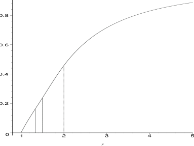
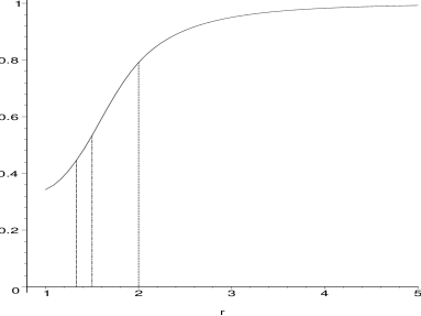
Figure 4: The edge probabilities $p_{\text{and}}(r)$ (left) and $p_{\text{or}}(r)$ (right) for $r\in[1,5]$.

To illustrate the limiting distribution, for example, $r=2$ yields

$$\frac{\sqrt{n}(\rho^{\text{and}}_{n}(2)-\mu_{\text{and}}(2))}{\sqrt{4\,\nu_{\text{and}}(2)}}=\sqrt{\frac{362880\,n}{58901}}\left(\rho^{\text{and}}_{n}(2)-\frac{11}{24}\right)\stackrel{{\scriptstyle\mathcal{L}}}{{\longrightarrow}}\mathcal{N}(0,1)$$

and

$$\frac{\sqrt{n}(\rho^{\text{or}}_{n}(2)-\mu_{\text{or}}(2))}{\sqrt{4\,\nu_{\text{or}}(2)}}=\sqrt{\frac{120960\,n}{13189}}\left(\rho^{\text{or}}_{n}(2)-\frac{19}{24}\right)\stackrel{{\scriptstyle\mathcal{L}}}{{\longrightarrow}}\mathcal{N}(0,1);$$

or equivalently,

$$\rho^{\text{and}}_{n}(2)\stackrel{{\scriptstyle\text{approx}}}{{\sim}}\mathcal{N}\left(\frac{11}{24},\frac{58901}{362880\,n}\right)\text{ and }\rho^{\text{or}}_{n}(2)\stackrel{{\scriptstyle\text{approx}}}{{\sim}}\mathcal{N}\left(\frac{19}{24},\frac{13189}{120960\,n}\right).$$

By construction of the underlying and reflexivity graphs, there is a natural ordering of the means of relative arc and edge densities.

Lemma 4.3.

The means of the relative edge densities and arc density (i.e., the edge and arc probabilities) have the following ordering: $p_{\text{and}}(r)<p(r)<p_{\text{or}}(r)$ for all $r\in[1,\infty)$. Furthermore, for $r=\infty$, we have $p_{\text{and}}(r)=p(r)=p_{\text{or}}(r)=1$.

Proof: Recall that $p_{\text{and}}(r)=\mathbf{E}[\rho_{n}^{\text{and}}(r)]=P(X_{2}\in N_{PE}^{r}(X_{1})\cap\Gamma_{1}^{r}(X_{1}))$, $p(r)=\mathbf{E}[\rho_{n}(r)]=P(X_{2}\in N_{PE}^{r}(X_{1}))$, and $p_{\text{or}}(r)=\mathbf{E}[\rho_{n}^{\text{or}}(r)]=P(X_{2}\in N_{PE}^{r}(X_{1})\cup\Gamma_{1}^{r}(X_{1}))$. And $\left[N_{PE}^{r}(X_{1})\cap\Gamma_{1}^{r}(X_{1})\right]\subseteq N_{PE}^{r}(X_{1})\subseteq\left[N_{PE}^{r}(X_{1})\cup\Gamma_{1}^{r}(X_{1})\right]$ with probability 1 for all $r\geq 1$ with equality holding for $r=\infty$ only. Then the desired result follows (See also Figure 3). $\blacksquare$

Note that the above lemma holds for all $X_{i}$ that has a continuous distribution on $T(\mathcal{Y}_{3})$. There is also a stochastic ordering for the relative edge and arc densities as follows.

Theorem 4.4.

For sufficiently small $r$, $\rho_{n}^{\text{and}}(r)<^{ST}\rho_{n}(r)<^{ST}\rho_{n}^{\text{or}}(r)$ as $n\rightarrow\infty$.

Proof: Above we have proved that $p_{\text{and}}(r)<p(r)<p_{\text{or}}(r)$ for all $r\in[1,\infty)$. For small $r$ ($r\lesssim 1.8$) the asymptotic variances have the same ordering, $4\,\nu_{\text{and}}(r)<4\,\nu(r)<4\,\nu_{\text{or}}(r)$. Since $\rho_{n}^{\text{and}}(r),\,\rho_{n}(r),\,\rho_{n}^{\text{or}}(r)$ are asymptotically normal, then the desired result follows (See also Figure 3). $\blacksquare$

We assess the accuracy of the asymptotic normality for finite sample data based on Monte Carlo simulations. We generate $n$ $\mathcal{X}$ points independently uniformly in the standard equilateral triangle $T_{e}$. For each data set generated, we calculate the relative edge density values for the reflexivity and underlying graphs based on the proportional-edge PCD with $r=2$. We replicate the above process $N_{mc}=1000$ times for each of $n=10,20$, and 100. We plot the histograms of the relative edge densities of the reflexivity and underlying graphs using the simulated data and the corresponding (asymptotic) normal curves in Figures 5 and 6, respectively. Notice that, for $r=2$, the normal approximation is accurate even for small $n$ although kurtosis may be indicated for $n=10$ in the reflexivity graph case, and skewness may be indicated for $n=10$ in the underlying graph case. We also investigate the behavior of the relative edge densities for extreme values of $n$ and $r$. So we generate $n=10$ $\mathcal{X}$ points and calculate the relative edge densities for $r=1.05$ and $r=5$. We repeat the above procedure $N_{mc}=10000$ times and plot the histograms of the relative edge densities in Figures 7 and 8, which demonstrate that severe skewness is obtained for these extreme values of $n$ and $r$. The finite sample variance and skewness may be derived analytically in much the same way as was $4\,\nu_{\text{and}}(r)$ (and $4\,\nu_{\text{or}}(r)]$) for the asymptotic variance. In fact, the exact distribution of $\rho^{\text{and}}_{n}(r)$ (and $\rho^{\text{or}}_{n}(r)$) is, in principle, available by successively conditioning on the values of the $X_{i}$. Alas, while the joint distribution of $h^{\text{and}}_{12}(r),h^{\text{and}}_{13}(r)$ (and $h^{\text{or}}_{12}(r),h^{\text{or}}_{13}(r)$) is available (see Figures 9 and 10), the joint distribution of $\{h^{\text{and}}_{ij}(r)\}_{1\leq i<j\leq n}$ (and $\{h^{\text{or}}_{ij}(r)\}_{1\leq i<j\leq n}$), and hence the calculation for the exact distribution of $\rho^{\text{and}}_{n}(r)$ (and $\rho^{\text{or}}_{n}(r)$), is extraordinarily tedious and lengthy for even small values of $n$.

\psfrag{Density}{\Huge{density}}\includegraphics{csr_andn10.ps}

\psfrag{Density}{\Huge{density}}\includegraphics{csr_andn20.ps}

\psfrag{Density}{\Huge{density}}\includegraphics{csr_andn100.ps}

Figure 5: Depicted are $\rho^{\text{and}}_{n}(2)\stackrel{{\scriptstyle\text{approx}}}{{\sim}}\mathcal{N}\left(\frac{11}{24},\frac{58901}{362880\,n}\right)$ for $n=10,\,20,\,100$ (left to right). Histograms are based on 1000 Monte Carlo replicates. Solid lines are the corresponding normal densities. Notice that the axes are differently scaled.

\psfrag{Density}{\Huge{density}}\includegraphics{csr_orn10.ps}

\psfrag{Density}{\Huge{density}}\includegraphics{csr_orn20.ps}

\psfrag{Density}{\Huge{density}}\includegraphics{csr_orn100.ps}

Figure 6: Depicted are $\rho^{\text{or}}_{n}(2)\stackrel{{\scriptstyle\text{approx}}}{{\sim}}\mathcal{N}\left(\frac{19}{24},\frac{13189}{120960\,n}\right)$ for $n=10,20,100$ (left to right). Histograms are based on 1000 Monte Carlo replicates. Solid lines are the corresponding normal densities. Notice that the axes are differently scaled.

\psfrag{Density}{\Huge{density}}\includegraphics{andskewn10r1.ps}

\psfrag{Density}{\Huge{density}}\includegraphics{andskewn10r5.ps}

Figure 7: Depicted are the histograms for 10000 Monte Carlo replicates of $\rho^{\text{and}}_{10}(1.05)$ (left) and $\rho^{\text{and}}_{10}(5)$ (right) indicating severe small sample skewness for extreme values of $r$. Notice that the vertical axes are differently scaled.

\psfrag{Density}{\Huge{density}}\includegraphics{orskewn10r1.ps}

\psfrag{Density}{\Huge{density}}\includegraphics{orskewn10r5.ps}

Figure 8: Depicted are the histograms for 10000 Monte Carlo replicates of $\rho^{\text{or}}_{10}(1)$ (left) and $\rho^{\text{or}}_{10}(5)$ (right) indicating severe small sample skewness for extreme values of $r$. Notice that the vertical axes are differently scaled.

\psfrag{r}{\Huge{$r$}}\includegraphics{P00and.eps}

\psfrag{r}{\Huge{$r$}}\includegraphics{P01and.eps}

\psfrag{r}{\Huge{$r$}}\includegraphics{P11and.eps}

Figure 9: The plots for the joint distribution of $h^{\text{and}}_{12}(r),h^{\text{and}}_{13}(r)$ for $r\in[1,5]$. Plotted are $P(h^{\text{and}}_{12}(r),h^{\text{and}}_{13}(r)=(0,0))$ (left), $P(h^{\text{and}}_{12}(r),h^{\text{and}}_{13}(r)=(1,0))=P(h^{\text{and}}_{12}(r),h^{\text{and}}_{13}(r)=(0,1))$ (middle), and $P(h^{\text{and}}_{12}(r),h^{\text{and}}_{13}(r)=(1,1))$ (right).

\psfrag{r}{\Huge{$r$}}\includegraphics{P00or.eps}

\psfrag{r}{\Huge{$r$}}\includegraphics{P01or.eps}

\psfrag{r}{\Huge{$r$}}\includegraphics{P11or.eps}

Figure 10: The plots for the joint distribution of $h^{\text{or}}_{12}(r),h^{\text{or}}_{13}(r)$ for $r\in[1,5]$. Plotted are $P(h^{\text{or}}_{12}(r),h^{\text{or}}_{13}(r)=(0,0))$ (left), $P(h^{\text{or}}_{12}(r),h^{\text{or}}_{13}(r)=(1,0))=P(h^{\text{or}}_{12}(r),h^{\text{or}}_{13}(r)=(0,1))$ (middle), and $P(h^{\text{or}}_{12}(r),h^{\text{or}}_{13}(r)=(1,1))$ (right).

Let $\gamma_{n}(r)$ be the domination number of the proportional-edge PCD based on $\mathcal{X}_{n}$ which is a random sample from $\mathcal{U}(T(\mathcal{Y}_{3}))$. Additionally, let $\gamma^{\text{and}}_{n}(r)$ and $\gamma^{\text{or}}_{n}(r)$ be the domination numbers of the reflexivity and underlying graphs based on the proportional-edge PCD, respectively. Then we have the following stochastic ordering for the domination numbers.

Theorem 4.5.

For all $r\in[1,\infty)$ and $n>1$, $\gamma^{\text{or}}_{n}(r)<^{ST}\gamma_{n}(r)<^{ST}\gamma^{\text{and}}_{n}(r)$.

Proof: For all $x\in T(\mathcal{Y}_{3})$, we have $\left[N_{PE}^{r}(x)\cap\Gamma^{r}_{1}(x)\right]\subseteq N_{PE}^{r}(x)\subseteq\left[N_{PE}^{r}(x)\cup\Gamma^{r}_{1}(x)\right]$. For $X\sim\mathcal{U}(T(\mathcal{Y}_{3}))$, we have $\left[N_{PE}^{r}(X)\cap\Gamma^{r}_{1}\left(X\right)\right]\subsetneq N_{PE}^{r}(X)\subsetneq\left[N_{PE}^{r}(X)\cup\Gamma^{r}_{1}\left(X\right)\right]$ a.s. Moreover, $\gamma_{n}(r)=1$ iff $\mathcal{X}_{n}\subset N_{PE}^{r}(X_{i})$ for some $i$; $\gamma^{\text{and}}_{n}(r)=1$ iff $\mathcal{X}_{n}\subset N_{PE}^{r}(X_{i})\cap\Gamma^{r}_{1}\left(X_{i}\right)$ for some $i$; and $\gamma^{\text{or}}_{n}(r)=1$ iff $\mathcal{X}_{n}\subset N_{PE}^{r}(X_{i})\cup\Gamma^{r}_{1}\left(X_{i}\right)$ for some $i$. So it follows that $P(\gamma^{\text{and}}_{n}(r)=1)<P(\gamma_{n}(r)=1)<P(\gamma^{\text{or}}_{n}(r)=1)$. Similarly, for all $x,y\in T(\mathcal{Y}_{3})$, we have $\Bigl{(}[N_{PE}^{r}(x)\cap\Gamma^{r}_{1}(x)]\cup[N_{PE}^{r}(y)\cap\Gamma^{r}_{1}(y)]\Bigr{)}\subseteq\left(N_{PE}^{r}(x)\cup N_{PE}^{r}(y)\right)\subseteq\Bigl{(}[N_{PE}^{r}(x)\cup\Gamma^{r}_{1}(x)]\cup[N_{PE}^{r}(y)\cup\Gamma^{r}_{1}(y)]\Bigr{)}$. For $X,Y\stackrel{{\scriptstyle iid}}{{\sim}}\mathcal{U}(T(\mathcal{Y}_{3}))$, we have $\Bigl{(}[N_{PE}^{r}(X)\cap\Gamma^{r}_{1}(X)]\cup[N_{PE}^{r}(Y)\cap\Gamma^{r}_{1}(Y)]\Bigr{)}\subsetneq\left(N_{PE}^{r}(X)\cup N_{PE}^{r}(Y)\right)\subsetneq\Bigl{(}[N_{PE}^{r}(X)\cup\Gamma^{r}_{1}(X)]\cup[N_{PE}^{r}(Y)\cup\Gamma^{r}_{1}(Y)]\Bigr{)}$ a.s. Moreover, $\gamma_{n}(r)\leq 2$ iff $\mathcal{X}_{n}\subset N_{PE}^{r}(X_{i})\cup N_{PE}^{r}(X_{j})$ for some $i\not=j$; $\gamma^{\text{and}}_{n}(r)\leq 2$ iff $\mathcal{X}_{n}\subset\Bigl{(}[N_{PE}^{r}(X_{i})\cap\Gamma^{r}_{1}\left(X_{i}\right)]\cup[N_{PE}^{r}(X_{j})\cap\Gamma^{r}_{1}\left(X_{j}\right)]\Bigr{)}$ for some $i\not=j$; and $\gamma^{\text{or}}_{n}(r)\leq 2$ iff $\mathcal{X}_{n}\subset\Bigl{(}[N_{PE}^{r}(X_{i})\cup\Gamma^{r}_{1}\left(X_{i}\right)]\cup[N_{PE}^{r}(X_{j})\cup\Gamma^{r}_{1}\left(X_{j}\right)]\Bigr{)}$ for some $i\not=j$. So it follows that $P(\gamma^{\text{and}}_{n}(r)\leq 2)<P(\gamma_{n}(r)\leq 2)<P(\gamma^{\text{or}}_{n}(r)\leq 2)$. Since $P(\gamma_{n}(r)\leq 3)=1$ (Ceyhan and Priebe, (2005)), it follows that $P(\gamma^{\text{or}}_{n}(r)\leq 3)=1$ also holds since $P(\gamma_{n}(r)\leq 3)\leq P(\gamma^{\text{or}}_{n}(r)\leq 3)$. Hence the desired stochastic ordering follows. $\blacksquare$

Note the stochastic ordering in the above theorem holds for any continuous distribution $F$ with support being in $T(\mathcal{Y}_{3})$. For $r=\infty$, we have $\gamma^{\text{or}}_{n}(r)=\gamma_{n}(r)=\gamma^{\text{and}}_{n}(r)=1$ a.s.

5 Multiple Triangle Case

Suppose $\mathcal{Y}_{m}$ is a finite set of $m>3$ points in $\mathbb{R}^{2}$. Consider the Delaunay triangulation (assumed to exist) of $\mathcal{Y}_{m}$. Let $T_{i}$ denote the $i^{th}$ Delaunay triangle, $J_{m}$ denote the number of triangles, and $C_{H}(\mathcal{Y}_{m})$ denote the convex hull of $\mathcal{Y}_{m}$. For $X_{i}\stackrel{{\scriptstyle iid}}{{\sim}}\mathcal{U}(C_{H}(\mathcal{Y}_{m}))$, $i=1,2,\ldots,n$, we construct the proportional-edge PCD, $D_{n,m}(r)$, using $N_{PE}^{r}(\cdot)$ as described in Section 3.5, where for $X_{i}\in T_{j}$, the three points in $\mathcal{Y}_{m}$ defining the Delaunay triangle $T_{j}$ are used as $\mathcal{Y}_{[j]}$. We investigate the relative edge densities of the underlying and reflexivity graphs based on the proportional-edge PCD. We consider various versions of the relative edge density in the multiple triangle case.

5.1 First Version of Relative Edge Density in the Multiple Triangle Case

For $J_{m}>1$, as in Section 3.6, let $\rho^{\text{and}}_{I,n}(r)=2\,\left|\mathcal{E}_{\text{and}}\right|/(n\,(n-1))$ and $\rho^{\text{or}}_{n}(r)=2\,\left|\mathcal{E}_{\text{or}}\right|/(n\,(n-1))$. Let $\mathcal{E}^{\text{and}}_{[i]}$ be the number of edges and $\rho^{\text{and}}_{{}_{[i]}}(r)$ be the relative edge density for triangle $i$ in the reflexivity graph case, and $\mathcal{E}^{\text{or}}_{[i]}$ and $\rho^{\text{or}}_{{}_{[i]}}(r)$ be similarly defined for underlying graph case. Let $n_{i}$ be the number of $X$ points in $T_{i}$ for $i=1,2,\ldots,J_{m}$. Letting $w_{i}=A(T_{i})/A(C_{H}(\mathcal{Y}_{m}))$ with $A(\cdot)$ being the area functional, we obtain the following as a corollary to Theorem 4.2.

Corollary 5.1.

For $r\in(1,\infty)$, the asymptotic distribution for $\rho^{\text{and}}_{I,n}(r)$ conditional on $\mathcal{Y}_{m}$ is given by

$$\sqrt{n}\left(\rho^{\text{and}}_{I,n}(r)-\widetilde{p}_{\text{and}}(m,r)\right)\stackrel{{\scriptstyle\mathcal{L}}}{{\longrightarrow}}\\ \mathcal{N}\left(0,4\,\widetilde{\nu}_{\text{and}}(m,r)\right),$$ (16)

as $n\rightarrow\infty$, where $\widetilde{p}_{\text{and}}(m,r)=p_{\text{and}}(r)\left(\sum_{i=1}^{J_{m}}w_{i}^{2}\right)$ and

$$\widetilde{\nu}_{\text{and}}(m,r)=\left[\nu_{\text{and}}(r)\left(\sum_{i=1}^{J_{m}}w_{i}^{3}\right)+\left(p_{\text{and}}(r)\right)^{2}\left(\sum_{i=1}^{J_{m}}w_{i}^{3}-\left(\sum_{j=1}^{J_{m}}w_{i}^{2}\right)^{2}\right)\right]$$

with $p_{\text{and}}(r)$ and $\nu_{\text{and}}(r)$ being as in Equations (12) and (14), respectively. The asymptotic distribution of $\rho^{\text{or}}_{I,n}(r)$ with $r\in[1,\infty)$ is similar.

The proof is provided in Appendix 4. By an appropriate application of the Jensen’s inequality, we see that $\sum_{i=1}^{J_{m}}w_{i}^{3}\geq\left(\sum_{i=1}^{J_{m}}w_{i}^{2}\right)^{2}.$ So the covariance above is zero iff $\nu_{\text{and}}(r)=0$ and $\sum_{i=1}^{J_{m}}w_{i}^{3}=\left(\sum_{i=1}^{J_{m}}w_{i}^{2}\right)^{2}$, so asymptotic normality may hold even though $\nu_{\text{and}}(r)=0$. That is, $\rho^{\text{and}}_{I,n}(r)$ has the asymptotic normality for $r\in\{1,\infty\}$ also provided that $\sum_{i=1}^{J_{m}}w_{i}^{3}>\left(\sum_{i=1}^{J_{m}}w_{i}^{2}\right)^{2}$. The same holds for the underlying graph case (for $r=\infty$).

5.2 Other Versions of Relative Edge Density in the Multiple Triangle Case

Let $\displaystyle\Xi^{\text{and}}_{n}(r):=\sum_{i=1}^{J_{m}}\frac{n_{i}\,(n_{i}-1)}{n\,(n-1)}\rho^{\text{and}}_{{}_{[i]}}(r)$. Then $\Xi^{\text{and}}_{n}(r)=\rho^{\text{and}}_{I,n}(r)$, since $\displaystyle\Xi^{\text{and}}_{n}(r)=\sum_{i=1}^{J_{m}}\frac{n_{i}\,(n_{i}-1)}{n\,(n-1)}\rho^{\text{and}}_{{}_{[i]}}(r)=\frac{\sum_{i=1}^{J_{m}}2\,|\mathcal{E}^{\text{and}}_{[i]}|}{n\,(n-1)}=\frac{2\,\left|\mathcal{E}_{\text{and}}\right|}{n\,(n-1)}=\rho^{\text{and}}_{I,n}(r)$. Similarly, we have $\Xi^{\text{or}}_{n}(r)=\rho^{\text{or}}_{n}(r)$.

Furthermore, let $\widehat{\Xi}^{\text{and}}_{n}:=\sum_{i=1}^{J_{m}}w_{i}^{2}\,\rho^{\text{and}}_{{}_{[i]}}(r)$ where $w_{i}$ is as in Section 5.1. So $\widehat{\Xi}^{\text{and}}_{n}$ a mixture of the $\rho^{\text{and}}_{{}_{[i]}}(r)$ values. Since the $\rho^{\text{and}}_{{}_{[i]}}(r)$ are asymptotically independent, $\Xi^{\text{and}}_{n}(r),\,\rho^{\text{and}}_{I,n}(r)$ are asymptotically normal; i.e., for large $n$ their distribution is approximately $\mathcal{N}\left(\widetilde{p}_{\text{and}}(m,r),4\,\widetilde{\nu}_{\text{and}}(m,r)/n\right)$. A similar result holds for the underlying graph case.

In Section 5.1, the denominator of $\rho^{\text{and}}_{I,n}(r)$ has $n(n-1)/2$ as the maximum number of edges possible. However, by definition, given the $n_{i}$ values, we can have a graph with at most $J_{m}$ complete components, each with order $n_{i}$ for $i=1,2,\ldots,J_{m}$. Then the maximum number of edges possible is $n_{t}:=\sum_{i=1}^{J_{m}}n_{i}\,(n_{i}-1)/2$ which suggests another version of edge density, namely, $\displaystyle\rho^{\text{and}}_{II,n}(r):=\frac{\left|E_{\text{and}}\right|}{n_{t}}$. Then $\displaystyle\rho^{\text{and}}_{II,n}(r)=\frac{\sum_{i=1}^{J_{m}}|E^{\text{and}}_{[i]}|}{n_{t}}=\sum_{i=1}^{J_{m}}\frac{n_{i}\,(n_{i}-1)}{2\,n_{t}}\,\rho^{\text{and}}_{{}_{[i]}}(r)$. Since $\frac{n_{i}\,(n_{i}-1)}{2\,n_{t}}\geq 0$ for each $i$, and $\displaystyle\sum_{i=1}^{J_{m}}\frac{n_{i}\,(n_{i}-1)}{2\,n_{t}}=1$, $\rho^{\text{and}}_{II,n}(r)$ is a mixture of the $\rho^{\text{and}}_{{}_{[i]}}(r)$. Then $\mathbf{E}\left[\rho^{\text{and}}_{II,n}(r)\right]=p_{\text{and}}(r)$. A similar result holds for the underlying graph case also.

Theorem 5.2.

The asymptotic distribution for $\rho^{\text{and}}_{II,n}(r)$ conditional on $\mathcal{Y}_{m}$ for $r\in(1,\infty)$ is given by

$$\sqrt{n}\left(\rho^{\text{and}}_{II,n}(r)-p_{\text{and}}(m,r)\right)\stackrel{{\scriptstyle\mathcal{L}}}{{\longrightarrow}}\\ \mathcal{N}\left(0,4\,\breve{\nu}_{\text{and}}(m,r)\right),$$ (17)

as $n\rightarrow\infty$, where $\breve{\nu}_{\text{and}}(m,r)=\left[\nu_{\text{and}}(r)\left(\sum_{i=1}^{J_{m}}w_{i}^{3}\right)\Big{/}\left(\sum_{i=1}^{J_{m}}w_{i}^{2}\right)^{2}\right]$ with $p_{\text{and}}(r)$ and $\nu_{\text{and}}(r)$ being as in Equations (12) and (14), respectively. The asymptotic distribution of $\rho^{\text{or}}_{II,n}(r)$ with $r\in[1,\infty)$ is similar.

The proof is provided in Appendix 5. Notice that the covariance $\breve{\nu}_{\text{and}}(m,r)$ is zero iff $\nu_{\text{and}}(r)=0$. The underlying graph case is similar.

Remark 5.3.

Comparison of Versions of Relative Edge Density in the Multiple Triangle Case: Among the versions of the relative edge density we considered, $\Xi^{\text{and}}_{n}(r)=\rho^{\text{and}}_{I,n}(r)$ for all $n>1$, and $\widehat{\Xi}^{\text{and}}_{n}$ and $\rho^{\text{and}}_{I,n}(r)$ are asymptotically equivalent (i.e., they have the same asymptotic distribution). However, $\rho^{\text{and}}_{I,n}(r)$ and $\rho^{\text{and}}_{II,n}(r)$ do not have the same distribution for finite or infinite $n$. But we have $\rho^{\text{and}}_{I,n}(r)=\frac{2\,n_{t}}{n(n-1)}\rho^{\text{and}}_{II,n}(r)$ and since $\sum_{i=1}^{J_{m}}w_{i}^{2}<1$, it follows that $\widetilde{p}_{\text{and}}(m,r)<\breve{p}_{\text{and}}(m,r)=p_{\text{and}}(r)$. Furthermore, since $\frac{2\,n_{t}}{n(n-1)}=\sum_{i=1}^{J_{m}}\frac{n_{i}(n_{i}-1)}{n(n-1)}\longrightarrow\sum_{i=1}^{J_{m}}w_{i}^{2}$ as $n_{i}\rightarrow\infty$, we have $\lim_{n_{i}\rightarrow\infty}\mathbf{Var}[\sqrt{n}\rho^{\text{and}}_{I,n}(r)]=\left(\sum_{i=1}^{J_{m}}w_{i}^{2}\right)^{2}\lim_{n_{i}\rightarrow\infty}\mathbf{Var}[\sqrt{n}\rho^{\text{and}}_{I,n}(r)]$. Hence $\breve{\nu}_{\text{and}}(m,r)\geq\widetilde{\nu}_{\text{and}}(m,r)$. Therefore, we recommend $\rho^{\text{and}}_{I,n}(r)$ for use in spatial pattern analysis in the multiple triangle case. Moreover, asymptotic normality might hold for $\rho^{\text{and}}_{I,n}(r)$ even if $\nu_{\text{and}}(r)=0$. $\square$

5.3 Extension to Higher Dimensions

The extension to $\mathbb{R}^{d}$ for $d>2$ is straightforward. Let $\mathcal{Y}_{d+1}=\{\mathsf{y}_{1},\mathsf{y}_{2},\ldots,\mathsf{y}_{d+1}\}$ be $d+1$ non-coplanar points. Denote the simplex formed by these $d+1$ points as $\mathfrak{S}(\mathcal{Y}_{d+1})$. A simplex is the simplest polytope in $\mathbb{R}^{d}$ having $d+1$ vertices, $d\,(d+1)/2$ edges and $d+1$ faces of dimension $(d-1)$. For $r\in[1,\infty]$, define the proportional-edge proximity map as follows. Given a point $x$ in $\mathfrak{S}(\mathcal{Y}_{d+1})$, let $\mathsf{y}:=\arg\min_{\mathsf{y}\in\mathcal{Y}_{d+1}}\mbox{volume}(Q_{\mathsf{y}}(x))$ where $Q_{\mathsf{y}}(x)$ is the polytope with vertices being the $d\,(d+1)/2$ midpoints of the edges, the vertex $\mathsf{y}$ and $x$. That is, the vertex region for vertex $v$ is the polytope with vertices given by $v$ and the midpoints of the edges. Let $v(x)$ be the vertex in whose region $x$ falls. If $x$ falls on the boundary of two vertex regions or at the center of mass, we assign $v(x)$ arbitrarily. Let $\varphi(x)$ be the face opposite to vertex $v(x)$, and $\eta(v(x),x)$ be the hyperplane parallel to $\varphi(x)$ which contains $x$. Let $d(v(x),\eta(v(x),x))$ be the Euclidean distance from $v(x)$ to $\eta(v(x),x)$. For $r\in[1,\infty)$, let $\eta_{r}(v(x),x)$ be the hyperplane parallel to $\varphi(x)$ such that

$$d(v(x),\eta_{r}(v(x),x))=r\,d(v(x),\eta(v(x),x))\text{ and }d(\eta(v(x),x),\eta_{r}(v(x),x))<d(v(x),\eta_{r}(v(x),x)).$$

Let $\mathfrak{S}_{r}(x)$ be the polytope similar to and with the same orientation as $\mathfrak{S}$ having $v(x)$ as a vertex and $\eta_{r}(v(x),x)$ as the opposite face. Then the proportional-edge proximity region $N_{PE}^{r}(x):=\mathfrak{S}_{r}(x)\cap\mathfrak{S}(\mathcal{Y}_{d+1})$. Furthermore, let $\zeta_{i}(x)$ be the hyperplane such that $\zeta_{i}(x)\cap\mathfrak{S}(\mathcal{Y}_{d+1})\not=\emptyset$ and $r\,d(\mathsf{y}_{i},\zeta_{i}(x))=d(\mathsf{y}_{i},\eta(\mathsf{y}_{i},x))$ for $i=1,2,\ldots,d+1$. Then $\Gamma_{1}^{r}(x)\cap R(\mathsf{y}_{i})=\{z\in R(\mathsf{y}_{i}):d(\mathsf{y}_{i},\eta(\mathsf{y}_{i},z))\geq d(\mathsf{y}_{i},\zeta_{i}(x)\}$, for $i=1,2,3$. Hence $\Gamma_{1}^{r}(x)=\bigcup_{j=1}^{d+1}(\Gamma_{1}^{r}(x)\cap R(\mathsf{y}_{i}))$. Notice that $r\geq 1$ implies $x\in N_{PE}^{r}(x)$ and $x\in\Gamma_{1}^{r}(x)$.

Theorem 4.1 generalizes, so that any simplex $\mathfrak{S}$ in $\mathbb{R}^{d}$ can be transformed into a regular polytope (with edges being equal in length and faces being equal in volume) preserving uniformity. Delaunay triangulation becomes Delaunay tessellation in $\mathbb{R}^{d}$, provided no more than $d+1$ points being cospherical (lying on the boundary of the same sphere). In particular, with $d=3$, the general simplex is a tetrahedron (4 vertices, 4 triangular faces and 6 edges), which can be mapped into a regular tetrahedron (4 faces are equilateral triangles) with vertices $(0,0,0)\,(1,0,0)\,(1/2,\sqrt{3}/2,0),\,(1/2,\sqrt{3}/4,\sqrt{3}/2)$.

Asymptotic normality of the $U$-statistic holds for $d>2$ in both underlying cases.

6 Discussion and Conclusions

In this article, we demonstrate that the relative edge density of random graphs and relative arc density of random digraphs are one-sample $U$-statistics of degree 2. Then, we specify the conditions under which the asymptotic normality of the relative densities holds for the random graphs and digraphs. We consider the asymptotic distribution of the relative edge density of the underlying and reflexivity graphs based on (parameterized) proportional-edge proximity catch digraphs (PE-PCDs). In particular, we consider the reflexivity and underlying graphs based on the proportional-edge PCD; and derive the asymptotic distribution of the relative edge density using the central limit theory of $U$-statistics. We compute the asymptotic mean and variance of the limiting normal distribution for uniform data based on detailed geometric calculations. Moreover, we compare the asymptotic distributions of the relative edge densities of the underlying and reflexivity graphs and of the relative arc density of the PCDs.

The PCDs have applications in classification and spatial pattern analysis. Ceyhan et al., (2006) used that the relative (arc) density of the PE-PCDs for testing bivariate spatial patterns. The relative edge densities of the underlying and reflexivity graphs based on this PCD can be employed for the same purpose. More specifically, the relative edge densities can be employed for testing the complete spatial randomness (CSR) of two or more classes of points against the segregation or association of the points from the classes. CSR is roughly defined as the lack of spatial interaction between the points in a given study area. In particular, the null hypothesis can be assumed to be CSR of $\mathcal{X}$ points, i.e., the uniformness of $\mathcal{X}$ points in the convex hull of $\mathcal{Y}$ points. Segregation is the pattern in which points of one class tend to cluster together, i.e., form one-class clumps. On the other hand, association is the pattern in which the points of one class tend to occur more frequently around points from the other class. Under the segregation alternative, the $\mathcal{X}$ points will tend to be further away from $\mathcal{Y}$ points and under the association alternative $\mathcal{X}$ points will tend to cluster around the $\mathcal{Y}$ points. Such patterns can be detected by the test statistics based on the relative edge densities, since under segregation we expect them to be smaller, and under association they tend to be larger. The underlying and reflexivity graphs can also be used in pattern classification as outlined in Priebe et al., 2003a . Moreover, the methodology described here is also applicable to PCDs in higher dimensions.

APPENDIX

Appendix 1: The Asymptotic Variance of Relative Edge Density for the Reflexivity Graph

The variance of $h^{\text{and}}_{12}(r)$, denoted as $\mathbf{Var}_{\text{and}}(r)=\mathbf{Var}\left[h^{\text{and}}_{12}(r)\right]$, is as follows:

$$\mathbf{Var}_{\text{and}}(r)=\varphi^{\text{and}}_{1,1}(r)\mathbf{I}(r\in[1,4/3))+\varphi^{\text{and}}_{1,2}(r)\mathbf{I}(r\in[4/3,3/2))+\varphi^{\text{and}}_{1,3}(r)\mathbf{I}(r\in[3/2,2))+\varphi^{\text{and}}_{1,4}(r)\mathbf{I}(r\in[2,\infty))$$

where $\varphi^{\text{and}}_{1,1}(r)=-{\frac{(5\,r^{6}-153\,r^{5}+393\,r^{4}-423\,r^{3}-54\,r^{2}+360\,r-128)(447\,r^{4}-261\,r^{3}+54\,r^{2}+5\,r^{6}-153\,r^{5}+360\,r-128)}{2916\,r^{4}(r+2)^{2}(r+1)^{2}}}$,
$\varphi^{\text{and}}_{1,2}(r)=-{\frac{(101\,r^{5}-801\,r^{4}+1302\,r^{3}-732\,r^{2}-536\,r+672)(1518\,r^{3}-84\,r^{2}-104\,r+101\,r^{5}-801\,r^{4}+672)}{46656\,r^{2}(r+2)^{2}(r+1)^{2}}}$,
$\varphi^{\text{and}}_{1,3}(r)=-{\frac{(r^{8}-13\,r^{7}+30\,r^{6}+148\,r^{5}-448\,r^{4}+264\,r^{3}+288\,r^{2}-368\,r+96)(22\,r^{6}+124\,r^{5}-464\,r^{4}+r^{8}-13\,r^{7}+264\,r^{3}+288\,r^{2}-368\,r+96)}{64\,r^{8}(r+2)^{2}(r+1)^{2}}}$,
$\varphi^{\text{and}}_{1,4}(r)={\frac{(r^{5}+r^{4}-3\,r^{3}-3\,r^{2}+6\,r-2)(3\,r^{3}+3\,r^{2}-6\,r+2)}{r^{8}(r+1)^{2}}}$. Note that $\mathbf{Var}_{\text{and}}(r=1)=0$ and $\lim_{r\rightarrow\infty}\mathbf{Var}_{\text{and}}(r)=0$ (at rate $O(r^{-2})$), and $\operatorname{argsup}_{r\in[1,\infty)}\mathbf{Var}_{\text{and}}(r)\approx 2.1126$ with $\sup\mathbf{Var}_{\text{and}}(r)=0.25$.

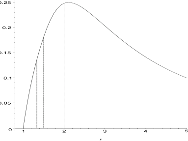
Figure 11: $\mathbf{Var}\left[h^{\text{and}}_{12}(r)\right]$ (left) and $\mathbf{Var}\left[h^{\text{or}}_{12}(r)\right]$ (right) as a function of $r$ for $r\in[1,5]$.

The asymptotic variance for the reflexivity graph case is

$$\nu_{\text{and}}(r):=\mathbf{Cov}\left[h^{\text{and}}_{12}(r),h^{\text{and}}_{13}(r)\right]=\sum_{i=1}^{11}\vartheta^{\text{and}}_{i}(r)\,\mathbf{I}(\mathcal{I}_{i})$$

where

$$\vartheta^{\text{and}}_{1}(r)=-\frac{1}{58320\,(2\,r^{2}+1)(r+2)^{2}(r+1)^{3}r^{6}}\,((r-1)^{2}(972\,r^{19}+8748\,r^{18}+44456\,r^{17}+140328\,r^{16}+121371\,r^{15}\\ -412117\,r^{14}-27145\,r^{13}-4503501\,r^{12}+1336147\,r^{11}+10640999\,r^{10}-982009\,r^{9}-6677105\,r^{8}-2274458\,r^{7}\\ -1150162\,r^{6}+249126\,r^{5}+1232530\,r^{4}+1234372\,r^{3}+226776\,r^{2}-184944\,r-81920))$$

$$\vartheta^{\text{and}}_{2}(r)=-\frac{1}{116640\,(2\,r^{2}+1)(r+2)^{2}(r+1)^{3}r^{6}}\,(486\,r^{21}+3402\,r^{20}-269\,r^{19}-45155\,r^{18}-118850\,r^{17}+443518\,r^{16}\\ +3251855\,r^{15}-13836295\,r^{14}+13434672\,r^{13}+11140788\,r^{12}-27667544\,r^{11}+13293088\,r^{10}+7159710\,r^{9}-\\ 13013598\,r^{8}+4185440\,r^{7}+3262952\,r^{6}+586636\,r^{5}-1616444\,r^{4}-680120\,r^{3}-55952\,r^{2}+219936\,r+49152)$$

$$\vartheta^{\text{and}}_{3}(r)=-\frac{1}{116640\,(2\,r^{2}+1)(r+2)^{2}(r+1)^{3}r^{6}}\,(486\,r^{21}+3402\,r^{20}-269\,r^{19}-45155\,r^{18}-118850\,r^{17}+443518\,r^{16}\\ +2751855\,r^{15}-13736295\,r^{14}+18084672\,r^{13}+8770788\,r^{12}-43009544\,r^{11}+24604048\,r^{10}+27137438\,r^{9}-30889822\,r^{8}\\ -2832544\,r^{7}+11101160\,r^{6}-4168820\,r^{5}+2364868\,r^{4}+2305864\,r^{3}-3041936\,r^{2}+219936\,r+49152)$$

$$\vartheta^{\text{and}}_{4}(r)=-\frac{1}{58320\,(r+2)^{3}(r^{2}-2)(2\,r^{2}+1)(r+1)^{3}r^{6}}\,(3632\,r^{22}+25632\,r^{21}-60328\,r^{20}-441888\,r^{19}+1353430\,r^{18}\\ -297666\,r^{17}-4791125\,r^{16}+12849927\,r^{15}-10894618\,r^{14}-26295324\,r^{13}+62283823\,r^{12}-2280753\,r^{11}-81700012\,r^{10}\\ +32551926\,r^{9}+39974410\,r^{8}-11284026\,r^{7}-5806580\,r^{6}-9167580\,r^{5}-2004944\,r^{4}+4646688\,r^{3}+1931776\,r^{2}-489024\,r-98304)$$

$$\vartheta^{\text{and}}_{5}(r)=\vartheta^{\text{and}}_{6}(r)=-\frac{1}{58320\,(r+2)^{3}(2\,r^{2}+1)(r^{2}+1)(r+1)^{3}r^{6}}\,(3632\,r^{22}+25632\,r^{21}-49432\,r^{20}-364992\,r^{19}+958940\,r^{18}\\ -1167012\,r^{17}+1200518\,r^{16}+5424126\,r^{15}-23566328\,r^{14}+23837088\,r^{13}+11797395\,r^{12}-41623065\,r^{11}+39261953\,r^{10}\\ -8239197\,r^{9}-30178496\,r^{8}+27901506\,r^{7}-4936170\,r^{6}+61038\,r^{5}+4719720\,r^{4}-5513952\,r^{3}+340736\,r^{2}+23328\,r+65536)$$

$$\vartheta^{\text{and}}_{7}(r)=\frac{1}{466560\,(r+2)^{3}(2\,r^{2}+1)(r^{2}+1)(r+1)^{3}r^{5}}\,(1562\,r^{21}-11142\,r^{20}-103099\,r^{19}+2105697\,r^{18}-9774118\,r^{17}+\\ 10220280\,r^{16}+27825711\,r^{15}-69243129\,r^{14}+81624200\,r^{13}-76052574\,r^{12}-65530400\,r^{11}+262451196\,r^{10}-178092280\,r^{9}\\ -69106464\,r^{8}+158439568\,r^{7}-97568688\,r^{6}+12246288\,r^{5}+17591952\,r^{4}-21111616\,r^{3}+15628032\,r^{2}-2545664\,r+993024)$$

$$\vartheta^{\text{and}}_{8}(r)=-\frac{1}{1920\,(r+2)^{3}(r^{2}+1)(2\,r^{2}+1)(r+1)^{3}r^{10}}\,(2\,r^{26}-30\,r^{25}-2395\,r^{23}+281\,r^{24}+8770\,r^{22}+29528\,r^{21}-268053\,r^{20}+\\ 245667\,r^{19}+2066216\,r^{18}-5313494\,r^{17}-1589216\,r^{16}+18512684\,r^{15}-18946136\,r^{14}-2665248\,r^{13}+22789584\,r^{12}-\\ 32987760\,r^{11}+20482512\,r^{10}+13109584\,r^{9}-28084416\,r^{8}+17326976\,r^{7}-3864576\,r^{6}-4579328\,r^{5}+6666240\,r^{4}-3576320\,r^{3}\\ +635904\,r^{2}-116736\,r+61440)$$

$$\vartheta^{\text{and}}_{9}(r)=-\frac{1}{1920\,(r+2)^{3}(r^{2}+1)(2\,r^{2}+1)(r+1)^{3}r^{10}}\,(2\,r^{26}-30\,r^{25}-2395\,r^{23}281\,r^{24}+8258\,r^{22}+31064\,r^{21}-262677\,r^{20}+\\ 225443\,r^{19}+2052136\,r^{18}-5219030\,r^{17}-1608928\,r^{16}+18337836\,r^{15}-18837080\,r^{14}-2598688\,r^{13}+22736336\,r^{12}-\\ 32858736\,r^{11}+20384720\,r^{10}+12930896\,r^{9}-27988416\,r^{8}+17416832\,r^{7}-3862784\,r^{6}-4575488\,r^{5}+6638848\,r^{4}-3603200\,r^{3}\\ +640512\,r^{2}-107520\,r+63488)$$

$$\vartheta^{\text{and}}_{10}(r)=-\frac{1}{1920\,(r+2)^{3}(r-1)(r+1)^{3}(2\,r^{2}-1)r^{10}}\,(2\,r^{25}+307\,r^{23}-32\,r^{24}-2612\,r^{22}+11572\,r^{21}+21934\,r^{20}-328867\,r^{19}+\\ 524994\,r^{18}+2446870\,r^{17}-8676180\,r^{16}-437020\,r^{15}+36944680\,r^{14}-40677696\,r^{13}-44860384\,r^{12}+106256352\,r^{11}-\\ 15515040\,r^{10}-98636848\,r^{9}+66358080\,r^{8}+27142272\,r^{7}-42614272\,r^{6}+7781120\,r^{5}+7327232\,r^{4}-3388672\,r^{3}+\\ 430592\,r^{2}-171008\,r+63488)$$

$$\vartheta^{\text{and}}_{11}(r)=\frac{1}{15\,(2\,r^{2}-1)(r+1)^{3}r^{10}}\,(30\,r^{13}+90\,r^{12}-127\,r^{11}-621\,r^{10}+320\,r^{9}+1568\,r^{8}-858\,r^{7}-1370\,r^{6}+909\,r^{5}+\\ 295\,r^{4}-292\,r^{3}+44\,r^{2}+6\,r-2)$$

and $\mathcal{I}_{1}=[1,2/\sqrt{3}),\;\mathcal{I}_{2}=[2/\sqrt{3},6/5),\;\mathcal{I}_{3}=[6/5,\sqrt{5}-1),\;\mathcal{I}_{4}=[\sqrt{5}-1,(6+2\,\sqrt{2})/7),\;\mathcal{I}_{5}=[(6+2\,\sqrt{2})/7,4/3),\;\mathcal{I}_{6}=[4/3,(6+\sqrt{15})/7),\;\mathcal{I}_{7}=[(6+\sqrt{15})/7,3/2),\;\mathcal{I}_{8}=[3/2,(1+\sqrt{5})/2),\;\mathcal{I}_{9}=[(1+\sqrt{5})/2,1+1/\sqrt{2}),\;\mathcal{I}_{10}=[1+1/\sqrt{2},2),\;\mathcal{I}_{11}=[2,\infty)$. See Figure 3. Note that $\mathbf{Cov}_{\text{and}}(r=1)=0$ and $\lim_{r\rightarrow\infty}\nu_{\text{and}}(r)=0$ (at rate $O(r^{-2})$), and $\operatorname{argsup}_{r\in[1,\infty)}\nu_{\text{and}}(r)\approx 2.69$ with $\sup\nu_{\text{and}}(r)\approx.0537$.

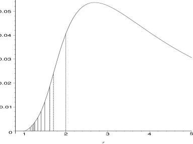
Figure 12: $\nu_{\text{and}}(r)=\mathbf{Cov}\left[h^{\text{and}}_{12}(r),h^{\text{and}}_{13}(r)\right]$ (left) and $\nu_{\text{or}}(r)=\mathbf{Cov}\left[h^{\text{or}}_{12}(r),h^{\text{or}}_{13}(r)\right]$ (right) as a function of $r$ for $r\in[1,5]$.

Appendix 2: The Asymptotic Variance of Relative Edge Density for the Underlying Graph

The variance of $h^{\text{or}}_{12}(r)$, denoted as $\mathbf{Var}_{\text{or}}(r)=\mathbf{Var}\left[h^{\text{or}}_{12}(r)\right]$, is as follows:

$$\mathbf{Var}_{\text{or}}(r)=\varphi^{\text{or}}_{1,1}(r)\mathbf{I}(r\in[1,4/3))+\varphi^{\text{or}}_{1,2}(r)\mathbf{I}(r\in[4/3,3/2))+\varphi^{\text{or}}_{1,3}(r)\mathbf{I}(r\in[3/2,2))+\varphi^{\text{or}}_{1,4}(r)\mathbf{I}(r\in[2,\infty))$$

where $\varphi^{\text{or}}_{1,1}(r)=-\frac{(47\,r^{6}-195\,r^{5}+860\,r^{4}-846\,r^{3}-108\,r^{2}+720\,r-256)(752\,r^{4}-1170\,r^{3}-324\,r^{2}+47\,r^{6}-195\,r^{5}+720\,r-256)}{11664\,r^{4}(r+2)^{2}(r+1)^{2}}$,
$\varphi^{\text{or}}_{1,2}(r)=-\frac{(175\,r^{5}-579\,r^{4}+1450\,r^{3}-732\,r^{2}-536\,r+672)(1234\,r^{3}-1380\,r^{2}-968\,r+175\,r^{5}-579\,r^{4}+672)}{46656\,r^{2}(r+2)^{2}(r+1)^{2}}$,
$\varphi^{\text{or}}_{1,3}(r)=-\frac{(3\,r^{8}-7\,r^{7}-30\,r^{6}+84\,r^{5}-264\,r^{4}+304\,r^{3}+144\,r^{2}-368\,r+96)(-22\,r^{6}+108\,r^{5}-248\,r^{4}+3\,r^{8}-7\,r^{7}+304\,r^{3}+144\,r^{2}-368\,r+96)}{64\,r^{8}(r+2)^{2}(r+1)^{2}}$,

$\varphi^{\text{or}}_{1,4}(r)=2\,\frac{(r^{5}+r^{4}-6\,r+2)(3\,r-1)}{r^{8}(r+1)^{2}}$. See Figure 11.

Note that $\mathbf{Var}_{\text{or}}(r=1)=2627/11664$ and $\lim_{r\rightarrow\infty}\mathbf{Var}_{\text{or}}(r)=0$ (at rate $O(r^{-4})$), and $\operatorname{argsup}_{r\in[1,\infty)}\mathbf{Var}_{\text{or}}(r)\approx 1.44$ with $\sup\mathbf{Var}_{\text{or}}(r)\approx.25$.

The asymptotic variance for the underlying graph is

$$\nu_{\text{or}}(r):=\mathbf{Cov}[h^{\text{or}}_{12}(r),h^{\text{or}}_{13}(r)]=\sum_{i=1}^{11}\vartheta^{\text{or}}_{i}(r)\,\mathbf{I}(\mathcal{I}_{i})$$

where

$$\vartheta^{\text{or}}_{1}(r)=-\frac{1}{58320\,(r^{2}+1)(2\,r^{2}+1)(r+1)^{3}(r+2)^{3}r^{6}}\,(1458\,r^{22}+13122\,r^{21}+50731\,r^{20}-84225\,r^{19}-19193\,r^{18}-1823223\,r^{17}+\\ 5576151\,r^{16}+2978697\,r^{15}-33432692\,r^{14}+37427862\,r^{13}+15883834\,r^{12}-60944766\,r^{11}+49876417\,r^{10}-1754523\,r^{9}-\\ 36606859\,r^{8}+32338215\,r^{7}-10290256\,r^{6}-2234754\,r^{5}+7085471\,r^{4}-5608569\,r^{3}+1645826\,r^{2}-132876\,r+30824)$$

$$\vartheta^{\text{or}}_{2}(r)=\vartheta^{\text{or}}_{3}(r)=-\frac{1}{116640\,(r^{2}+1)(2\,r^{2}+1)(r+1)^{3}(r+2)^{3}r^{6}}\,(1458\,r^{22}+13122\,r^{21}+62825\,r^{20}-175011\,r^{19}+156014\,r^{18}-\\ 3300900\,r^{17}+11053023\,r^{16}+5055135\,r^{15}-67685050\,r^{14}+75243552\,r^{13}+33155180\,r^{12}-120628524\,r^{11}+99831906\,r^{10}-\\ 4883958\,r^{9}-74801558\,r^{8}+64360782\,r^{7}-19812000\,r^{6}-3667716\,r^{5}+14541630\,r^{4}-11254002\,r^{3}+3070468\,r^{2}-413208\,r+28880)$$

$$\vartheta^{\text{or}}_{4}(r)=-\frac{1}{58320\,(r^{2}+1)(2\,r^{2}+1)(r^{2}-2)(r+2)^{3}(r+1)^{3}r^{6}}\,(972\,r^{24}+8748\,r^{23}+29590\,r^{22}-149106\,r^{21}-36820\,r^{20}-\\ 986280\,r^{19}+5942884\,r^{18}+2883672\,r^{17}-47189711\,r^{16}+43450125\,r^{15}+85975304\,r^{14}-156173934\,r^{13}+27378901\,r^{12}+123606417\,r^{11}\\ -152209261\,r^{10}+64653597\,r^{9}+56621894\,r^{8}-88962768\,r^{7}+43754559\,r^{6}-5940597\,r^{5}-13006396\,r^{4}+17019366\,r^{3}-7037340\,r^{2}+\\ 413208\,r-28880)$$

$$\vartheta^{\text{or}}_{5}(r)=-\frac{1}{58320\,(r^{2}+1)(2\,r^{2}+1)(r+1)^{3}(r+2)^{3}r^{6}}\,(972\,r^{22}+8748\,r^{21}+31534\,r^{20}-131610\,r^{19}+261546\,r^{18}-1552026\,r^{17}+\\ 3745643\,r^{16}+4573731\,r^{15}-29416804\,r^{14}+26163354\,r^{13}+19600850\,r^{12}-43126062\,r^{11}+31497249\,r^{10}-7381467\,r^{9}-\\ 22237963\,r^{8}+26778663\,r^{7}-9107024\,r^{6}-115074\,r^{5}+3136927\,r^{4}-5055609\,r^{3}+2292994\,r^{2}+14580\,r-1944)$$

$$\vartheta^{\text{or}}_{6}(r)=\frac{1}{233280\,(r^{2}+1)(2\,r^{2}+1)(r+1)^{3}(r+2)^{3}r^{6}}\,(486\,r^{22}-7290\,r^{21}-181459\,r^{20}+1024401\,r^{19}-2691213\,r^{18}+3921057\,r^{17}+\\ 1844321\,r^{16}-33347697\,r^{15}+80028903\,r^{14}-29292735\,r^{13}-98093906\,r^{12}+125034492\,r^{11}-46658244\,r^{10}-57216612\,r^{9}+\\ 88057996\,r^{8}-26383068\,r^{7}-12851392\,r^{6}+14179848\,r^{5}-8656508\,r^{4}+1593828\,r^{3}+134136\,r^{2}-58320\,r+7776)$$

$$\vartheta^{\text{or}}_{7}(r)=\frac{1}{233280\,(r+2)^{3}(r^{2}+1)(2\,r^{2}+1)(r+1)^{3}(r-1)r^{6}}\,(486\,r^{23}-7776\,r^{22}-174169\,r^{21}+1205860\,r^{20}-4656806\,r^{19}+\\ 8763566\,r^{18}+7460036\,r^{17}-63559490\,r^{16}+91134324\,r^{15}+18516450\,r^{14}-122708655\,r^{13}+18577230\,r^{12}+80410332\,r^{11}-19357704\,r^{10}-\\ 39129236\,r^{9}+75311048\,r^{8}-77449360\,r^{7}+4053376\,r^{6}+48283912\,r^{5}-40690240\,r^{4}+17736336\,r^{3}-4315680\,r^{2}+544320\,r-31104)$$

$$\vartheta^{\text{or}}_{8}(r)=\frac{1}{960\,(r+2)^{3}(r^{2}+1)(2\,r^{2}+1)(r+1)^{3}r^{8}}\,(2\,r^{24}-30\,r^{23}-161\,r^{22}+107\,r^{21}+4137\,r^{20}-10685\,r^{19}+8367\,r^{18}+\\ 78713\,r^{17}-450859\,r^{16}+697707\,r^{15}+517846\,r^{14}-3723120\,r^{13}+6565124\,r^{12}-1468692\,r^{11}-8695792\,r^{10}+9535720\,r^{9}-\\ 6773160\,r^{8}+526744\,r^{7}+10691376\,r^{6}-7797264\,r^{5}+1137696\,r^{4}+523712\,r^{3}-2687872\,r^{2}+1701888\,r-245760)$$

$$\vartheta^{\text{or}}_{9}(r)=\frac{1}{960\,(2\,r^{2}+1)(r+1)^{2}(r+2)^{3}(r^{2}+1)r^{10}}\,(2\,r^{25}-32\,r^{24}-129\,r^{23}+236\,r^{22}+4157\,r^{21}-15610\,r^{20}+21289\,r^{19}+\\ 67536\,r^{18}-511355\,r^{17}+1161830\,r^{16}-634128\,r^{15}-3001568\,r^{14}+9512164\,r^{13}-11014136\,r^{12}+2344968\,r^{11}+7126240\,r^{10}-\\ 13850504\,r^{9}+14466592\,r^{8}-3823216\,r^{7}-4018976\,r^{6}+5155776\,r^{5}-4633984\,r^{4}+1959808\,r^{3}-244480\,r^{2}-3584\,r-1024)$$

$$\vartheta^{\text{or}}_{10}(r)=\frac{1}{960\,(2\,r^{2}-1)(r+2)^{3}(r-1)(r+1)^{2}r^{10}}\,(2\,r^{24}-34\,r^{23}-101\,r^{22}+433\,r^{21}+5400\,r^{20}-26982\,r^{19}+23049\,r^{18}+\\ 166787\,r^{17}-717366\,r^{16}+1196092\,r^{15}+89468\,r^{14}-5130844\,r^{13}+12748688\,r^{12}-11274744\,r^{11}-12243496\,r^{10}+\\ 33980568\,r^{9}-14886656\,r^{8}-19910592\,r^{7}+20667776\,r^{6}-1262208\,r^{5}-5402752\,r^{4}+2217088\,r^{3}-235776\,r^{2}-2560\,r-1024)$$

$$\vartheta^{\text{or}}_{11}(r)=\frac{2}{15}\,{\frac{180\,r^{8}-48\,r^{7}-648\,r^{6}+396\,r^{5}+214\,r^{4}-190\,r^{3}+39\,r^{2}-4\,r+1}{(2\,r^{2}-1)(r+1)^{2}r^{10}}}$$

and $\mathcal{I}_{1}=[1,2/\sqrt{3}),\;\mathcal{I}_{2}=[2/\sqrt{3},6/5),\;\mathcal{I}_{3}=[6/5,\sqrt{5}-1),\;\mathcal{I}_{4}=[\sqrt{5}-1,(6+2\,\sqrt{2})/7),\;\mathcal{I}_{5}=[(6+2\,\sqrt{2})/7,4/3),\;\mathcal{I}_{6}=[4/3,(6+\sqrt{15})/7),\;\mathcal{I}_{7}=[(6+\sqrt{15})/7,3/2),\;\mathcal{I}_{8}=[3/2,(1+\sqrt{5})/2),\;\mathcal{I}_{9}=[(1+\sqrt{5})/2,1+1/\sqrt{2}),\;\mathcal{I}_{10}=[1+1/\sqrt{2},2),\;\mathcal{I}_{11}=[2,\infty)$. See Figure 3. Note that $\mathbf{Cov}_{\text{or}}(r=1)=1/3240$ and $\lim_{r\rightarrow\infty}\nu_{\text{or}}(r)=0$ (at rate $O(r^{-6})$), and $\operatorname{argsup}_{r\in[1,\infty)}\nu_{\text{or}}(r)\approx 1.765$ with $\sup\nu_{\text{or}}(r)\approx.0318$.

Appendix 3: Derivation of the Asymptotic Mean and Variance for Uniform Data

In the standard equilateral triangle, let $\mathsf{y}_{1}=(0,0)$, $\mathsf{y}_{2}=(1,0)$, $\mathsf{y}_{3}=\bigl{(}1/2,\sqrt{3}/2\bigr{)}$, $M_{C}$ be the center of mass, $M_{i}$ be the midpoints of the edges $e_{i}$ for $i=1,2,3$. Then $M_{C}=\bigl{(}1/2,\sqrt{3}/6\bigr{)}$, $M_{1}=\bigl{(}3/4,\sqrt{3}/4\bigr{)}$, $M_{2}=\bigl{(}1/4,\sqrt{3}/4\bigr{)}$, $M_{3}=(1/2,0)$. Let $\mathcal{X}_{n}$ be a random sample of size $n$ from $\mathcal{U}(T(\mathcal{Y}_{3}))$. For $x_{1}=(u,v)$, $\ell_{r}(x_{1})=r\,v+r\,\sqrt{3}\,u-\sqrt{3}\,x.$ Next, let $N_{1}:=\ell_{r}(x_{1})\cap e_{3}$ and $N_{2}:=\ell_{r}(x_{1})\cap e_{2}$.

Appendix 3.1: Derivation of $p_{\text{and}}(r)$ and $\nu_{\text{and}}(r)$ for Uniform Data

Derivation of $\mu_{\text{and}}(r)$ in Theorem 4.2

First we find $\mu_{\text{and}}(r)$ for $r\in(1,\infty)$. Observe that, by symmetry,

$$\mu_{\text{and}}(r)=P\bigl{(}X_{2}\in N_{PE}^{r}(X_{1})\cap\Gamma_{1}^{r}(X_{1})\bigr{)}=6\,P\bigl{(}X_{2}\in N_{\mathcal{Y}}^{r}(X_{1})\cap\Gamma_{1}^{r}(X_{1}),X_{1}\in T_{s}\bigr{)}$$

where $T_{s}$ is the triangle with vertices $\mathsf{y}_{1}$, $M_{3}$, and $M_{C}$. Let $\ell_{s}(r,x)$ be the line such that $r\,d(\mathsf{y}_{1},\ell_{s}(r,x))=d(\mathsf{y}_{1},e_{1})$, so $\ell_{s}(r,x)=\sqrt{3}\,(1/r-x)$. Then if $x_{1}\in T_{s}$ is above $\ell_{s}(r,x)$ then $N_{PE}^{r}(x_{1})=T(\mathcal{Y}_{3})$, otherwise, $N_{PE}^{r}(x_{1})\subsetneq T(\mathcal{Y}_{3})$.

Figure 13: The cases for relative position of $\ell_{s}(r,x)$ with various $r$ values. These are the prototypes for various types of $N_{PE}^{r}(x_{1})$.

Figure 14: The prototypes of the six cases of $\Gamma^{r}_{1}\left(x\right)$ for $x\in T_{s}$ for $r\in[1,4/3)$.

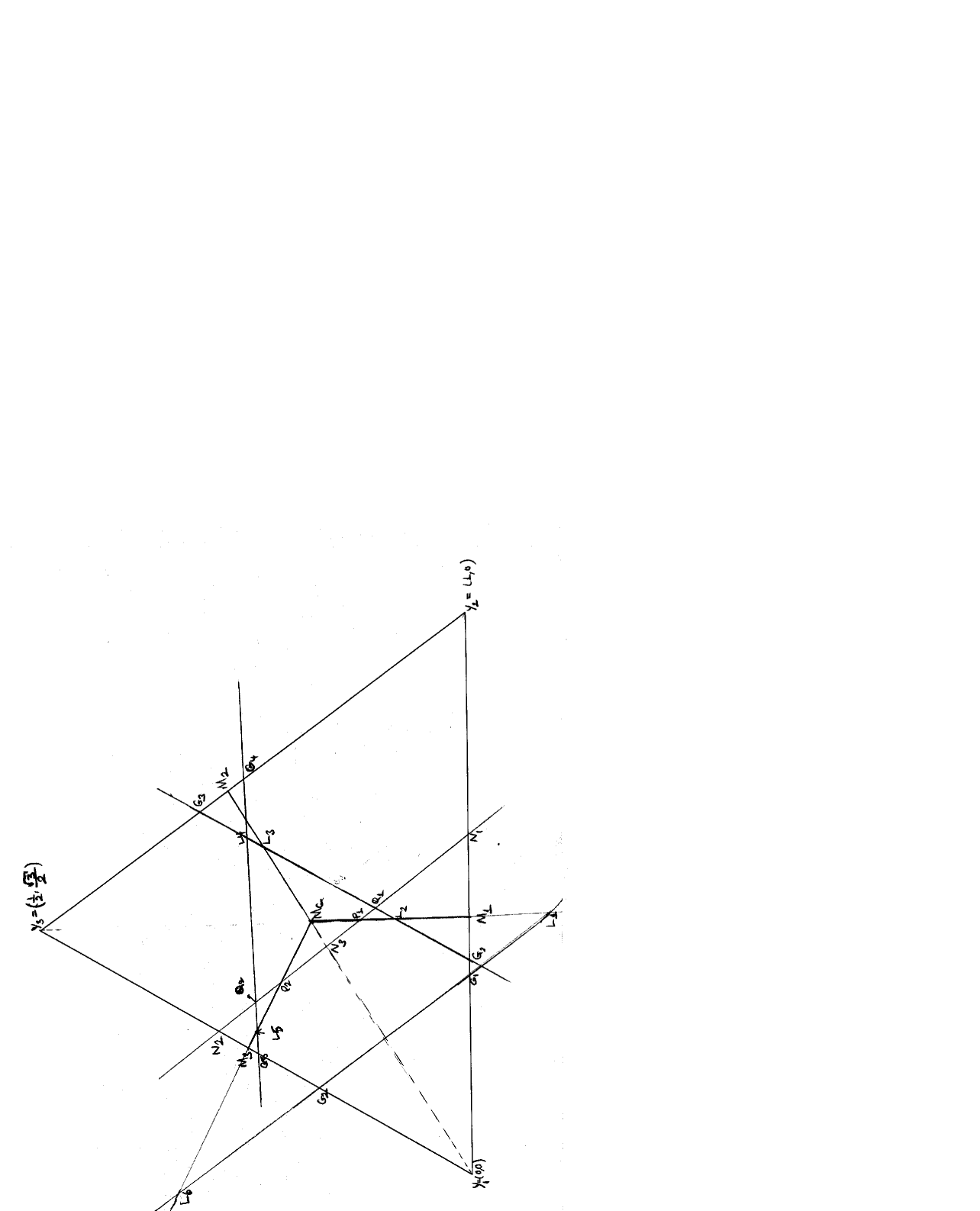
Figure 15: An illustration of the vertices for possible types of $N_{PE}^{r}(x_{1})\cap\Gamma_{1}^{r}(x_{1})$ for $x_{1}\in T_{s}$.

To compute $\mu_{\text{and}}(r)$, we need to consider various cases for $N_{PE}^{r}(X_{1})$ and $\Gamma_{1}^{r}(X_{1})$ given $X_{1}=(x,y)\in T_{s}$. See Figures 13 and 14. For any $x=(u,v)\in T(\mathcal{Y})$, $\Gamma^{r}_{1}(x)$ is a convex or nonconvex polygon. Let $\xi_{i}(r,x)$ be the line between $x$ and the vertex $\mathsf{y}_{i}$ parallel to the edge $e_{i}$ such that $r\,d(\mathsf{y}_{i},\xi_{i}(r,x))=d(\mathsf{y}_{i},\ell_{r}(x))\text{ for }i=1,2,3.$ Then $\Gamma^{r}_{1}(x)\cap R(\mathsf{y}_{i})$ is bounded by $\xi_{i}(r,x)$ and the median lines. For $x=(u,v)$, $\xi_{1}(r,x)=-\sqrt{3}\,x+(v+\sqrt{3}\,u)/r,\;\xi_{2}(r,x)=(v+\sqrt{3}r\,(x-1)+\sqrt{3}(1-u))/r\text{ and }\xi_{3}(r,x)=(\sqrt{3}(r-1)+2\,v)/(2\,r).$ For $r\in\Bigl{[}6/5,\sqrt{5}-1)$, there are six cases regarding $\Gamma_{1}^{r}(x)$ and one case for $N_{PE}^{r}(x)$. See Figure 14 for the prototypes of these six cases of $\Gamma_{1}\left(x,N_{\mathcal{Y}}^{r}\right)$. For the reflexivity graph case, we determine the possible types of $N_{PE}^{r}(x_{1})\cap\Gamma_{1}^{r}(x_{1})$ for $x_{1}\in T_{s}$. Depending on the location of $x_{1}$ and the value of the parameter $r$, $N_{PE}^{r}(x_{1})\cap\Gamma_{1}^{r}(x_{1})$ regions are polygons with various vertices. See Figure 15 for the illustration of these vertices and below for their explicit forms.

$G_{1}=\left({\frac{\sqrt{3}y+3\,x}{3r}},0\right)$, $G_{2}=\left(-{\frac{\sqrt{3}y-3\,r+3-3\,x}{3r}},0\right)$, $G_{3}=\left(-{\frac{\sqrt{3}y-6\,r+3-3\,x}{6r}},-{\frac{\sqrt{3}\left(-\sqrt{3}y-3+3\,x\right)}{6r}}\right)$, $G_{4}=\Bigl{(}{\frac{\left(\sqrt{3}r+\sqrt{3}-2\,y\right)\sqrt{3}}{6r}},\\ {\frac{\sqrt{3}\left(3\,r-3+2\,\sqrt{3}y\right)}{6r}}\Bigr{)}$, $G_{5}=\left({\frac{\left(\sqrt{3}r-\sqrt{3}+2\,y\right)\sqrt{3}}{6r}},{\frac{\sqrt{3}\left(3\,r-3+2\,\sqrt{3}y\right)}{6r}}\right)$, $G_{6}=\left({\frac{\sqrt{3}y+3\,x}{6r}},{\frac{\sqrt{3}\left(\sqrt{3}y+3\,x\right)}{6r}}\right)$;

$P_{1}=\left(1/2,\sqrt{3}/6\,\left(2\,\sqrt{3}r\,y+6\,r\,x-3\right)\right)$, and $P_{2}=\left(-1/2+(\sqrt{3}r\,y+3\,r\,x)/2,-\sqrt{3}/6\,\left(-3+\sqrt{3}r\,y+3\,r\,x\right)\right)$;

$L_{1}=\left(1/2,{\frac{\sqrt{3}\left(2\,\sqrt{3}y+6\,x-3\,r\right)}{6r}}\right)$, $L_{2}=\left(1/2,-{\frac{\left(-2\,\sqrt{3}y-6+6\,x+3\,r\right)\sqrt{3}}{6r}}\right)$, $L_{3}=\left(-{\frac{\sqrt{3}y-3\,r+3-3\,x}{2r}},{\frac{\sqrt{3}\left(3\,r-\sqrt{3}y-3+3\,x\right)}{6r}}\right)$, $L_{4}=\left({\frac{3\,r-3+2\,\sqrt{3}y}{2r}},{\frac{\sqrt{3}\left(3\,r-3+2\,\sqrt{3}y\right)}{6r}}\right)$, $L_{5}=\left(-{\frac{r-3+2\,\sqrt{3}y}{2r}},{\frac{\sqrt{3}\left(3\,r-3+2\,\sqrt{3}y\right)}{6r}}\right)$, and $L_{6}=\left({\frac{-r+\sqrt{3}y+3\,x}{2r}},-{\frac{\sqrt{3}\left(\sqrt{3}y+3\,x-3\,r\right)}{6r}}\right)$; $N_{1}=\left(\sqrt{3}r\,y/3+r\,x,0\right)$, $N_{2}=\left(\sqrt{3}r\,y/6+r\,x/2,\sqrt{3}\left(\sqrt{3}y/6+3\,x\right)r\right)$, and
$N_{3}=\left(\sqrt{3}r\,y/4+3\,r\,x/4,\sqrt{3}\left(\sqrt{3}y/12+3\,x\right)r\right)$; and $Q_{1}=\left({\frac{\sqrt{3}r^{2}y+3\,r^{2}x-\sqrt{3}y+3\,r-3+3\,x}{6r}},{\frac{\left(\sqrt{3}r^{2}y+3\,r^{2}x+\sqrt{3}y-3\,r+3-3\,x\right)\sqrt{3}}{6r}}\right)$,
and $Q_{2}=\left({\frac{2\,\sqrt{3}r^{2}y+6\,r^{2}x-3\,r+3-2\,\sqrt{3}y}{6r}},{\frac{\sqrt{3}\left(3\,r-3+2\,\sqrt{3}y\right)}{6r}}\right)$.

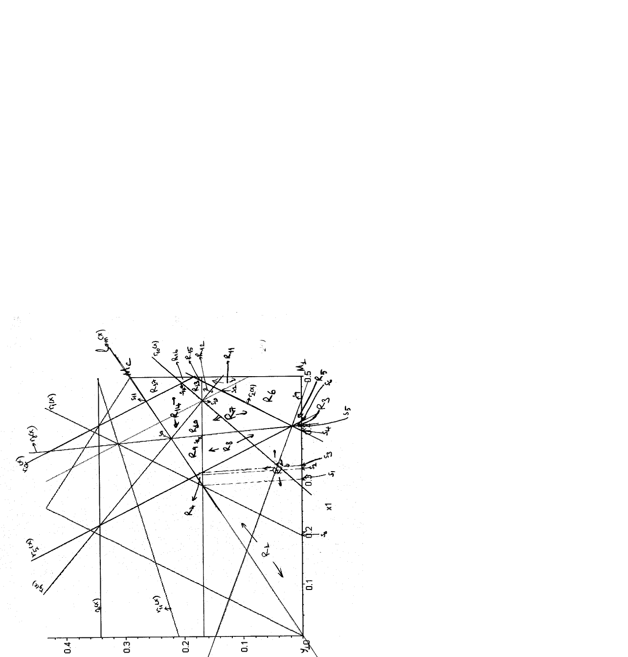
Figure 16: Prototype regions $R_{i}$ for various types of $N_{PE}^{r}(x_{1})\cap\Gamma_{1}^{r}(x_{1})$ and the corresponding points whose $x$-coordinates are $s_{k}$ values.

Let $\mathscr{P}(a_{1},a_{2},\ldots,a_{n})$ denote the polygon with vertices $a_{1},a_{2},\ldots,a_{n}$. For $r\in\bigl{[}1,4/3\bigr{)}$, there are 14 cases to consider for calculation of $p_{\text{and}}(r)$ in the reflexivity graph version. Each of these cases correspond to the regions in Figure 16, where Case 1 corresponds to $R_{i}$ for $i=1,2,3,4$, and Case $j$ for $j>1$ corresponds to $R_{j+3}$ for $j=1,2,\ldots,14$. These regions are bounded by various combinations of the lines defined below.

Let $\ell_{am}(x)$ be the line joining $\mathsf{y}_{1}$ to $M_{C}$, then $\ell_{am}(x)=\sqrt{3}x/3$. Let also $r_{1}(x)=\sqrt{3}\left(2\,r+3\,x-3\right)/3$, $r_{2}(x)=\sqrt{3}/2-\sqrt{3}r/3$, $r_{3}(x)=\left(2\,x-2+r\right)\sqrt{3}/2$, $r_{4}(x)=\sqrt{3}/2-\sqrt{3}r/4$, $r_{5}(x)=-{\frac{\sqrt{3}\left(2\,r\,x-1\right)}{2r}}$, $r_{6}(x)=-{\frac{\sqrt{3}\left(-2+3\,r\,x\right)}{3r}}$, $r_{7}(x)=-{\frac{\left(1+r^{2}x-r-x\right)\sqrt{3}}{r^{2}+1}}$, $r_{8}(x)=-{\frac{\left(r^{2}x-1+x\right)\sqrt{3}}{r^{2}-1}}$, $r_{9}(x)=-{\frac{\left(r^{2}x-1\right)\sqrt{3}}{r^{2}+2}}$, $r_{10}(x)=-{\frac{\left(-2\,r+2+r^{2}x\right)\sqrt{3}}{-4+r^{2}}}$, $r_{11}(x)=-{\frac{\left(-2\,r+2-2\,x+r^{2}x\right)\sqrt{3}}{r^{2}+2}}$, $r_{12}(x)=-\left(2\,x-r\right)\sqrt{3}/2$, and $r_{13}(x)=-\left(-1+x\right)\sqrt{3}/3$. Furthermore, to determine the integration limits, we specify the $x$-coordinate of the boundaries of these regions using $s_{k}$ for $k=0,1,\ldots,14$. See also Figure 16 for an illustration of these points whose explicit forms are provided below.

$s_{0}=1-2\,r/3$, $s_{1}=3/2-r$, $s_{2}=3/(8\,r)$, $s_{3}={\frac{-3\,r+2\,r^{2}+3}{6r}}$, $s_{4}=1-r/2$, $s_{5}={\frac{2\,r-r^{2}+1}{4r}}$, $s_{6}=1/(2\,r)$, $s_{7}=\frac{3}{2\,\left(2\,r^{2}+1\right)}$, $s_{8}={\frac{9-3\,r^{2}+2\,r^{3}-2\,r}{6(r^{2}+1)}}$, $s_{9}=1/\left(r+1\right)$, $s_{10}={\frac{-3\,r+2\,r^{2}+4}{6r}}$, $s_{11}=3\,r/8$, $s_{12}={\frac{6\,r-3\,r^{2}+4}{12r}}$, $s_{13}=3/2-5\,r/6$, and $s_{14}=r-1/2-r^{3}/8$.

Below, we compute $P(X_{2}\in N_{PE}^{r}(X_{1})\cap\Gamma_{1}^{r}(X_{1}),X_{1}\in T_{s})$ for each of the 14 cases: Case 1:

$$P(X_{2}\in N_{PE}^{r}(X_{1})\cap\Gamma_{1}^{r}(X_{1}),X_{1}\in T_{s})=\left(\int_{0}^{s_{2}}\int_{0}^{\ell_{am}(x)}+\int_{s_{2}}^{s_{6}}\int_{0}^{r_{5}(x)}\right)\frac{A(\mathscr{P}(G_{1},N_{1},N_{2},G_{6}))}{A(T(\mathcal{Y}_{3}))^{2}}dydx=\\ {\frac{\left(r-1\right)\left(r+1\right)\left(r^{2}+1\right)}{64\,r^{6}}}$$

where $A(\mathscr{P}(G_{1},N_{1},N_{2},G_{6}))=\sqrt{3}/36\,\left(\sqrt{3}y+3\,x\right)^{2}r^{2}-{\frac{\sqrt{3}\left(\sqrt{3}y+3\,x\right)^{2}}{36\,r^{2}}}$.

Case 2:

$$P(X_{2}\in N_{PE}^{r}(X_{1})\cap\Gamma_{1}^{r}(X_{1}),X_{1}\in T_{s})=\left(\int_{s_{5}}^{s_{6}}\int_{r_{5}(x)}^{r_{7}(x)}+\int_{s_{6}}^{s_{9}}\int_{0}^{r_{7}(x)}\right)\frac{A(\mathscr{P}(G_{1},N_{1},P_{2},M_{3},G_{6}))}{A(T(\mathcal{Y}_{3}))^{2}}dydx=\\ {\frac{\left(9\,r^{5}+23\,r^{4}+24\,r^{3}+24\,r^{2}+13\,r+3\right)\left(r-1\right)^{4}}{96\,r^{6}\left(r+1\right)^{3}}}$$

where $A(\mathscr{P}(G_{1},N_{1},P_{2},M_{3},G_{6}))=-{\frac{\sqrt{3}\left(-4\,r^{3}\sqrt{3}y-12\,r^{3}x+2\,r^{4}\,y^{2}+4\,r^{4}\sqrt{3}y\,x+6\,r^{4}x^{2}+3\,r^{2}+2\,y^{2}+4\,\sqrt{3}y\,x+6\,x^{2}\right)}{24\,r^{2}}}$.

Case 3:

$$P(X_{2}\in N_{PE}^{r}(X_{1})\cap\Gamma_{1}^{r}(X_{1}),X_{1}\in T_{s})=\\ \left(\int_{s_{5}}^{s_{9}}\int_{r_{7}(x)}^{r_{3}(x)}+\int_{s_{9}}^{s_{12}}\int_{0}^{r_{3}(x)}+\int_{s_{12}}^{1/2}\int_{0}^{r_{6}(x)}\right)\frac{A(\mathscr{P}(G_{1},G_{2},Q_{1},P_{2},M_{3},G_{6}))}{A(T(\mathcal{Y}_{3}))^{2}}dydx=\\ {\frac{324\,r^{11}-1620\,r^{10}-618\,r^{9}+4626\,r^{8}+990\,r^{7}-2454\,r^{6}+2703\,r^{5}-5571\,r^{4}-3827\,r^{3}+1455\,r^{2}+3072\,r+1024}{7776\,\left(r+1\right)^{3}r^{6}}}$$

where $A(\mathscr{P}(G_{1},G_{2},Q_{1},P_{2},M_{3},G_{6}))=-\Bigl{[}\sqrt{3}\bigl{(}-4\,\sqrt{3}r\,y-12\,x+4\,y^{2}+4\,r^{2}\,y^{2}-12\,r+9\,r^{2}+12\,r\,x+4\,r^{4}\,y^{2}-12\,x^{2}r^{2}-24\,r^{3}x+12\,r^{4}x^{2}+8\,r^{4}\sqrt{3}y\,x+12\,x^{2}+12\,r^{2}x+6-8\,r^{3}\sqrt{3}y+4\,\sqrt{3}y+4\,\sqrt{3}r^{2}y\bigr{)}\Bigr{]}\Big{/}\Bigl{[}24\,r^{2}\Bigr{]}$.

Case 4:

$$P(X_{2}\in N_{PE}^{r}(X_{1})\cap\Gamma_{1}^{r}(X_{1}),X_{1}\in T_{s})=\\ \left(\int_{s_{8}}^{s_{5}}\int_{r_{8}(x)}^{r_{2}(x)}+\int_{s_{5}}^{s_{10}}\int_{r_{3}(x)}^{r_{2}(x)}+\int_{s_{10}}^{s_{12}}\int_{r_{3}(x)}^{r_{6}(x)}\right)\frac{A(\mathscr{P}(G_{1},M_{1},L_{2},Q_{1},P_{2},M_{3},G_{6}))}{A(T(\mathcal{Y}_{3}))^{2}}dydx=\\ \Bigl{[}512+138240\,r^{7}+3654\,r^{12}-255\,r^{8}+43008\,r^{3}-12369\,r^{2}-86387\,r^{4}-193581\,r^{6}+148224\,r^{5}-100608\,r^{9}+94802\,r^{10}-\\ 35328\,r^{11}\Bigr{]}\Big{/}\Bigl{[}7776\,\left(r^{2}+1\right)^{3}r^{6}\Bigr{]}$$

where $A(\mathscr{P}(G_{1},M_{1},L_{2},Q_{1},P_{2},M_{3},G_{6}))=-\Bigl{[}\sqrt{3}\bigl{(}6\,x+3\,r^{2}-2\,\sqrt{3}y+2\,\sqrt{3}r^{2}y+2\,r^{4}\,y^{2}-4\,r^{3}\sqrt{3}y+4\,\sqrt{3}y\,x+2\,r^{2}y^{2}+4\,r^{4}\sqrt{3}y\,x-6\,x^{2}r^{2}-12\,r^{3}x+6\,r^{4}x^{2}+6\,r^{2}x-3\bigr{)}\Bigr{]}\Big{/}\Bigl{[}12\,r^{2}\Bigr{]}$.

Case 5:

$$P(X_{2}\in N_{PE}^{r}(X_{1})\cap\Gamma_{1}^{r}(X_{1}),X_{1}\in T_{s})=\left(\int_{s_{3}}^{s_{8}}\int_{r_{5}(x)}^{r_{2}(x)}+\int_{s_{8}}^{s_{5}}\int_{r_{5}(x)}^{r_{8}(x)}\right)\frac{A(\mathscr{P}(G_{1},M_{1},P_{1},P_{2},M_{3},G_{6}))}{A(T(\mathcal{Y}_{3}))^{2}}dydx=\\ -{\frac{\left(177\,r^{8}-648\,r^{7}+570\,r^{6}-360\,r^{5}+28\,r^{4}-24\,r^{3}+174\,r^{2}+72\,r+27\right)\left(-12\,r+7\,r^{2}+3\right)^{2}}{7776\,\left(r^{2}+1\right)^{3}r^{6}}}$$

where $A(\mathscr{P}(G_{1},M_{1},L_{2},Q_{1},P_{2},M_{3},G_{6}))=-{\frac{\sqrt{3}\left(-4\,r^{3}\sqrt{3}y-12\,r^{3}x+3\,r^{2}+6\,r^{4}\sqrt{3}y\,x+9\,r^{4}x^{2}+3\,r^{4}\,y^{2}+\,y^{2}+2\,\sqrt{3}y\,x+3\,x^{2}\right)}{12\,r^{2}}}$.

Case 6:

$$P(X_{2}\in N_{PE}^{r}(X_{1})\cap\Gamma_{1}^{r}(X_{1}),X_{1}\in T_{s})=\\ \left(\int_{s_{2}}^{s_{3}}\int_{r_{5}(x)}^{\ell_{am}(x)}+\int_{s_{3}}^{s_{7}}\int_{r_{2}(x)}^{\ell_{am}(x)}+\int_{s_{7}}^{s_{8}}\int_{r_{2}(x)}^{r_{8}(x)}\right)\frac{A(\mathscr{P}(G_{1},M_{1},P_{1},P_{2},M_{3},G_{6}))}{A(T(\mathcal{Y}_{3}))^{2}}dydx=\\ \Bigl{[}137472\,r^{18}-952704\,r^{17}+2792712\,r^{16}-5116608\,r^{15}+7057828\,r^{14}-7725792\,r^{13}+7022682\,r^{12}-5484816\,r^{11}+\\ 3631995\,r^{10}-2213712\,r^{9}+1213271\,r^{8}-578976\,r^{7}+292518\,r^{6}-101952\,r^{5}+36612\,r^{4}-11664\,r^{3}+3051\,r^{2}-1296\,r+243\Bigr{]}\Big{/}\\ \Bigl{[}\left(15552\,r^{2}+1\right)^{3}\left(2\,r^{2}+1\right)^{3}r^{6}\Bigr{]}$$

where $A(\mathscr{P}(G_{1},M_{1},P_{1},P_{2},M_{3},G_{6}))=-{\frac{\sqrt{3}\left(-4\,r^{3}\sqrt{3}y-12\,r^{3}x+3\,r^{2}+6\,r^{4}\sqrt{3}y\,x+9\,r^{4}x^{2}+3\,r^{4}\,y^{2}+\,y^{2}+2\,\sqrt{3}y\,x+3\,x^{2}\right)}{12\,r^{2}}}$.

Case 7:

$$P(X_{2}\in N_{PE}^{r}(X_{1})\cap\Gamma_{1}^{r}(X_{1}),X_{1}\in T_{s})=\left(\int_{s_{7}}^{s_{8}}\int_{r_{8}(x)}^{r_{9}(x)}+\int_{s_{8}}^{s_{10}}\int_{r_{2}(x)}^{r_{9}(x)}\right)\frac{A(\mathscr{P}(G_{1},M_{1},L_{2},Q_{1},P_{2},M_{3},G_{6}))}{A(T(\mathcal{Y}_{3}))^{2}}dydx=\\ -{\frac{4\left(100\,r^{11}-408\,r^{10}+454\,r^{9}-564\,r^{8}+283\,r^{7}-108\,r^{6}-34\,r^{5}+204\,r^{4}-r^{3}+132\,r^{2}+26\,r+24\right)\left(2\,r-1\right)^{2}\left(r-1\right)^{2}}{243\left(r^{2}+1\right)^{3}r^{3}\left(2\,r^{2}+1\right)^{3}}}$$

where $A(\mathscr{P}(G_{1},M_{1},L_{2},Q_{1},P_{2},M_{3},G_{6}))=-\Bigl{[}\sqrt{3}\bigl{(}6\,x+3\,r^{2}-2\,\sqrt{3}y+2\,\sqrt{3}r^{2}y+2\,r^{4}\,y^{2}-4\,r^{3}\sqrt{3}y+4\,\sqrt{3}y\,x+2\,r^{2}y^{2}+4\,r^{4}\sqrt{3}y\,x-6\,x^{2}r^{2}-12\,r^{3}x+6\,r^{4}x^{2}+6\,r^{2}x-3\bigr{)}\Bigr{]}\Big{/}\Bigl{[}12\,r^{2}\Bigr{]}$.

Case 8:

$$P(X_{2}\in N_{PE}^{r}(X_{1})\cap\Gamma_{1}^{r}(X_{1}),X_{1}\in T_{s})=\left(\int_{s_{12}}^{s_{13}}\int_{r_{6}(x)}^{r_{3}(x)}+\int_{s_{13}}^{1/2}\int_{r_{6}(x)}^{r_{2}(x)}\right)\frac{A(\mathscr{P}(G_{1},G_{2},Q_{1},N_{3},M_{C},M_{3},G_{6}))}{A(T(\mathcal{Y}_{3}))^{2}}dydx=\\ \Bigl{[}\left(-2+r\right)\bigl{(}2369\,r^{11}-11342\,r^{10}+29934\,r^{9}-50340\,r^{8}+54056\,r^{7}-51824\,r^{6}+48320\,r^{5}-20864\,r^{4}-640\,r^{3}\\ -1280\,r^{2}+512\,r+1024\bigr{)}\Bigr{]}\Big{/}\Bigl{[}15552\,r^{6}\Bigr{]}$$

where $A(\mathscr{P}(G_{1},G_{2},Q_{1},N_{3},M_{C},M_{3},G_{6}))=-\Bigl{[}\sqrt{3}\bigl{(}4\,\sqrt{3}r^{2}y-12\,x-12\,r+5\,r^{2}+12\,r\,x+4\,y^{2}-12\,x^{2}r^{2}+4\,r^{2}\,y^{2}+r^{4}\,y^{2}+2\,r^{4}\sqrt{3}y\,x-4\,r^{3}\sqrt{3}y+6-12\,r^{3}x+3\,r^{4}x^{2}+12\,x^{2}+12\,r^{2}x-4\,\sqrt{3}r\,y+4\,\sqrt{3}y\bigr{)}\Bigr{]}\Big{/}\Bigl{[}24\,r^{2}\Bigr{]}$.

Case 9:

$$P(X_{2}\in N_{PE}^{r}(X_{1})\cap\Gamma_{1}^{r}(X_{1}),X_{1}\in T_{s})=\left(\int_{s_{10}}^{s_{12}}\int_{r_{6}(x)}^{r_{2}(x)}+\int_{s_{12}}^{s_{13}}\int_{r_{3}(x)}^{r_{2}(x)}\right)\frac{A(\mathscr{P}(G_{1},M_{1},L_{2},Q_{1},N_{3},M_{C},M_{3},G_{6}))}{A(T(\mathcal{Y}_{3}))^{2}}dydx=\\ -{\frac{\left(49\,r^{8}-168\,r^{7}+354\,r^{6}-528\,r^{5}+236\,r^{4}-96\,r^{3}-224\,r^{2}+384\,r+64\right)\left(-12\,r+7\,r^{2}+4\right)^{2}}{15552\,r^{6}}}$$

where $A(\mathscr{P}(G_{1},M_{1},L_{2},Q_{1},N_{3},M_{C},M_{3},G_{6}))=-\Bigl{[}\sqrt{3}\bigl{(}8\,\sqrt{3}y\,x+4\,\sqrt{3}r^{2}y+12\,x+2\,r^{2}-12\,x^{2}r^{2}-4\,r^{3}\sqrt{3}y-12\,r^{3}x+3\,r^{4}x^{2}+r^{4}\,y^{2}+2\,r^{4}\sqrt{3}y\,x+12\,r^{2}x-6-4\,\sqrt{3}y+4\,r^{2}\,y^{2}\bigr{)}\Bigr{]}\Big{/}\Bigl{[}24\,r^{2}\Bigr{]}$.

Case 10:

$$P(X_{2}\in N_{PE}^{r}(X_{1})\cap\Gamma_{1}^{r}(X_{1}),X_{1}\in T_{s})=\\ \left(\int_{s_{10}}^{s_{14}}\int_{r_{2}(x)}^{r_{10}(x)}+\int_{s_{14}}^{s_{13}}\int_{r_{2}(x)}^{r_{12}(x)}+\int_{s_{13}}^{1/2}\int_{r_{3}(x)}^{r_{12}(x)}\right)\frac{A(\mathscr{P}(G_{1},M_{1},L_{2},Q_{1},N_{3},L_{4},L_{5},M_{3},G_{6}))}{A(T(\mathcal{Y}_{3}))^{2}}dydx=\\ -{\frac{6144+195456\,r^{6}+324\,r^{11}-76720\,r^{7}-801792\,r^{2}+217856\,r+946432\,r^{3}-239904\,r^{5}-275328\,r^{4}+39408\,r^{8}-11849\,r^{9}}{31104\,r^{3}}}$$

where $A(\mathscr{P}(G_{1},M_{1},L_{2},Q_{1},N_{3},L_{4},L_{5},M_{3},G_{6}))=-\Bigl{[}\sqrt{3}\bigl{(}4\,\sqrt{3}r^{2}y+8\,\sqrt{3}y\,x+4\,r^{2}\,y^{2}-16\,\sqrt{3}r\,y-4\,r^{3}\sqrt{3}y-24\,y^{2}+12\,x+24\,r-6\,r^{2}-12\,x^{2}r^{2}-12\,r^{3}x+3\,r^{4}x^{2}+12\,r^{2}x+20\,\sqrt{3}y+2\,r^{4}\sqrt{3}y\,x+r^{4}\,y^{2}-24\bigr{)}\Bigr{]}\Big{/}\Bigl{[}24\,r^{2}\Bigr{]}$.

Case 11:

$$P(X_{2}\in N_{PE}^{r}(X_{1})\cap\Gamma_{1}^{r}(X_{1}),X_{1}\in T_{s})=\\ \left(\int_{s_{7}}^{s_{11}}\int_{r_{9}(x)}^{\ell_{am}(x)}+\int_{s_{11}}^{s_{10}}\int_{r_{9}(x)}^{r_{12}(x)}+\int_{s_{10}}^{s_{14}}\int_{r_{10}(x)}^{r_{12}(x)}\right)\frac{A(\mathscr{P}(G_{1},M_{1},L_{2},Q_{1},Q_{2},L_{5},M_{3},G_{6}))}{A(T(\mathcal{Y}_{3}))^{2}}dydx=\\ \Bigl{[}\left(r-1\right)\bigl{(}1080\,r^{16}+1080\,r^{15}-17820\,r^{14}-540\,r^{13}+65394\,r^{12}-46926\,r^{11}+105435\,r^{10}-261765\,r^{9}+229286\,r^{8}-180586\,r^{7}+\\ 101638\,r^{6}+40774\,r^{5}-46112\,r^{4}+24448\,r^{3}-20224\,r^{2}+10496\,r-6144\bigr{)}\Bigr{]}\Big{/}\Bigl{[}10368\,r^{3}\left(2\,r^{2}+1\right)^{3}\Bigr{]}$$

where $A(\mathscr{P}(G_{1},M_{1},L_{2},Q_{1},Q_{2},L_{5},M_{3},G_{6}))=-\Bigl{[}\sqrt{3}\bigl{(}6\,x+3\,r^{2}-4\,r^{2}x\,\sqrt{3}y-4\,y^{2}-6\,x^{2}r^{2}+2\,r^{4}\sqrt{3}y\,x+4\,\sqrt{3}y\,x-2\,r^{2}\,y^{2}-4\,r^{3}\sqrt{3}y+r^{4}\,y^{2}-12\,r^{3}x+3\,r^{4}x^{2}+12\,r^{2}x-6+4\,\sqrt{3}r^{2}y+2\,\sqrt{3}y\bigr{)}\Bigr{]}\Big{/}\Bigl{[}12\,r^{2}\Bigr{]}$.

Case 12:

$$P(X_{2}\in N_{PE}^{r}(X_{1})\cap\Gamma_{1}^{r}(X_{1}),X_{1}\in T_{s})=\int_{s_{13}}^{1/2}\int_{r_{2}(x)}^{r_{3}(x)}\frac{A(\mathscr{P}(G_{1},G_{2},Q_{1},N_{3},L_{4},L_{5},M_{3},G_{6}))}{A(T(\mathcal{Y}_{3}))^{2}}dydx=\\ -{\frac{\left(49\,r^{6}-204\,r^{5}+476\,r^{4}-768\,r^{3}-8\,r^{2}+768\,r-288\right)\left(-6+5\,r\right)^{2}}{7776\,r^{2}}}$$

where $A(\mathscr{P}(G_{1},G_{2},Q_{1},N_{3},L_{4},L_{5},M_{3},G_{6}))=-\Bigl{[}\sqrt{3}\bigl{(}-12\,x+12\,r-3\,r^{2}+12\,r\,x-20\,\sqrt{3}r\,y-12\,x^{2}r^{2}+4\,\sqrt{3}r^{2}y-12\,r^{3}x+3\,r^{4}x^{2}+28\,\sqrt{3}y+12\,x^{2}+12\,r^{2}x-12-20\,y^{2}+4\,r^{2}\,y^{2}-4\,r^{3}\sqrt{3}y+r^{4}\,y^{2}+2\,r^{4}\sqrt{3}y\,x\bigr{)}\Bigr{]}\Big{/}\Bigl{[}24\,r^{2}\Bigr{]}$.

Case 13:

$$P(X_{2}\in N_{PE}^{r}(X_{1})\cap\Gamma_{1}^{r}(X_{1}),X_{1}\in T_{s})=\int_{s_{14}}^{1/2}\int_{r_{12}(x)}^{r_{10}(x)}\frac{A(\mathscr{P}(L_{1},L_{2},Q_{1},N_{3},L_{4},L_{5},L_{6}))}{A(T(\mathcal{Y}_{3}))^{2}}dydx=\\ {\frac{\left(4\,r^{7}+8\,r^{6}-37\,r^{5}-58\,r^{4}-84\,r^{3}+168\,r^{2}+336\,r-352\right)\left(-2+r\right)\left(r^{2}+2\,r-4\right)^{2}}{384\,\left(r+2\right)^{2}r^{2}}}$$

where $A(\mathscr{P}(L_{1},L_{2},Q_{1},N_{3},L_{4},L_{5},L_{6}))=-\Bigl{[}\sqrt{3}\bigl{(}-4\,r^{3}\sqrt{3}y-8\,\sqrt{3}r\,y+12\,x+24\,r-8\,\sqrt{3}y\,x-12\,r^{2}+24\,r\,x-24-12\,x^{2}r^{2}+4\,\sqrt{3}r^{2}y-32\,y^{2}-12\,r^{3}x+3\,r^{4}x^{2}+20\,\sqrt{3}y-24\,x^{2}+12\,r^{2}x+2\,r^{4}\sqrt{3}y\,x+r^{4}\,y^{2}+4\,r^{2}\,y^{2}\bigr{)}\Big{/}\Bigl{[}24\,r^{2}\Bigr{]}$.

Case 14:

$$P(X_{2}\in N_{PE}^{r}(X_{1})\cap\Gamma_{1}^{r}(X_{1}),X_{1}\in T_{s})=\left(\int_{s_{11}}^{s_{14}}\int_{r_{12}(x)}^{\ell_{am}(x)}+\int_{s_{14}}^{1/2}\int_{r_{10}(x)}^{\ell_{am}(x)}\right)\frac{A(\mathscr{P}(L_{1},L_{2},Q_{1},Q_{2},L_{5},L_{6}))}{A(T(\mathcal{Y}_{3}))^{2}}dydx=\\ -\Bigl{[}\bigl{(}135\,r^{11}+675\,r^{10}-1350\,r^{9}-9450\,r^{8}+702\,r^{7}+39150\,r^{6}+24272\,r^{5}-47432\,r^{4}-135040\,r^{3}+57088\,r^{2}+204800\,r-\\ 134144\bigr{)}\left(r-1\right)\Bigr{]}\Big{/}\Bigl{[}10368\left(r+2\right)^{2}r^{2}\Bigr{]}$$

where $A(\mathscr{P}(L_{1},L_{2},Q_{1},Q_{2},L_{5},L_{6}))=-\Bigl{[}\sqrt{3}\bigl{(}-4\,r^{3}\sqrt{3}y+4\,\sqrt{3}r\,y+r^{4}\,y^{2}+6\,x-4\,\sqrt{3}y\,x+2\,r^{4}\sqrt{3}y\,x+12\,r\,x-4\,r^{2}x\,\sqrt{3}y-6\,x^{2}r^{2}+4\,\sqrt{3}r^{2}y-12\,r^{3}x+3\,r^{4}x^{2}+2\,\sqrt{3}y-12\,x^{2}+12\,r^{2}x-6-8\,y^{2}-2\,r^{2}\,y^{2}\bigr{)}\Bigr{]}\Big{/}\Bigl{[}12\,r^{2}\Bigr{]}$.

Adding up the $P(X_{2}\in N_{PE}^{r}(X_{1})\cap\Gamma_{1}^{r}(X_{1}),X_{1}\in T_{s})$ values in the 14 possible cases above, and multiplying by 6 we get for $r\in[1,4/3)$,

$$\mu_{\text{and}}(r)=-{\frac{\left(r-1\right)\left(5\,r^{5}-148\,r^{4}+245\,r^{3}-178\,r^{2}-232\,r+128\right)}{54\,r^{2}\left(r+2\right)\left(r+1\right)}}.$$

The $\mu_{\text{and}}(r)$ values for the other intervals can be calculated similarly. For $r=\infty$, $\mu_{\text{and}}(r)=1$ follows trivially.

Derivation of $\nu_{\text{and}}(r)$ in Theorem 4.2

By symmetry, $P(\{X_{2},X_{3}\}\subset N_{PE}^{r}(X_{1})\cap\Gamma_{1}^{r}(X_{1}))=6\,P(\{X_{2},X_{3}\}\subset N_{PE}^{r}(X_{1})\cap\Gamma_{1}^{r}(X_{1}),\;X_{1}\in T_{s})$.

For $r\in\bigl{[}6/5,\sqrt{5}-1\bigr{)}$, there are 14 cases to consider for calculation of $\nu_{\text{and}}(r)$ in the reflexivity graph version: Case 1:

$$P(\{X_{2},X_{3}\}\subset N_{PE}^{r}(X_{1})\cap\Gamma_{1}^{r}(X_{1}),\;X_{1}\in T_{s})=\left(\int_{0}^{s_{2}}\int_{0}^{\ell_{am}(x)}+\int_{s_{2}}^{s_{6}}\int_{0}^{r_{5}(x)}\right)\frac{A(\mathscr{P}(G_{1},N_{1},N_{2},G_{6}))^{2}}{A(T(\mathcal{Y}_{3}))^{3}}dydx=\\ {\frac{\left(r^{2}+1\right)^{2}\left(r+1\right)^{2}\left(r-1\right)^{2}}{384\,r^{10}}}$$

where $A(\mathscr{P}(G_{1},N_{1},N_{2},G_{6}))=\sqrt{3}\left(\sqrt{3}y+3\,x\right)^{2}r^{2}/36-{\frac{\left(\sqrt{3}y+3\,x\right)^{2}\sqrt{3}}{36\,r^{2}}}$.

Case 2:

$$P(\{X_{2},X_{3}\}\subset N_{PE}^{r}(X_{1})\cap\Gamma_{1}^{r}(X_{1}),\;X_{1}\in T_{s})=\left(\int_{s_{5}}^{s_{6}}\int_{r_{5}(x)}^{r_{7}(x)}+\int_{s_{6}}^{s_{9}}\int_{0}^{r_{7}(x)}\right)\frac{A(\mathscr{P}(G_{1},N_{1},P_{2},M_{3},G_{6}))^{2}}{A(T(\mathcal{Y}_{3}))^{3}}dydx=\\ {\frac{\left(5+38\,r+137\,r^{2}+320\,r^{3}+552\,r^{4}+736\,r^{5}+792\,r^{6}+640\,r^{7}+407\,r^{8}+178\,r^{9}+35\,r^{10}\right)\left(-1+r\right)^{5}}{960\,r^{10}\left(r+1\right)^{5}}}$$

where $A(\mathscr{P}(G_{1},N_{1},P_{2},M_{3},G_{6}))=-{\frac{\sqrt{3}\left(-4\,r^{3}\sqrt{3}y-12\,r^{3}x+2\,r^{4}y^{2}+4\,r^{4}\sqrt{3}y\,x+6\,r^{4}x^{2}+3\,r^{2}+2\,y^{2}+4\,\sqrt{3}y\,x+6\,x^{2}\right)}{24\,r^{2}}}$.

Case 3:

$$P(\{X_{2},X_{3}\}\subset N_{PE}^{r}(X_{1})\cap\Gamma_{1}^{r}(X_{1}),\;X_{1}\in T_{s})=\\ \left(\int_{s_{5}}^{s_{9}}\int_{r_{7}(x)}^{r_{3}(x)}+\int_{s_{9}}^{s_{12}}\int_{0}^{r_{3}(x)}+\int_{s_{12}}^{1/2}\int_{0}^{r_{6}(x)}\right)\frac{A(\mathscr{P}(G_{1},G_{2},Q_{1},P_{2},M_{3},G_{6}))^{2}}{A(T(\mathcal{Y}_{3}))^{3}}dydx=\\ -\Bigl{[}17496\,r^{19}-122472\,r^{18}+139968\,r^{17}+524880\,r^{16}-553095\,r^{15}-595971\,r^{14}+368826\,r^{13}-724758\,r^{12}-543876\,r^{11}+\\ 1416996\,r^{10}+1646470\,r^{9}+92870\,r^{8}+523048\,r^{7}-768368\,r^{6}-1729902\,r^{5}-1434990\,r^{4}+122185\,r^{3}+941941\,r^{2}+\\ 573440\,r+114688\Bigr{]}\Big{/}\Bigl{[}2099520\,\left(r+1\right)^{5}r^{10}\Bigr{]}$$

where $A(\mathscr{P}(G_{1},G_{2},Q_{1},P_{2},M_{3},G_{6}))=-\Bigl{[}\sqrt{3}\bigl{(}4\,\sqrt{3}r^{2}y-8\,r^{3}\sqrt{3}y+4\,r^{2}y^{2}+4\,r^{4}y^{2}+4\,y^{2}+8\,r^{4}\sqrt{3}y\,x+6-12\,x^{2}r^{2}-12\,x-12\,r-24\,r^{3}x+12\,r^{4}x^{2}+9\,r^{2}+12\,r\,x-4\,\sqrt{3}r\,y+12\,x^{2}+4\,\sqrt{3}y+12\,r^{2}x\bigr{)}\Bigr{]}\Big{/}\Bigl{[}24\,r^{2}\Bigr{]}$.

Case 4:

$$P(\{X_{2},X_{3}\}\subset N_{PE}^{r}(X_{1})\cap\Gamma_{1}^{r}(X_{1}),\;X_{1}\in T_{s})=\\ \left(\int_{s_{8}}^{s_{5}}\int_{r_{8}(x)}^{r_{2}(x)}+\int_{s_{5}}^{s_{10}}\int_{r_{3}(x)}^{r_{2}(x)}+\int_{s_{10}}^{s_{12}}\int_{r_{3}(x)}^{r_{6}(x)}\right)\frac{A(\mathscr{P}(G_{1},M_{1},L_{2},Q_{1},P_{2},M_{3},G_{6}))^{2}}{A(T(\mathcal{Y}_{3}))^{3}}dydx=\\ -\Bigl{[}32768-409264128\,r^{7}+1455989508\,r^{12}+680709729\,r^{8}-4423680\,r^{3}+155509\,r^{2}+22889801\,r^{4}+202936917\,r^{6}+\\ 6011901\,r^{20}+1060982949\,r^{16}-614739456\,r^{17}+240330993\,r^{18}-56097792\,r^{19}-77783040\,r^{5}-999857664\,r^{9}+\\ 1299257316\,r^{10}-1461851136\,r^{11}-1407624192\,r^{13}+1414729905\,r^{14}-1352392704\,r^{15}\Bigr{]}\Big{/}\Bigl{[}2099520\,\left(r^{2}+1\right)^{5}r^{10}\Bigr{]}$$

where $A(\mathscr{P}(G_{1},M_{1},L_{2},Q_{1},P_{2},M_{3},G_{6}))=-\Bigl{[}\sqrt{3}\bigl{(}-6\,x^{2}r^{2}-3+6\,x-12\,r^{3}x+6\,r^{4}x^{2}-4\,r^{3}\sqrt{3}y+4\,\sqrt{3}y\,x+4\,r^{4}\sqrt{3}y\,x+2\,r^{4}y^{2}+3\,r^{2}+2\,\sqrt{3}r^{2}y-2\,\sqrt{3}y+2\,r^{2}y^{2}+6\,r^{2}x\bigr{)}\Bigr{]}\Big{/}\Bigl{[}12\,r^{2}\Bigr{]}$.

Case 5:

$$P(\{X_{2},X_{3}\}\subset N_{PE}^{r}(X_{1})\cap\Gamma_{1}^{r}(X_{1}),\;X_{1}\in T_{s})=\left(\int_{s_{3}}^{s_{8}}\int_{r_{5}(x)}^{r_{2}(x)}+\int_{s_{8}}^{s_{5}}\int_{r_{5}(x)}^{r_{8}(x)}\right)\frac{A(\mathscr{P}(G_{1},M_{1},P_{1},P_{2},M_{3},G_{6}))^{2}}{A(T(\mathcal{Y}_{3}))^{3}}dydx=\\ \Bigl{[}\bigl{(}35361\,r^{16}-229392\,r^{15}+602820\,r^{14}-858384\,r^{13}+778848\,r^{12}-460368\,r^{11}+277740\,r^{10}-258768\,r^{9}+160594\,r^{8}-62256\,r^{7}-\\ 5892\,r^{6}-17712\,r^{5}+19224\,r^{4}+11664\,r^{3}+5076\,r^{2}+1296\,r+405\bigr{)}\left(-12\,r+7\,r^{2}+3\right)^{2}\Bigr{]}\Big{/}\Bigl{[}699840\,r^{10}\left(r^{2}+1\right)^{5}\Bigr{]}$$

where $A(\mathscr{P}(G_{1},M_{1},P_{1},P_{2},M_{3},G_{6}))=-{\frac{\sqrt{3}\left(-4\,r^{3}\sqrt{3}y-12\,r^{3}x+3\,r^{2}+6\,r^{4}\sqrt{3}y\,x+9\,r^{4}x^{2}+3\,r^{4}y^{2}+y^{2}+2\,\sqrt{3}y\,x+3\,x^{2}\right)}{12\,r^{2}}}$.

Case 6:

$$P(\{X_{2},X_{3}\}\subset N_{PE}^{r}(X_{1})\cap\Gamma_{1}^{r}(X_{1}),\;X_{1}\in T_{s})=\\ \left(\int_{s_{2}}^{s_{3}}\int_{r_{5}(x)}^{\ell_{am}(x)}+\int_{s_{3}}^{s_{7}}\int_{r_{2}(x)}^{\ell_{am}(x)}+\int_{s_{7}}^{s_{8}}\int_{r_{2}(x)}^{r_{8}(x)}\right)\frac{A(\mathscr{P}(G_{1},M_{1},P_{1},P_{2},M_{3},G_{6}))^{2}}{A(T(\mathcal{Y}_{3}))^{3}}dydx=\\ -\Bigl{[}3645-17496\,r+5003898912\,r^{28}+31646646384\,r^{26}+110098944\,r^{30}-1090803456\,r^{29}-14630751360\,r^{27}+66339\,r^{2}-\\ 99072645696\,r^{23}+79269457632\,r^{24}+66073158\,r^{8}-4870743552\,r^{13}-168073488\,r^{9}+535086\,r^{4}-262440\,r^{3}-1737936\,r^{5}-\\ 18592416\,r^{7}-107383563504\,r^{21}-41219053272\,r^{17}+58981892347\,r^{18}-78265758888\,r^{19}+95887286866\,r^{20}+\\ 109053166552\,r^{22}+5500548\,r^{6}+466565130\,r^{10}-1070573040\,r^{11}+2380992104\,r^{12}+9191633420\,r^{14}-16312513248\,r^{15}+\\ 26801184917\,r^{16}-54759787776\,r^{25}\Bigr{]}\Big{/}\Bigl{[}1399680\,\left(r^{2}+1\right)^{5}\left(2\,r^{2}+1\right)^{5}r^{10}\Bigr{]}$$

where $A(\mathscr{P}(G_{1},M_{1},P_{1},P_{2},M_{3},G_{6}))=-{\frac{\sqrt{3}\left(-4\,r^{3}\sqrt{3}y-12\,r^{3}x+3\,r^{2}+6\,r^{4}\sqrt{3}y\,x+9\,r^{4}x^{2}+3\,r^{4}y^{2}+y^{2}+2\,\sqrt{3}y\,x+3\,x^{2}\right)}{12\,r^{2}}}$.

Case 7:

$$P(\{X_{2},X_{3}\}\subset N_{PE}^{r}(X_{1})\cap\Gamma_{1}^{r}(X_{1}),\;X_{1}\in T_{s})=\\ \left(\int_{s_{7}}^{s_{8}}\int_{r_{8}(x)}^{r_{9}(x)}+\int_{s_{8}}^{s_{10}}\int_{r_{2}(x)}^{r_{9}(x)}\right)\frac{A(\mathscr{P}(G_{1},M_{1},L_{2},Q_{1},P_{2},M_{3},G_{6}))^{2}}{A(T(\mathcal{Y}_{3}))^{3}}dydx=\\ \Bigl{[}4\,\bigl{(}162576\,r^{22}-1083456\,r^{21}+3368016\,r^{20}-6969888\,r^{19}+11578088\,r^{18}-15664080\,r^{17}+18796852\,r^{16}-19984824\,r^{15}+\\ 19534445\,r^{14}-18170472\,r^{13}+15507752\,r^{12}-13150464\,r^{11}+9987958\,r^{10}-7448736\,r^{9}+5016464\,r^{8}-2991768\,r^{7}+1857485\,r^{6}-\\ 749160\,r^{5}+481804\,r^{4}-96720\,r^{3}+76160\,r^{2}-4032\,r+4320\bigr{)}\left(2\,r-1\right)^{2}\left(r-1\right)^{2}\Bigr{]}\Big{/}\Bigl{[}32805\,\left(r^{2}+1\right)^{5}r^{6}\left(2\,r^{2}+1\right)^{5}\Bigr{]}$$

where $A(\mathscr{P}(G_{1},M_{1},L_{2},Q_{1},P_{2},M_{3},G_{6}))=-\Bigl{[}\sqrt{3}\bigl{(}-6\,x^{2}r^{2}-3+6\,x-12\,r^{3}x+6\,r^{4}x^{2}-4\,r^{3}\sqrt{3}y+4\,\sqrt{3}y\,x+4\,r^{4}\sqrt{3}y\,x+2\,r^{4}y^{2}+3\,r^{2}+2\,\sqrt{3}r^{2}y-2\,\sqrt{3}y+2\,r^{2}y^{2}+6\,r^{2}x\bigr{)}\Bigr{]}\Big{/}\Bigl{[}12\,r^{2}\Bigr{]}$.

Case 8:

$$P(\{X_{2},X_{3}\}\subset N_{PE}^{r}(X_{1})\cap\Gamma_{1}^{r}(X_{1}),\;X_{1}\in T_{s})=\\ \left(\int_{s_{12}}^{s_{13}}\int_{r_{6}(x)}^{r_{3}(x)}+\int_{s_{13}}^{1/2}\int_{r_{6}(x)}^{r_{2}(x)}\right)\frac{A(\mathscr{P}(G_{1},G_{2},Q_{1},N_{3},M_{C},M_{3},G_{6}))^{2}}{A(T(\mathcal{Y}_{3}))^{3}}dydx=\\ -\Bigl{[}-458752+811008\,r^{2}+329205504\,r^{8}-582626304\,r^{13}-489563136\,r^{9}-65536\,r^{4}-168708096\,r^{7}-57883680\,r^{17}+\\ 18009258\,r^{18}-3623400\,r^{19}+352563\,r^{20}+41502720\,r^{6}+659111904\,r^{10}-761846400\,r^{11}+725173376\,r^{12}+409477188\,r^{14}-\\ 254829600\,r^{15}+135968852\,r^{16}\Bigr{]}\Big{/}\Bigl{[}8398080\,r^{10}\Bigr{]}$$

where $A(\mathscr{P}(G_{1},G_{2},Q_{1},N_{3},M_{C},M_{3},G_{6}))=-\Bigl{[}\sqrt{3}\bigl{(}-12\,x^{2}r^{2}-12\,x-12\,r-12\,r^{3}x+3\,r^{4}x^{2}+4\,\sqrt{3}r^{2}y+5\,r^{2}+12\,r\,x+12\,x^{2}+2\,r^{4}\sqrt{3}y\,x+4\,r^{2}y^{2}-4\,r^{3}\sqrt{3}y+6+4\,y^{2}+r^{4}y^{2}+4\,\sqrt{3}y+12\,r^{2}x-4\,\sqrt{3}r\,y\bigr{)}\Bigr{]}\Big{/}\Bigl{[}24\,r^{2}\Bigr{]}$.

Case 9:

$$P(\{X_{2},X_{3}\}\subset N_{PE}^{r}(X_{1})\cap\Gamma_{1}^{r}(X_{1}),\;X_{1}\in T_{s})=\\ \left(\int_{s_{10}}^{s_{12}}\int_{r_{6}(x)}^{r_{2}(x)}+\int_{s_{12}}^{s_{13}}\int_{r_{3}(x)}^{r_{2}(x)}\right)\frac{A(\mathscr{P}(G_{1},M_{1},L_{2},Q_{1},N_{3},M_{C},M_{3},G_{6}))^{2}}{A(T(\mathcal{Y}_{3}))^{3}}dydx=\Bigl{[}\bigl{(}7203\,r^{16}-49392\,r^{15}+\\ 170226\,r^{14}-392112\,r^{13}+680784\,r^{12}-1040256\,r^{11}+1385628\,r^{10}-1337760\,r^{9}+816224\,r^{8}-253824\,r^{7}+\\ 469088\,r^{6}-1029888\,r^{5}+820992\,r^{4}-488448\,r^{3}+190976\,r^{2}+49152\,r+8192\bigr{)}\left(-12\,r+7\,r^{2}+4\right)^{2}\Bigr{]}\Big{/}\Bigl{[}8398080\,r^{10}\Bigr{]}$$

where $A(\mathscr{P}(G_{1},M_{1},L_{2},Q_{1},N_{3},M_{C},M_{3},G_{6}))=-\Bigl{[}\sqrt{3}\bigl{(}-12\,x^{2}r^{2}-6+12\,x-12\,r^{3}x+3\,r^{4}x^{2}+2\,r^{2}+2\,r^{4}\sqrt{3}y\,x+r^{4}y^{2}+8\,\sqrt{3}y\,x+4\,r^{2}y^{2}-4\,\sqrt{3}y+4\,\sqrt{3}r^{2}y+12\,r^{2}x-4\,r^{3}\sqrt{3}y\bigr{)}\Bigr{]}\Big{/}\Bigl{[}24\,r^{2}\Bigr{]}$.

Case 10:

$$P(\{X_{2},X_{3}\}\subset N_{PE}^{r}(X_{1})\cap\Gamma_{1}^{r}(X_{1}),\;X_{1}\in T_{s})=\\ \left(\int_{s_{10}}^{s_{14}}\int_{r_{2}(x)}^{r_{10}(x)}+\int_{s_{14}}^{s_{13}}\int_{r_{2}(x)}^{r_{12}(x)}+\int_{s_{13}}^{1/2}\int_{r_{3}(x)}^{r_{12}(x)}\right)\frac{A(\mathscr{P}(G_{1},M_{1},L_{2},Q_{1},N_{3},L_{4},L_{5},M_{3},G_{6}))^{2}}{A(T(\mathcal{Y}_{3}))^{3}}dydx=\\ \Bigl{[}4423680-4627454976\,r^{6}+511684992\,r^{11}+2163142656\,r^{7}-660127744\,r^{2}-31555584\,r+3534520320\,r^{3}+7647989760\,r^{5}+\\ 7785504\,r^{15}-1313880\,r^{16}+19683\,r^{18}-7240624128\,r^{4}-1511047552\,r^{8}+1204122240\,r^{9}-796453824\,r^{10}-282583320\,r^{12}+\\ 107804736\,r^{13}-30362052\,r^{14}\Bigr{]}\Big{/}\Bigl{[}16796160\,r^{6}\Bigr{]}$$

where $A(\mathscr{P}(G_{1},M_{1},L_{2},Q_{1},N_{3},L_{4},L_{5},M_{3},G_{6}))=-\Bigl{[}\sqrt{3}\bigl{(}-16\,\sqrt{3}r\,y+20\,\sqrt{3}y-24\,y^{2}-12\,x^{2}r^{2}+12\,x+24\,r-12\,r^{3}x+3\,r^{4}x^{2}-6\,r^{2}-24+4\,\sqrt{3}r^{2}y+8\,\sqrt{3}y\,x-4\,r^{3}\sqrt{3}y+4\,r^{2}y^{2}+r^{4}y^{2}+2\,r^{4}\sqrt{3}y\,x+12\,r^{2}x\bigr{)}\Bigr{]}\Big{/}\Bigl{[}24\,r^{2}\Bigr{]}$.

Case 11:

$$P(\{X_{2},X_{3}\}\subset N_{PE}^{r}(X_{1})\cap\Gamma_{1}^{r}(X_{1}),\;X_{1}\in T_{s})=\\ \left(\int_{s_{7}}^{s_{11}}\int_{r_{9}(x)}^{\ell_{am}(x)}+\int_{s_{11}}^{s_{10}}\int_{r_{9}(x)}^{r_{12}(x)}+\int_{s_{10}}^{s_{14}}\int_{r_{10}(x)}^{r_{12}(x)}\right)\frac{A(\mathscr{P}(G_{1},M_{1},L_{2},Q_{1},Q_{2},L_{5},M_{3},G_{6}))^{2}}{A(T(\mathcal{Y}_{3}))^{3}}dydx=\\ -\Bigl{[}\left(r-1\right)\bigl{(}-1474560+8847360\,r+111456\,r^{26}+111456\,r^{27}-27738112\,r^{2}+23311152\,r^{23}-167184\,r^{24}-808889416\,r^{8}-\\ 2228253688\,r^{13}+366739256\,r^{9}-207619072\,r^{4}+98557952\,r^{3}+397199360\,r^{5}+802401664\,r^{7}-34733448\,r^{21}-624736557\,r^{17}+\\ 400615470\,r^{18}-134938386\,r^{19}+39014136\,r^{20}-18026064\,r^{22}-640058432\,r^{6}+407655352\,r^{10}-1227078728\,r^{11}+\\ 1996721576\,r^{12}+2033409092\,r^{14}-1681870468\,r^{15}+1064030499\,r^{16}-2842128\,r^{25}\bigr{)}\Bigr{]}\Big{/}\Bigl{[}1866240\,\left(2\,r^{2}+1\right)^{5}r^{6}\Bigr{]}$$

where $A(\mathscr{P}(G_{1},M_{1},L_{2},Q_{1},Q_{2},L_{5},M_{3},G_{6}))=-\Bigl{[}\sqrt{3}\bigl{(}4\,\sqrt{3}r^{2}y+4\,\sqrt{3}y\,x-2\,r^{2}y^{2}-4\,r^{3}\sqrt{3}y-4\,y^{2}-4\,\sqrt{3}r^{2}y\,x-6\,x^{2}r^{2}+6\,x-12\,r^{3}x+3\,r^{4}x^{2}+3\,r^{2}+2\,r^{4}\sqrt{3}y\,x+r^{4}y^{2}+2\,\sqrt{3}y+12\,r^{2}x-6\bigr{)}\Bigr{]}\Big{/}\Bigl{[}12\,r^{2}\Bigr{]}$.

Case 12:

$$P(\{X_{2},X_{3}\}\subset N_{PE}^{r}(X_{1})\cap\Gamma_{1}^{r}(X_{1}),\;X_{1}\in T_{s})=\int_{s_{13}}^{1/2}\int_{r_{2}(x)}^{r_{3}(x)}\frac{A(\mathscr{P}(G_{1},G_{2},Q_{1},N_{3},L_{4},L_{5},M_{3},G_{6}))^{2}}{A(T(\mathcal{Y}_{3}))^{3}}dydx=\\ \Bigl{[}\bigl{(}2322432-7554816\,r+9510912\,{r}^{2}+1046068\,r^{8}-558720\,r^{9}+2444224\,r^{4}-5799360\,r^{3}-2134656\,r^{5}-1608672\,r^{7}+\\ 2169696\,r^{6}+216300\,r^{10}-55440\,r^{11}+7095\,r^{12}\bigr{)}\left(-6+5\,r\right)^{2}\Bigr{]}\Big{/}\Bigl{[}4199040\,r^{4}\Bigr{]}$$

where $A(\mathscr{P}(G_{1},G_{2},Q_{1},N_{3},L_{4},L_{5},M_{3},G_{6}))=-\Bigl{[}\sqrt{3}\bigl{(}-12\,x^{2}r^{2}-12\,x+12\,r-12\,r^{3}x+3\,r^{4}x^{2}-3\,r^{2}+12\,r\,x+28\,\sqrt{3}y+12\,x^{2}-20\,y^{2}+12\,r^{2}x+r^{4}y^{2}+4\,r^{2}y^{2}-4\,r^{3}\sqrt{3}y+2\,r^{4}\sqrt{3}y\,x+4\,\sqrt{3}r^{2}y-20\,\sqrt{3}r\,y-12\bigr{)}\Bigr{]}\Big{/}\Bigl{[}24\,r^{2}\Bigr{]}$.

Case 13:

$$P(\{X_{2},X_{3}\}\subset N_{PE}^{r}(X_{1})\cap\Gamma_{1}^{r}(X_{1}),\;X_{1}\in T_{s})=\int_{s_{14}}^{1/2}\int_{r_{12}(x)}^{r_{10}(x)}\frac{A(\mathscr{P}(L_{1},L_{2},Q_{1},N_{3},L_{4},L_{5},L_{6}))^{2}}{A(T(\mathcal{Y}_{3}))^{3}}dydx=\\ -\Bigl{[}\bigl{(}9\,r^{14}+36\,r^{13}-132\,r^{12}-576\,r^{11}+164\,r^{10}+2512\,r^{9}+4976\,r^{8}-1536\,r^{7}-13888\,r^{6}-17536\,r^{5}-3072\,r^{4}+79360\,r^{3}+\\ 9216\,r^{2}-120832\,r+61440\bigr{)}\left(-2+r\right)\left(r^{2}+2\,r-4\right)^{2}\Bigr{]}\Big{/}\Bigl{[}7680\,\left(r+2\right)^{3}r^{4}\Bigr{]}$$

where $A(\mathscr{P}(L_{1},L_{2},Q_{1},N_{3},L_{4},L_{5},L_{6}))=-\Bigl{[}\sqrt{3}\bigl{(}r^{4}y^{2}-8\,\sqrt{3}r\,y-8\,\sqrt{3}y\,x+4\,r^{2}y^{2}-4\,r^{3}\sqrt{3}y-32\,y^{2}+2\,r^{4}\sqrt{3}y\,x-12\,x^{2}r^{2}+12\,x+24\,r-12\,r^{3}x+3\,r^{4}x^{2}-12\,r^{2}+4\,\sqrt{3}r^{2}y+24\,r\,x-24\,x^{2}-24+20\,\sqrt{3}y+12\,r^{2}x\bigr{)}\Bigr{]}\Big{/}\Bigl{[}24\,r^{2}\Bigr{]}$.

Case 14:

$$P(\{X_{2},X_{3}\}\subset N_{PE}^{r}(X_{1})\cap\Gamma_{1}^{r}(X_{1}),\;X_{1}\in T_{s})=\\ \left(\int_{s_{11}}^{s_{14}}\int_{r_{12}(x)}^{\ell_{am}(x)}+\int_{s_{14}}^{1/2}\int_{r_{10}(x)}^{\ell_{am}(x)}\right)\frac{A(\mathscr{P}(L_{1},L_{2},Q_{1},Q_{2},L_{5},L_{6}))^{2}}{A(T(\mathcal{Y}_{3}))^{3}}dydx=\\ \Bigl{[}\left(r-1\right)\bigl{(}3483\,r^{18}+24381\,r^{17}-34830\,r^{16}-529416\,r^{15}-265680\,r^{14}+4274208\,r^{13}+4999320\,r^{12}-15227352\,r^{11}-\\ 25751336\,r^{10}+19466488\,r^{9}+62834064\,r^{8}+17452256\,r^{7}-53339200\,r^{6}-117114624\,r^{5}-51206656\,r^{4}+270430208\,r^{3}+\\ 58073088\,r^{2}-296222720\,r+122159104\bigr{)}\Bigr{]}\Big{/}\Bigl{[}1866240\,\left(r+2\right)^{3}r^{4}\Bigr{]}$$

where $A(\mathscr{P}(L_{1},L_{2},Q_{1},Q_{2},L_{5},L_{6}))=-\Bigl{[}\sqrt{3}\bigl{(}-4\,\sqrt{3}y\,x-2\,r^{2}y^{2}+4\,\sqrt{3}r\,y-4\,r^{3}\sqrt{3}y-8\,y^{2}-4\,\sqrt{3}r^{2}y\,x-6\,x^{2}r^{2}+6\,x-12\,r^{3}x+3\,r^{4}x^{2}+4\,\sqrt{3}r^{2}y+12\,r\,x-12\,x^{2}+2\,r^{4}\sqrt{3}y\,x+r^{4}y^{2}+2\,\sqrt{3}y+12\,r^{2}x-6\bigr{)}\Bigr{]}\Big{/}\Bigl{[}12\,r^{2}\Bigr{]}$.

Adding up the $P(\{X_{2},X_{3}\}\subset N_{PE}^{r}(X_{1})\cap\Gamma_{1}^{r}(X_{1}),\;X_{1}\in T_{s})$ values in the 14 possible cases above, and multiplying by 6 we get for $r\in\bigl{[}6/5,\sqrt{5}-1\bigr{)}$,

$$\nu_{\text{and}}(r)=-\Bigl{[}219936\,r-3041936\,r^{2}-30889822\,r^{8}+18084672\,r^{13}+27137438\,r^{9}+2364868\,r^{4}+2305864\,r^{3}-4168820\,r^{5}-\\ 2832544\,r^{7}+486\,r^{21}-118850\,r^{17}-45155\,r^{18}-269\,r^{19}+3402\,r^{20}+11101160\,r^{6}+24604048\,r^{10}-43009544\,r^{11}+8770788\,r^{12}-\\ 13736295\,r^{14}+2751855\,r^{15}+443518\,r^{16}+49152\Bigr{]}\Big{/}\Bigl{[}116640\,r^{6}\left(r+2\right)^{2}\left(2\,r^{2}+1\right)\left(r+1\right)^{3}\Bigr{]}.$$

The $\nu_{\text{and}}(r)$ values for the other intervals can be calculated similarly.

Appendix 3.2: Derivation of $\mu_{\text{or}}(r)$ and $\nu_{\text{or}}(r)$ for Uniform Data

Derivation of $\mu_{\text{or}}(r)$ in Theorem 4.2

First we find $\mu_{\text{or}}(r)$ for $r\in\Bigl{[}1,\infty)$. Observe that, by symmetry,

$$\mu_{\text{or}}(r)=P\bigl{(}X_{2}\in N_{PE}^{r}(X_{1})\cup\Gamma_{1}^{r}(X_{1})\bigr{)}=6\,P\bigl{(}X_{2}\in N_{\mathcal{Y}}^{r}(X_{1})\cup\Gamma_{1}^{r}(X_{1}),X_{1}\in T_{s}\bigr{)}.$$

For $r\in[1,4/3)$, there are 17 cases to consider for calculation of $\nu_{\text{or}}(r)$ in the underlying graph case. Each Case $j$ correspond to $R_{i}$ for $i=1,2,\ldots,17$ in Figure 16. Case 1:

$$P(X_{2}\in N_{PE}^{r}(X_{1})\cup\Gamma_{1}^{r}(X_{1}),X_{1}\in T_{s})=\left(\int_{0}^{s_{0}}\int_{0}^{\ell_{am}(x)}+\int_{s_{0}}^{s_{1}}\int_{r_{1}(x)}^{\ell_{am}(x)}\right)\frac{A(\mathscr{P}(A,M_{1},M_{C},M_{3}))}{A(T(\mathcal{Y}_{3}))^{2}}dydx=\\ {\frac{4}{27}}\,r^{2}-4\,r/9+1/3$$

where $A(\mathscr{P}(A,M_{1},M_{C},M_{3}))=\sqrt{3}/12$.

Case 2:

$$P(X_{2}\in N_{PE}^{r}(X_{1})\cup\Gamma_{1}^{r}(X_{1}),X_{1}\in T_{s})=\\ \left(\int_{s_{0}}^{s_{1}}\int_{0}^{r_{1}(x)}+\int_{s_{1}}^{s_{3}}\int_{0}^{r_{2}(x)}+\int_{s_{3}}^{s_{4}}\int_{0}^{r_{5}(x)}+\int_{s_{4}}^{s_{5}}\int_{r_{3}(x)}^{r_{5}(x)}\right)\frac{A(\mathscr{P}(A,M_{1},L_{2},L_{3},M_{C},M_{3}))}{A(T(\mathcal{Y}_{3}))^{2}}dydx=\\ -{\frac{\left(r-1\right)\left(1817\,r^{7}-7807\,r^{6}+14157\,r^{5}-14067\,r^{4}+7893\,r^{3}-2475\,r^{2}+405\,r-27\right)}{864\,r^{6}}}$$

where $A(\mathscr{P}(A,M_{1},L_{2},L_{3},M_{C},M_{3}))={\frac{\sqrt{3}\left(-4\,\sqrt{3}r\,y-12\,r+12\,r\,x+5\,r^{2}+3\,y^{2}+6\,\sqrt{3}y-6\,\sqrt{3}y\,x+9-18\,x+9\,x^{2}\right)}{12\,r^{2}}}$.

Case 3:

$$P(X_{2}\in N_{PE}^{r}(X_{1})\cup\Gamma_{1}^{r}(X_{1}),X_{1}\in T_{s})=\left(\int_{s_{4}}^{s_{5}}\int_{0}^{r_{3}(x)}+\int_{s_{5}}^{s_{6}}\int_{0}^{r_{5}(x)}\right)\frac{A(\mathscr{P}(A,G_{2},G_{3},M_{2},M_{C},M_{3}))}{A(T(\mathcal{Y}_{3}))^{2}}dydx=\\ {\frac{\left(13\,r^{4}-4\,r^{3}+4\,r-1-2\,r^{2}\right)\left(r-1\right)^{4}}{96\,r^{6}}}$$

where $A(\mathscr{P}(A,G_{2},G_{3},M_{2},M_{C},M_{3}))=-{\frac{\sqrt{3}\left(\,y^{2}+2\,\sqrt{3}y-2\,\sqrt{3}y\,x+3-6\,x+3\,x^{2}-2\,r^{2}\right)}{12\,r^{2}}}$.

Case 4:

$$P(X_{2}\in N_{PE}^{r}(X_{1})\cup\Gamma_{1}^{r}(X_{1}),X_{1}\in T_{s})=\left(\int_{s_{1}}^{s_{2}}\int_{r_{2}(x)}^{\ell_{am}(x)}+\int_{s_{2}}^{s_{3}}\int_{r_{2}(x)}^{r_{5}(x)}\right)\frac{A(\mathscr{P}(A,M_{1},L_{2},L_{3},L_{4},L_{5},M_{3}))}{A(T(\mathcal{Y}_{3}))^{2}}dydx=\\ {\frac{\left(9-72\,r+192\,r^{2}-192\,r^{3}+76\,r^{4}\right)\left(4\,r-3+\sqrt{3}\right)^{2}\left(4\,r-3-\sqrt{3}\right)^{2}}{10368\,r^{6}}}$$

where $A(\mathscr{P}(A,M_{1},L_{2},L_{3},L_{4},L_{5},M_{3}))={\frac{\sqrt{3}\left(4\,\sqrt{3}r\,y+9\,r^{2}-24\,r+12\,r\,x+15\,y^{2}-6\,\sqrt{3}y-6\,\sqrt{3}y\,x+18-18\,x+9\,x^{2}\right)}{12\,r^{2}}}$.

Case 5:

$$P(X_{2}\in N_{PE}^{r}(X_{1})\cup\Gamma_{1}^{r}(X_{1}),X_{1}\in T_{s})=\left(\int_{s_{5}}^{s_{6}}\int_{r_{5}(x)}^{r_{7}(x)}+\int_{s_{6}}^{s_{9}}\int_{0}^{r_{7}(x)}\right)\frac{A(\mathscr{P}(A,G_{2},G_{3},M_{2},M_{C},P_{2},N_{2}))}{A(T(\mathcal{Y}_{3}))^{2}}dydx=\\ {\frac{\left(-1+2\,r+6\,r^{2}-6\,r^{3}+22\,r^{5}+17\,r^{6}\right)\left(r-1\right)^{3}}{96\,r^{6}\left(r+1\right)^{3}}}$$

where $A(\mathscr{P}(A,G_{2},G_{3},M_{2},M_{C},P_{2},N_{2}))=\Bigl{[}\sqrt{3}\bigl{(}-2\,y^{2}-4\,\sqrt{3}y+4\,\sqrt{3}y\,x-6+12\,x-6\,x^{2}+7\,r^{2}-4\,r^{3}\sqrt{3}y-12\,r^{3}x+8\,r^{4}\sqrt{3}y\,x+12\,r^{4}x^{2}+4\,r^{4}\,y^{2}\bigr{)}\Bigr{]}\Big{/}\Bigl{[}24\,r^{2}\Bigr{]}$.

Case 6:

$$P(X_{2}\in N_{PE}^{r}(X_{1})\cup\Gamma_{1}^{r}(X_{1}),X_{1}\in T_{s})=\\ \left(\int_{s_{5}}^{s_{9}}\int_{r_{7}(x)}^{r_{3}(x)}+\int_{s_{9}}^{s_{12}}\int_{0}^{r_{3}(x)}+\int_{s_{12}}^{1/2}\int_{0}^{r_{6}(x)}\right)\frac{A(\mathscr{P}(A,N_{1},Q_{1},G_{3},M_{2},M_{C},P_{2},N_{2}))}{A(T(\mathcal{Y}_{3}))^{2}}dydx=\\ -{\frac{81\,r^{9}-189\,r^{8}+561\,r^{7}-45\,r^{6}-1894\,r^{5}-18\,r^{4}+1912\,r^{3}+224\,r^{2}-384\,r-128}{1296\,\left(r+1\right)^{3}r^{4}}}$$

where $A(\mathscr{P}(A,N_{1},Q_{1},G_{3},M_{2},M_{C},P_{2},N_{2}))=\Bigl{[}\sqrt{3}\bigl{(}4\,r\,y^{2}-4\,\sqrt{3}y+12\,x+13\,r-12+18\,r^{3}x^{2}+12\,r\,x-12\,r\,x^{2}-8\,\sqrt{3}r^{2}y+4\,\sqrt{3}r\,y-24\,r^{2}x+12\,\sqrt{3}r^{3}y\,x+6\,r^{3}\,y^{2}\bigr{)}\Bigr{]}\Big{/}\Bigl{[}24\,r\Bigr{]}$.

Case 7:

$$P(X_{2}\in N_{PE}^{r}(X_{1})\cup\Gamma_{1}^{r}(X_{1}),X_{1}\in T_{s})=\\ \left(\int_{s_{8}}^{s_{5}}\int_{r_{8}(x)}^{r_{2}(x)}+\int_{s_{5}}^{s_{10}}\int_{r_{3}(x)}^{r_{2}(x)}+\int_{s_{10}}^{s_{12}}\int_{r_{3}(x)}^{r_{6}(x)}\right)\frac{A(\mathscr{P}(A,N_{1},Q_{1},L_{3},M_{C},P_{2},N_{2}))}{A(T(\mathcal{Y}_{3}))^{2}}dydx=\\ -\Bigl{[}128-1536\,r-302592\,r^{7}+11753\,r^{12}+346171\,r^{8}-28416\,r^{3}+8384\,r^{2}+69760\,r^{4}+220201\,r^{6}-135936\,r^{5}-305664\,r^{9}+\\ 186683\,r^{10}-69120\,r^{11}\Bigr{]}\Big{/}\Bigl{[}1944\,\left(r^{2}+1\right)^{3}r^{6}\Bigr{]}$$

where $A(\mathscr{P}(A,N_{1},Q_{1},L_{3},M_{C},P_{2},N_{2}))=\Bigl{[}\sqrt{3}\bigl{(}-4\,\sqrt{3}r\,y+2\,\sqrt{3}r^{2}y-12\,x-12\,r+8\,r^{2}+12\,r\,x-6\,x^{2}r^{2}+2\,r^{2}\,y^{2}-4\,\sqrt{3}y\,x+3\,r^{4}\,y^{2}-4\,r^{3}\sqrt{3}y-12\,r^{3}x+9\,r^{4}x^{2}+4\,\sqrt{3}y+6\,r^{4}\sqrt{3}y\,x+6\,x^{2}+6\,r^{2}x+6+2\,y^{2}\bigr{)}\Bigr{]}\Big{/}\Bigl{[}12\,r^{2}\Bigr{]}$.

Case 8:

$$P(X_{2}\in N_{PE}^{r}(X_{1})\cup\Gamma_{1}^{r}(X_{1}),X_{1}\in T_{s})=\left(\int_{s_{3}}^{s_{8}}\int_{r_{5}(x)}^{r_{2}(x)}+\int_{s_{8}}^{s_{5}}\int_{r_{5}(x)}^{r_{8}(x)}\right)\frac{A(\mathscr{P}(A,N_{1},P_{1},L_{2},L_{3},M_{C},P_{2},N_{2}))}{A(T(\mathcal{Y}_{3}))^{2}}dydx=\\ {\frac{\left(895\,r^{8}-2472\,r^{7}+3363\,r^{6}-2880\,r^{5}+2220\,r^{4}-1296\,r^{3}+675\,r^{2}-216\,r+27\right)\left(-12\,r+7\,r^{2}+3\right)^{2}}{7776\,\left(r^{2}+1\right)^{3}r^{6}}}$$

where $A(\mathscr{P}(A,N_{1},P_{1},L_{2},L_{3},M_{C},P_{2},N_{2}))=\Bigl{[}\sqrt{3}\bigl{(}4\,r^{4}\,y^{2}+8\,r^{4}\sqrt{3}y\,x+12\,r^{4}x^{2}-4\,r^{3}\sqrt{3}y-12\,r^{3}x-4\,\sqrt{3}r\,y-12\,r+12\,r\,x+8\,r^{2}+3\,y^{2}+6\,\sqrt{3}y-6\,\sqrt{3}y\,x+9-18\,x+9\,x^{2}\bigr{)}\Bigr{]}\Big{/}\Bigl{[}12\,r^{2}\Bigr{]}$.

Case 9:

$$P(X_{2}\in N_{PE}^{r}(X_{1})\cup\Gamma_{1}^{r}(X_{1}),X_{1}\in T_{s})=\\ \left(\int_{s_{2}}^{s_{3}}\int_{r_{5}(x)}^{\ell_{am}(x)}+\int_{s_{3}}^{s_{7}}\int_{r_{2}(x)}^{\ell_{am}(x)}+\int_{s_{7}}^{s_{8}}\int_{r_{2}(x)}^{r_{8}(x)}\right)\frac{A(\mathscr{P}(A,N_{1},P_{1},L_{2},L_{3},L_{4},L_{5},P_{2},N_{2}))}{A(T(\mathcal{Y}_{3}))^{2}}dydx=\\ -\Bigl{[}355328\,r^{18}-2204160\,r^{17}+6591792\,r^{16}-13254912\,r^{15}+20639832\,r^{14}-26417664\,r^{13}+28578916\,r^{12}-26760576\,r^{11}+\\ 21960774\,r^{10}-15877152\,r^{9}+10180620\,r^{8}-5753232\,r^{7}+2856483\,r^{6}-1222128\,r^{5}+438777\,r^{4}-128304\,r^{3}+28107\,r^{2}-\\ 3888\,r+243\Bigr{]}\Big{/}\Bigl{[}7776\,\left(r^{2}+1\right)^{3}\left(2\,r^{2}+1\right)^{3}r^{6}\Bigr{]}$$

where $A(\mathscr{P}(A,N_{1},P_{1},L_{2},L_{3},L_{4},L_{5},P_{2},N_{2}))=\Bigl{[}\sqrt{3}\bigl{(}18+4\,\sqrt{3}r\,y-18\,x-24\,r+12\,r^{2}+12\,r\,x-6\,\sqrt{3}y+8\,r^{4}\sqrt{3}y\,x-12\,r^{3}x+12\,r^{4}x^{2}+9\,x^{2}+15\,y^{2}+4\,r^{4}y^{2}-4\,r^{3}\sqrt{3}y-6\,\sqrt{3}y\,x\bigr{)}\Bigr{]}\Big{/}\Bigl{[}12\,r^{2}\Bigr{]}$.

Case 10:

$$P(X_{2}\in N_{PE}^{r}(X_{1})\cup\Gamma_{1}^{r}(X_{1}),X_{1}\in T_{s})=\left(\int_{s_{7}}^{s_{8}}\int_{r_{8}(x)}^{r_{9}(x)}+\int_{s_{8}}^{s_{10}}\int_{r_{2}(x)}^{r_{9}(x)}\right)\frac{A(\mathscr{P}(A,N_{1},Q_{1},L_{3},L_{4},L_{5},P_{2},N_{2}))}{A(T(\mathcal{Y}_{3}))^{2}}dydx=\\ \Bigl{[}8\bigl{(}288\,r^{12}-864\,r^{11}+1486\,r^{10}-1896\,r^{9}+2056\,r^{8}-1608\,r^{7}+1189\,r^{6}-654\,r^{5}+317\,r^{4}-132\,r^{3}+44\,r^{2}-12\,r+2\bigr{)}\left(2\,r-1\right)^{2}\\ \left(r-1\right)^{2}\Bigr{]}\Big{/}\Bigl{[}243\,\left(r^{2}+1\right)^{3}\left(2\,r^{2}+1\right)^{3}r^{4}\Bigr{]}$$

where $A(\mathscr{P}(A,N_{1},Q_{1},L_{3},L_{4},L_{5},P_{2},N_{2}))=\Bigl{[}\sqrt{3}\bigl{(}4\,\sqrt{3}r\,y+2\,\sqrt{3}{r}^{2}y-8\,\sqrt{3}y-12\,x-24\,r+12\,r^{2}+12\,r\,x-6\,x^{2}r^{2}+15-12\,r^{3}x+9\,r^{4}x^{2}+6\,x^{2}+6\,r^{2}x+6\,r^{4}\sqrt{3}y\,x+2\,r^{2}\,y^{2}-4\,\sqrt{3}y\,x+3\,r^{4}\,y^{2}-4\,r^{3}\sqrt{3}y+14\,y^{2}\bigr{)}\Bigr{]}\Big{/}\Bigl{[}12\,r^{2}\Bigr{]}$.

Case 11:

$$P(X_{2}\in N_{PE}^{r}(X_{1})\cup\Gamma_{1}^{r}(X_{1}),X_{1}\in T_{s})=\left(\int_{s_{12}}^{s_{13}}\int_{r_{6}(x)}^{r_{3}(x)}+\int_{s_{13}}^{1/2}\int_{r_{6}(x)}^{r_{2}(x)}\right)\frac{A(\mathscr{P}(A,N_{1},Q_{1},G_{3},M_{2},N_{3},N_{2}))}{A(T(\mathcal{Y}_{3}))^{2}}dydx=\\ -{\frac{1536-6528\,r^{2}+133834\,r^{8}-48240\,r^{9}+95616\,r^{4}-20736\,r^{3}-158976\,r^{5}-200064\,r^{7}+196680\,r^{6}+7107\,r^{10}}{15552\,r^{4}}}$$

where $A(\mathscr{P}(A,N_{1},Q_{1},G_{3},M_{2},N_{3},N_{2}))=\Bigl{[}\sqrt{3}\bigl{(}4\,r\,y^{2}+12\,x+9\,r-12+9\,r^{3}x^{2}+12\,r\,x-12\,r\,x^{2}-4\,\sqrt{3}r^{2}y+4\,\sqrt{3}r\,y+6\,\sqrt{3}r^{3}y\,x+3\,r^{3}\,y^{2}-12\,r^{2}x-4\,\sqrt{3}y\bigr{)}\Bigr{]}\Big{/}\Bigl{[}24\,r\Bigr{]}$.

Case 12:

$$P(X_{2}\in N_{PE}^{r}(X_{1})\cup\Gamma_{1}^{r}(X_{1}),X_{1}\in T_{s})=\left(\int_{s_{10}}^{s_{13}}\int_{r_{6}(x)}^{r_{2}(x)}+\int_{s_{12}}^{s_{13}}\int_{r_{3}(x)}^{r_{2}(x)}\right)\frac{A(\mathscr{P}(A,N_{1},Q_{1},L_{3},N_{3},N_{2}))}{A(T(\mathcal{Y}_{3}))^{2}}dydx=\\ {\frac{\left(147\,r^{8}-504\,r^{7}+530\,r^{6}-336\,r^{5}+876\,r^{4}-1056\,r^{3}+896\,r^{2}-384\,r+64\right)\left(-12\,r+7\,r^{2}+4\right)^{2}}{15552\,r^{6}}}$$

where $A(\mathscr{P}(A,N_{1},Q_{1},L_{3},N_{3},N_{2}))=\Bigl{[}\sqrt{3}\bigl{(}4\,y^{2}-8\,\sqrt{3}y\,x-24\,x-24\,r+8\,\sqrt{3}y+12\,r^{2}+4\,\sqrt{3}r^{2}y+6\,r^{4}\sqrt{3}y\,x+24\,r\,x-4\,r^{3}\sqrt{3}y+3\,r^{4}\,y^{2}-8\,\sqrt{3}r\,y-12\,x^{2}r^{2}-12\,r^{3}x+9\,r^{4}x^{2}+12\,x^{2}+12\,r^{2}x+4\,r^{2}\,y^{2}+12\bigr{)}\Bigr{]}\Big{/}\Bigl{[}24\,r^{2}\Bigr{]}$.

Case 13:

$$P(X_{2}\in N_{PE}^{r}(X_{1})\cup\Gamma_{1}^{r}(X_{1}),X_{1}\in T_{s})=\\ \left(\int_{s_{10}}^{s_{14}}\int_{r_{2}(x)}^{r_{10}(x)}+\int_{s_{14}}^{s_{13}}\int_{r_{2}(x)}^{r_{12}(x)}+\int_{s_{13}}^{1/2}\int_{r_{3}(x)}^{r_{12}(x)}\right)\frac{A(\mathscr{P}(A,N_{1},Q_{1},L_{3},N_{3},N_{2}))}{A(T(\mathcal{Y}_{3}))^{2}}dydx=\\ \Bigl{[}1024-12288\,r+295680\,r^{7}+1053\,r^{12}-197140\,r^{8}+626688\,r^{3}-100864\,r^{2}-1294848\,r^{4}-686528\,r^{6}+1282560\,r^{5}+\\ 114336\,r^{9}-30930\,r^{10}\Bigr{]}\Big{/}\Bigl{[}31104\,r^{4}\Bigr{]}$$

where $A(\mathscr{P}(A,N_{1},Q_{1},L_{3},N_{3},N_{2}))=\Bigl{[}\sqrt{3}\bigl{(}4\,y^{2}-8\,\sqrt{3}y\,x-24\,x-24\,r+8\,\sqrt{3}y+12\,r^{2}+4\,\sqrt{3}r^{2}y+6\,r^{4}\sqrt{3}y\,x+24\,r\,x-4\,r^{3}\sqrt{3}y+3\,r^{4}\,y^{2}-8\,\sqrt{3}r\,y-12\,x^{2}r^{2}-12\,r^{3}x+9\,r^{4}x^{2}+12\,x^{2}+12\,r^{2}x+4\,r^{2}\,y^{2}+12\bigr{)}\Bigr{]}\Big{/}\Bigl{[}24\,r^{2}\Bigr{]}$.

Case 14:

$$P(X_{2}\in N_{PE}^{r}(X_{1})\cup\Gamma_{1}^{r}(X_{1}),X_{1}\in T_{s})=\\ \left(\int_{s_{7}}^{s_{11}}\int_{r_{9}(x)}^{\ell_{am}(x)}+\int_{s_{11}}^{s_{10}}\int_{r_{9}(x)}^{r_{12}(x)}+\int_{s_{10}}^{s_{14}}\int_{r_{10}(x)}^{r_{12}(x)}\right)\frac{A(\mathscr{P}(A,N_{1},Q_{1},L_{3},L_{4},Q_{2},N_{2}))}{A(T(\mathcal{Y}_{3}))^{2}}dydx=\\ -\Bigl{[}\left(r-1\right)\bigl{(}1512\,r^{17}+1512\,r^{16}-16740\,r^{15}+540\,r^{14}+84078\,r^{13}-83538\,r^{12}-164835\,r^{11}+401085\,r^{10}-487872\,r^{9}+\\ 535728\,r^{8}-463124\,r^{7}+335596\,r^{6}-197440\,r^{5}+64640\,r^{4}-7936\,r^{3}-1792\,r^{2}+5632\,r-512\bigr{)}\Bigr{]}\Big{/}\Bigl{[}5184\,\left(2\,r^{2}+1\right)^{3}r^{4}\Bigr{]}$$

where $A(\mathscr{P}(A,N_{1},Q_{1},L_{3},L_{4},Q_{2},N_{2}))=\Bigl{[}\sqrt{3}\bigl{(}-6\,x-12\,r+6\,r^{2}+6\,r\,x+2\,\sqrt{3}r^{2}y-r^{2}\,y^{2}-2\,\sqrt{3}y\,x+r^{4}\,y^{2}+5\,y^{2}-2\,r^{2}x\,\sqrt{3}y+2\,r^{4}\sqrt{3}y\,x+2\,\sqrt{3}r\,y-2\,r^{3}\sqrt{3}y-3\,x^{2}r^{2}-6\,r^{3}x+3\,r^{4}x^{2}-2\,\sqrt{3}y+3\,x^{2}+6\,r^{2}x+6\bigr{)}\Bigr{]}\Big{/}\Bigl{[}6\,r^{2}\Bigr{]}$.

Case 15:

$$P(X_{2}\in N_{PE}^{r}(X_{1})\cup\Gamma_{1}^{r}(X_{1}),X_{1}\in T_{s})=\int_{s_{13}}^{1/2}\int_{r_{2}(x)}^{r_{3}(x)}\frac{A(\mathscr{P}(A,N_{1},Q_{1},G_{3},M_{2},N_{3},N_{2}))}{A(T(\mathcal{Y}_{3}))^{2}}dydx=\\ {\frac{\left(147\,r^{5}-612\,r^{4}+980\,r^{3}-768\,r^{2}+744\,r-288\right)\left(-6+5\,r\right)^{2}}{7776\,r}}$$

where $A(\mathscr{P}(A,N_{1},Q_{1},L_{3},L_{4},Q_{2},N_{2}))=\Bigl{[}\sqrt{3}\bigl{(}4\,r\,y^{2}+12\,x+9\,r-12+9\,r^{3}x^{2}+12\,r\,x-12\,r\,x^{2}-4\,\sqrt{3}r^{2}y+4\,\sqrt{3}r\,y+6\,\sqrt{3}r^{3}y\,x+3\,r^{3}\,y^{2}-12\,r^{2}x-4\,\sqrt{3}y\bigr{)}\Bigr{]}\Big{/}\Bigl{[}24\,r\Bigr{]}$.

Case 16:

$$P(X_{2}\in N_{PE}^{r}(X_{1})\cup\Gamma_{1}^{r}(X_{1}),X_{1}\in T_{s})=\int_{s_{14}}^{1/2}\int_{r_{12}(x)}^{r_{10}(x)}\frac{A(\mathscr{P}(A,N_{1},Q_{1},L_{3},N_{3},N_{2}))}{A(T(\mathcal{Y}_{3}))^{2}}dydx=\\ -{\frac{\left(13\,r^{8}+52\,r^{7}+10\,r^{6}-184\,r^{5}+60\,r^{4}+624\,r^{3}-48\,r^{2}-832\,r+448\right)\left(-2+r\right)\left(r^{2}+2\,r-4\right)^{2}}{384\,\left(r+2\right)^{3}r^{2}}}$$

where $A(\mathscr{P}(A,N_{1},Q_{1},L_{3},N_{3},N_{2}))=\Bigl{[}\sqrt{3}\bigl{(}4\,y^{2}-8\,\sqrt{3}y\,x-24\,x-24\,r+8\,\sqrt{3}y+12\,r^{2}+4\,\sqrt{3}r^{2}y+6\,r^{4}\sqrt{3}y\,x+24\,r\,x-4\,r^{3}\sqrt{3}y+3\,r^{4}\,y^{2}-8\,\sqrt{3}r\,y-12\,x^{2}r^{2}-12\,r^{3}x+9\,r^{4}x^{2}+12\,x^{2}+12\,r^{2}x+4\,r^{2}\,y^{2}+12\bigr{)}\Bigr{]}\Big{/}\Bigl{[}24\,r^{2}\Bigr{]}$.

Case 17:

$$P(X_{2}\in N_{PE}^{r}(X_{1})\cup\Gamma_{1}^{r}(X_{1}),X_{1}\in T_{s})=\left(\int_{s_{11}}^{s_{14}}\int_{r_{12}(x)}^{\ell_{am}(x)}+\int_{s_{14}}^{1/2}\int_{r_{10}(x)}^{\ell_{am}(x)}\right)\frac{A(\mathscr{P}(A,N_{1},Q_{1},L_{3},L_{4},Q_{2},N_{2}))}{A(T(\mathcal{Y}_{3}))^{2}}dydx=\\ \Bigl{[}\bigl{(}189\,r^{12}+1323\,r^{11}+1026\,r^{10}-10692\,r^{9}-14364\,r^{8}+51732\,r^{7}+64664\,r^{6}-183952\,r^{5}-153504\,r^{4}+398080\,r^{3}+124928\,r^{2}-\\ 470528\,r+197632\bigr{)}\left(r-1\right)\Bigr{]}\Big{/}\Bigl{[}5184\,r^{2}\left(r+2\right)^{3}\Bigr{]}$$

where $A(\mathscr{P}(A,N_{1},Q_{1},L_{3},N_{3},N_{2}))=\Bigl{[}\sqrt{3}\bigl{(}-6\,x-12\,r+6\,r^{2}+6\,r\,x+2\,\sqrt{3}r^{2}y-r^{2}\,y^{2}-2\,\sqrt{3}y\,x+r^{4}\,y^{2}+5\,y^{2}-2\,r^{2}x\,\sqrt{3}y+2\,r^{4}\sqrt{3}y\,x+2\,\sqrt{3}r\,y-2\,r^{3}\sqrt{3}y-3\,x^{2}r^{2}-6\,r^{3}x+3\,r^{4}x^{2}-2\,\sqrt{3}y+3\,x^{2}+6\,r^{2}x+6\bigr{)}\Bigr{]}\Big{/}\Bigl{[}6\,r^{2}\Bigr{]}$.

Adding up the $P(X_{2}\in N_{PE}^{r}(X_{1})\cup\Gamma_{1}^{r}(X_{1}),X_{1}\in T_{s})$ values in the 17 possible cases above, and multiplying by 6 we get for $r\in[1,4/3)$,

$$\nu_{\text{or}}(r)={\frac{860\,r^{4}-195\,r^{5}-256+720\,r-846\,r^{3}-108\,r^{2}+47\,r^{6}}{108\,r^{2}\left(r+2\right)\left(r+1\right)}}.$$

The $\nu_{\text{or}}(r)$ values for the other intervals can be calculated similarly.

Derivation of $\nu_{\text{or}}(r)$ in Theorem 4.2

By symmetry, $P(\{X_{2},X_{3}\}\subset N_{PE}^{r}(X_{1})\cup\Gamma_{1}^{r}(X_{1}))=6\,P(\{X_{2},X_{3}\}\subset N_{PE}^{r}(X_{1})\cup\Gamma_{1}^{r}(X_{1}),\;X_{1}\in T_{s})$. For $r\in\bigl{[}6/5,\sqrt{5}-1\bigr{)}$, there are 17 cases to consider for calculation of $\nu_{\text{or}}(r)$ in the underlying graph case (see also Figure 16): Case 1:

$$P(\{X_{2},X_{3}\}\subset N_{PE}^{r}(X_{1})\cup\Gamma_{1}^{r}(X_{1}),\;X_{1}\in T_{s})=\left(\int_{0}^{s_{0}}\int_{0}^{\ell_{am}(x)}+\int_{s_{0}}^{s_{1}}\int_{r_{1}(x)}^{\ell_{am}(x)}\right)\frac{A(\mathscr{P}(A,M_{1},M_{C},M_{3}))^{2}}{A(T(\mathcal{Y}_{3}))^{3}}dydx=\\ {\frac{4}{81}}\,r^{2}-{\frac{4}{27}}\,r+1/9$$

where $A(\mathscr{P}(A,M_{1},M_{C},M_{3}))=1/12\,\sqrt{3}$.

Case 2:

$$P(\{X_{2},X_{3}\}\subset N_{PE}^{r}(X_{1})\cup\Gamma_{1}^{r}(X_{1}),\;X_{1}\in T_{s})=\\ \left(\int_{s_{0}}^{s_{1}}\int_{0}^{r_{1}(x)}+\int_{s_{1}}^{s_{3}}\int_{0}^{r_{2}(x)}+\int_{s_{3}}^{s_{4}}\int_{0}^{r_{5}(x)}+\int_{s_{4}}^{s_{5}}\int_{r_{3}(x)}^{r_{5}(x)}\right)\frac{A(\mathscr{P}(A,M_{1},L_{2},L_{3},M_{C},M_{3}))^{2}}{A(T(\mathcal{Y}_{3}))^{3}}dydx=\\ -\Bigl{[}\left(r-1\right)\bigl{(}119155\,r^{11}-845345\,r^{10}+2724777\,r^{9}-5206743\,r^{8}+6475257\,r^{7}-5454855\,r^{6}+3155193\,r^{5}-1249479\,r^{4}+\\ 332181\,r^{3}-56619\,r^{2}+5589\,r-243\bigr{)}\Bigr{]}\Big{/}\Bigl{[}25920\,r^{10}\Bigr{]}$$

where $A(\mathscr{P}(A,M_{1},L_{2},L_{3},M_{C},M_{3}))={\frac{\sqrt{3}\left(-4\,\sqrt{3}r\,y-12\,r+12\,r\,x+5\,r^{2}+3\,y^{2}+6\,\sqrt{3}y-6\,\sqrt{3}y\,x+9-18\,x+9\,x^{2}\right)}{12\,r^{2}}}$.

Case 3:

$$P(\{X_{2},X_{3}\}\subset N_{PE}^{r}(X_{1})\cup\Gamma_{1}^{r}(X_{1}),\;X_{1}\in T_{s})=\left(\int_{s_{4}}^{s_{5}}\int_{0}^{r_{3}(x)}+\int_{s_{5}}^{s_{6}}\int_{0}^{r_{5}(x)}\right)\frac{A(\mathscr{P}(A,G_{2},G_{3},M_{2},M_{C},M_{3}))^{2}}{A(T(\mathcal{Y}_{3}))^{3}}dydx=\\ {\frac{\left(215\,r^{8}-136\,r^{7}-56\,r^{6}+172\,r^{5}-55\,r^{4}-60\,r^{3}+66\,r^{2}-24\,r+3\right)\left(r-1\right)^{4}}{2880\,r^{10}}}$$

where $A(\mathscr{P}(A,G_{2},G_{3},M_{2},M_{C},M_{3}))=-{\frac{\sqrt{3}\left(y^{2}+2\,\sqrt{3}y-2\,\sqrt{3}y\,x+3-6\,x+3\,x^{2}-2\,r^{2}\right)}{12\,r^{2}}}$.

Case 4:

$$P(\{X_{2},X_{3}\}\subset N_{PE}^{r}(X_{1})\cup\Gamma_{1}^{r}(X_{1}),\;X_{1}\in T_{s})=\\ \left(\int_{s_{1}}^{s_{2}}\int_{r_{2}(x)}^{\ell_{am}(x)}+\int_{s_{2}}^{s_{3}}\int_{r_{2}(x)}^{r_{5}(x)}\right)\frac{A(\mathscr{P}(A,M_{1},L_{2},L_{3},L_{4},L_{5},M_{3}))^{2}}{A(T(\mathcal{Y}_{3}))^{3}}dydx=\\ \Bigl{[}\bigl{(}37072\,r^{8}-195072\,r^{7}+453120\,r^{6}-589248\,r^{5}+460728\,r^{4}-217728\,r^{3}+60480\,r^{2}-9072\,r+567\bigr{)}\\ \left(4\,r-3+\sqrt{3}\right)^{2}\left(4\,r-3-\sqrt{3}\right)^{2}\Bigr{]}\Big{/}\Bigl{[}1866240\,r^{10}\Bigr{]}$$

where $A(\mathscr{P}(A,M_{1},L_{2},L_{3},L_{4},L_{5},M_{3}))={\frac{\sqrt{3}\left(4\,\sqrt{3}r\,y+9\,r^{2}-24\,\nu+12\,r\,x+15\,y^{2}-6\,\sqrt{3}y-6\,\sqrt{3}y\,x+18-18\,x+9\,x^{2}\right)}{12\,r^{2}}}$.

Case 5:

$$P(\{X_{2},X_{3}\}\subset N_{PE}^{r}(X_{1})\cup\Gamma_{1}^{r}(X_{1}),\;X_{1}\in T_{s})=\\ \left(\int_{s_{5}}^{s_{6}}\int_{r_{5}(x)}^{r_{7}(x)}+\int_{s_{6}}^{s_{9}}\int_{0}^{r_{7}(x)}\right)\frac{A(\mathscr{P}(A,G_{2},G_{3},M_{2},M_{C},P_{2},N_{2}))^{2}}{A(T(\mathcal{Y}_{3}))^{3}}dydx=\\ {\frac{\left(3-12\,r-15\,r^{2}+84\,r^{3}+18\,r^{4}-232\,r^{5}+130\,r^{6}+504\,r^{7}-108\,r^{8}-288\,r^{9}+623\,r^{10}+920\,r^{11}+373\,r^{12}\right)\left(r-1\right)^{3}}{2880\,r^{10}\left(r+1\right)^{5}}}$$

where $A(\mathscr{P}(A,G_{2},G_{3},M_{2},M_{C},P_{2},N_{2}))=\Bigl{[}\sqrt{3}\bigl{(}-2\,y^{2}-4\,\sqrt{3}y+4\,\sqrt{3}y\,x-6+12\,x-6\,x^{2}+7\,r^{2}-4\,r^{3}\sqrt{3}y-12\,r^{3}x+8\,r^{4}\sqrt{3}y\,x+12\,r^{4}x^{2}+4\,r^{4}y^{2}\bigr{)}\Bigr{]}\Big{/}\Bigl{[}24\,r^{2}\Bigr{]}$.

Case 6:

$$P(\{X_{2},X_{3}\}\subset N_{PE}^{r}(X_{1})\cup\Gamma_{1}^{r}(X_{1}),\;X_{1}\in T_{s})=\\ \left(\int_{s_{5}}^{s_{9}}\int_{r_{7}(x)}^{r_{3}(x)}+\int_{s_{9}}^{s_{12}}\int_{0}^{r_{3}(x)}+\int_{s_{12}}^{1/2}\int_{0}^{r_{6}(x)}\right)\frac{A(\mathscr{P}(A,N_{1},Q_{1},G_{3},M_{2},M_{C},P_{2},N_{2}))^{2}}{A(T(\mathcal{Y}_{3}))^{3}}dydx=\\ -\Bigl{[}19683\,r^{15}-59049\,r^{14}+83106\,r^{13}+167670\,r^{12}-211626\,r^{11}+344466\,r^{10}-142614\,r^{9}-2573586\,r^{8}-128853\,r^{7}+\\ 3465675\,r^{6}+1103824\,r^{5}-1473304\,r^{4}-730880\,r^{3}+107776\,r^{2}+158720\,r+31744\Bigr{]}\Big{/}\Bigl{[}1049760\,\left(r+1\right)^{5}r^{6}\Bigr{]}$$

where $A(\mathscr{P}(A,N_{1},Q_{1},G_{3},M_{2},M_{C},P_{2},N_{2}))=\Bigl{[}\sqrt{3}\bigl{(}4\,r\,y^{2}+12\,x+13\,r+12\,r\,x-4\,\sqrt{3}y-12+4\,\sqrt{3}r\,y-8\,\sqrt{3}r^{2}y+18\,x^{2}r^{3}-12\,r\,x^{2}+6\,r^{3}y^{2}-24\,r^{2}x+12\,\sqrt{3}r^{3}y\,x\bigr{)}\Bigr{]}\Big{/}\Bigl{[}24\,r\Bigr{]}$.

Case 7:

$$P(\{X_{2},X_{3}\}\subset N_{PE}^{r}(X_{1})\cup\Gamma_{1}^{r}(X_{1}),\;X_{1}\in T_{s})=\\ \left(\int_{s_{8}}^{s_{5}}\int_{r_{8}(x)}^{r_{2}(x)}+\int_{s_{5}}^{s_{10}}\int_{r_{3}(x)}^{r_{2}(x)}+\int_{s_{10}}^{s_{12}}\int_{r_{3}(x)}^{r_{6}(x)}\right)\frac{A(\mathscr{P}(A,N_{1},Q_{1},L_{3},M_{C},P_{2},N_{2}))^{2}}{A(T(\mathcal{Y}_{3}))^{3}}dydx=\\ -\Bigl{[}6144-110592\,r-310846464\,r^{7}+2127553557\,r^{12}+570050560\,r^{8}-5031936\,r^{3}+936960\,r^{2}+19526656\,r^{4}+147203072\,r^{6}+\\ 7627473\,r^{20}+1419072042\,r^{16}-762467328\,r^{17}+288811029\,r^{18}-68327424\,r^{19}-59166720\,r^{5}-923627520\,r^{9}+\\ 1340817105\,r^{10}-1765251072\,r^{11}-2350015488\,r^{13}+2339575338\,r^{14}-2016377856\,r^{15}\Bigr{]}\Big{/}\Bigl{[}262440\,\left(r^{2}+1\right)^{5}r^{10}\Bigr{]}$$

where $A(\mathscr{P}(A,N_{1},Q_{1},L_{3},M_{C},P_{2},N_{2}))=\Bigl{[}\sqrt{3}\bigl{(}-4\,\sqrt{3}r\,y+2\,\sqrt{3}r^{2}y-6\,x^{2}r^{2}-12\,x-12\,r-12\,r^{3}x+9\,r^{4}x^{2}+8\,r^{2}+12\,r\,x+6\,x^{2}+6\,r^{4}\sqrt{3}y\,x+2\,r^{2}y^{2}-4\,\sqrt{3}y\,x+3\,r^{4}y^{2}-4\,r^{3}\sqrt{3}y+4\,\sqrt{3}y+2\,y^{2}+6\,r^{2}x+6\bigr{)}\Bigr{]}\Big{/}\Bigl{[}12\,r^{2}\Bigr{]}$.

Case 8:

$$P(\{X_{2},X_{3}\}\subset N_{PE}^{r}(X_{1})\cup\Gamma_{1}^{r}(X_{1}),\;X_{1}\in T_{s})=\\ \left(\int_{s_{3}}^{s_{8}}\int_{r_{5}(x)}^{r_{2}(x)}+\int_{s_{8}}^{s_{5}}\int_{r_{5}(x)}^{r_{8}(x)}\right)\frac{A(\mathscr{P}(A,N_{1},P_{1},L_{2},L_{3},M_{C},P_{2},N_{2}))^{2}}{A(T(\mathcal{Y}_{3}))^{3}}dydx=\\ \Bigl{[}\bigl{(}426497\,r^{16}-2443992\,r^{15}+6726107\,r^{14}-11753232\,r^{13}+15220771\,r^{12}-16367448\,r^{11}+15754449\,r^{10}-13773024\,r^{9}+\\ 10839672\,r^{8}-7552440\,r^{7}+4592889\,r^{6}-2374272\,r^{5}+1018899\,r^{4}-344088\,r^{3}+81891\,r^{2}-11664\,r+729\bigr{)}\\ \left(-12\,r+7\,r^{2}+3\right)^{2}\Bigr{]}\Big{/}\Bigl{[}699840\,\left(r^{2}+1\right)^{5}r^{10}\Bigr{]}$$

where $A(\mathscr{P}(A,N_{1},P_{1},L_{2},L_{3},M_{C},P_{2},N_{2}))=\Bigl{[}\sqrt{3}\bigl{(}-4\,r^{3}\sqrt{3}y-12\,r^{3}x+8\,r^{4}\sqrt{3}y\,x+12\,r^{4}x^{2}+4\,r^{4}y^{2}-4\,\sqrt{3}r\,y-12\,r+12\,r\,x+3\,y^{2}+6\,\sqrt{3}y-6\,\sqrt{3}y\,x+8\,r^{2}+9-18\,x+9\,x^{2}\bigr{)}\Bigr{]}\Big{/}\Bigl{[}12\,r^{2}\Bigr{]}$.

Case 9:

$$P(\{X_{2},X_{3}\}\subset N_{PE}^{r}(X_{1})\cup\Gamma_{1}^{r}(X_{1}),\;X_{1}\in T_{s})=\\ \left(\int_{s_{2}}^{s_{3}}\int_{r_{5}(x)}^{\ell_{am}(x)}+\int_{s_{3}}^{s_{7}}\int_{r_{2}(x)}^{\ell_{am}(x)}+\int_{s_{7}}^{s_{8}}\int_{r_{2}(x)}^{r_{8}(x)}\right)\frac{A(\mathscr{P}(A,N_{1},P_{1},L_{2},L_{3},L_{4},L_{5},P_{2},N_{2}))^{2}}{A(T(\mathcal{Y}_{3}))^{3}}dydx=\\ -\Bigl{[}15309-367416\,r+60475010560\,r^{28}+437704472832\,r^{26}+1444872192\,r^{30}-13250101248\,r^{29}-185909870592\,r^{27}+\\ 4148739\,r^{2}-2027754648576\,r^{23}+1397612375040\,r^{24}+20429177589\,r^{8}-677278256112\,r^{13}-49656902904\,r^{9}+\\ 159963012\,r^{4}-30005640\,r^{3}-681714144\,r^{5}-7515142416\,r^{7}-3097406755584\,r^{21}-2609245249920\,r^{17}+\\ 3051035360256\,r^{18}-3315184235136\,r^{19}+3337272236928\,r^{20}+2631941507968\,r^{22}+2435971806\,r^{6}+\\ 109069315047\,r^{10}-218273842152\,r^{11}+400534503738\,r^{12}+1059615993384\,r^{14}-1538314485120\,r^{15}+\\ 2076627064432\,r^{16}-845838600192\,r^{25}\Bigr{]}\Big{/}\Bigl{[}1399680\,\left(r^{2}+1\right)^{5}\left(2\,r^{2}+1\right)^{5}r^{10}\Bigr{]}$$

where $A(\mathscr{P}(A,N_{1},P_{1},L_{2},L_{3},L_{4},L_{5},P_{2},N_{2}))=\Bigl{[}\sqrt{3}\bigl{(}18-18\,x-24\,r-12\,r^{3}x+12\,r^{4}x^{2}+12\,r^{2}+12\,r\,x+4\,\sqrt{3}r\,y-4\,r^{3}\sqrt{3}y+4\,r^{4}y^{2}-6\,\sqrt{3}y\,x+8\,r^{4}\sqrt{3}y\,x+9\,x^{2}+15\,y^{2}-6\,\sqrt{3}y\bigr{)}\Bigr{]}\Big{/}\Bigl{[}12\,r^{2}\Bigr{]}$.

Case 10:

$$P(\{X_{2},X_{3}\}\subset N_{PE}^{r}(X_{1})\cup\Gamma_{1}^{r}(X_{1}),\;X_{1}\in T_{s})=\\ \left(\int_{s_{7}}^{s_{8}}\int_{r_{8}(x)}^{r_{9}(x)}+\int_{s_{8}}^{s_{10}}\int_{r_{2}(x)}^{r_{9}(x)}\right)\frac{A(\mathscr{P}(A,N_{1},Q_{1},L_{3},L_{4},L_{5},P_{2},N_{2}))^{2}}{A(T(\mathcal{Y}_{3}))^{3}}dydx=\\ \Bigl{[}64\,\bigl{(}12-144\,r+924\,r^{2}-683328\,r^{23}+112976\,r^{24}+757211\,r^{8}-10554918\,r^{13}-1513230\,r^{9}+16242\,r^{4}-4320\,r^{3}-51372\,r^{5}-\\ 344988\,r^{7}-4867848\,r^{21}-18583080\,r^{17}+16493828\,r^{18}-12883116\,r^{19}+8668124\,r^{20}+2177536\,r^{22}+141366\,r^{6}+2774371\,r^{10}-\\ 4692510\,r^{11}+7331714\,r^{12}+14002613\,r^{14}-16948218\,r^{15}+18708475\,r^{16}\bigr{)}\left(r-1\right)^{2}\left(2\,r-1\right)^{2}\Bigr{]}\Big{/}\Bigl{[}32805\,\left(r^{2}+1\right)^{5}\left(2\,r^{2}+1\right)^{5}r^{8}\Bigr{]}$$

where $A(\mathscr{P}(A,N_{1},Q_{1},L_{3},L_{4},L_{5},P_{2},N_{2}))=\Bigl{[}\sqrt{3}\bigl{(}2\,\sqrt{3}r^{2}y+15-6\,x^{2}r^{2}-12\,x-24\,r-12\,r^{3}x+9\,r^{4}x^{2}+12\,r^{2}+12\,r\,x-8\,\sqrt{3}y+6\,x^{2}+6\,r^{4}\sqrt{3}y\,x+14\,y^{2}-4\,\sqrt{3}y\,x+2\,r^{2}y^{2}-4\,r^{3}\sqrt{3}y+3\,r^{4}y^{2}+6\,r^{2}x+4\,\sqrt{3}r\,y\bigr{)}\Bigr{]}\Big{/}\Bigl{[}12\,r^{2}\Bigr{]}$.

Case 11:

$$P(\{X_{2},X_{3}\}\subset N_{PE}^{r}(X_{1})\cup\Gamma_{1}^{r}(X_{1}),\;X_{1}\in T_{s})=\\ \left(\int_{s_{12}}^{s_{13}}\int_{r_{6}(x)}^{r_{3}(x)}+\int_{s_{13}}^{1/2}\int_{r_{6}(x)}^{r_{2}(x)}\right)\frac{A(\mathscr{P}(A,N_{1},Q_{1},G_{3},M_{2},N_{3},N_{2}))^{2}}{A(T(\mathcal{Y}_{3}))^{3}}dydx=\\ -\Bigl{[}-253952+1529856\,r^{2}+601574256\,r^{8}-385780320\,r^{13}-776518272\,r^{9}+7803648\,r^{4}-70917120\,r^{5}-396524160\,r^{7}+\\ 209710080\,r^{6}+869661288\,r^{10}-845940960\,r^{11}+668092108\,r^{12}+147067614\,r^{14}-32610600\,r^{15}+3173067\,r^{16}\Bigr{]}\Big{/}\Bigl{[}8398080\,r^{6}\Bigr{]}$$

where $A(\mathscr{P}(A,N_{1},Q_{1},G_{3},M_{2},N_{3},N_{2}))=\Bigl{[}\sqrt{3}\bigl{(}4\,r\,y^{2}+12\,x+4\,\sqrt{3}r\,y+9\,r-4\,\sqrt{3}y+12\,r\,x-12+9\,x^{2}r^{3}+6\,\sqrt{3}r^{3}y\,x-12\,r\,x^{2}-4\,\sqrt{3}r^{2}y-12\,r^{2}x+3\,r^{3}y^{2}\bigr{)}\Bigr{]}\Big{/}\Bigl{[}24\,r\Bigr{]}$.

Case 12:

$$P(\{X_{2},X_{3}\}\subset N_{PE}^{r}(X_{1})\cup\Gamma_{1}^{r}(X_{1}),\;X_{1}\in T_{s})=\\ \left(\int_{s_{10}}^{s_{12}}\int_{r_{6}(x)}^{r_{2}(x)}+\int_{s_{12}}^{s_{13}}\int_{r_{3}(x)}^{r_{2}(x)}\right)\frac{A(\mathscr{P}(A,N_{1},Q_{1},L_{3},N_{3},N_{2}))^{2}}{A(T(\mathcal{Y}_{3}))^{3}}dydx=\\ \Bigl{[}\bigl{(}64827\,r^{16}-444528\,r^{15}+1223334\,r^{14}-1793232\,r^{13}+1839416\,r^{12}-2003712\,r^{11}+2286224\,r^{10}-2421504\,r^{9}+3095088\,r^{8}-\\ 4428288\,r^{7}+5889152\,r^{6}-6093312\,r^{5}+4557056\,r^{4}-2340864\,r^{3}+774144\,r^{2}-147456\,r+12288\bigr{)}\\ \left(-12\,r+7\,r^{2}+4\right)^{2}\Bigr{]}\Big{/}\Bigl{[}8398080\,r^{10}\Bigr{]}$$

where $A(\mathscr{P}(A,N_{1},Q_{1},L_{3},N_{3},N_{2}))=\Bigl{[}\sqrt{3}\bigl{(}-12\,x^{2}r^{2}-24\,x-24\,r-12\,r^{3}x+9\,r^{4}x^{2}+4\,y^{2}-8\,\sqrt{3}r\,y+6\,r^{4}\sqrt{3}y\,x+8\,\sqrt{3}y+12\,r^{2}+24\,r\,x+12\,x^{2}-8\,\sqrt{3}y\,x+4\,r^{2}y^{2}-4\,r^{3}\sqrt{3}y+3\,r^{4}y^{2}+4\,\sqrt{3}r^{2}y+12\,r^{2}x+12\bigr{)}\Bigr{]}\Big{/}\Bigl{[}24\,r^{2}\Bigr{]}$.

Case 13:

$$P(\{X_{2},X_{3}\}\subset N_{PE}^{r}(X_{1})\cup\Gamma_{1}^{r}(X_{1}),\;X_{1}\in T_{s})=\\ \left(\int_{s_{10}}^{s_{14}}\int_{r_{2}(x)}^{r_{10}(x)}+\int_{s_{14}}^{s_{13}}\int_{r_{2}(x)}^{r_{12}(x)}+\int_{s_{13}}^{1/2}\int_{r_{3}(x)}^{r_{12}(x)}\right)\frac{A(\mathscr{P}(A,N_{1},Q_{1},L_{3},N_{3},N_{2}))^{2}}{A(T(\mathcal{Y}_{3}))^{3}}dydx=\\ \Bigl{[}196608-3538944\,r+8927944704\,r^{7}-1883996112\,r^{12}-9492593152\,r^{8}-146866176\,r^{3}+29196288\,r^{2}+220250112\,r^{4}-\\ 4486594560\,r^{6}+213597\,r^{20}-259250904\,r^{16}+69124752\,r^{17}-10683306\,r^{18}+864387072\,r^{5}+5220357120\,r^{9}-\\ 1081136256\,r^{10}+602097408\,r^{11}+2223664128\,r^{13}-1509638512\,r^{14}+716568768\,r^{15}\Bigr{]}\Big{/}\Bigl{[}16796160\,r^{8}\Bigr{]}$$

where $A(\mathscr{P}(A,N_{1},Q_{1},L_{3},N_{3},N_{2}))=\Bigl{[}\sqrt{3}\bigl{(}-12\,x^{2}r^{2}-24\,x-24\,r-12\,r^{3}x+9\,r^{4}x^{2}+4\,y^{2}-8\,\sqrt{3}r\,y+6\,r^{4}\sqrt{3}y\,x+8\,\sqrt{3}y+12\,r^{2}+24\,r\,x+12\,x^{2}-8\,\sqrt{3}y\,x+4\,r^{2}y^{2}-4\,r^{3}\sqrt{3}y+3\,r^{4}y^{2}+4\,\sqrt{3}r^{2}y+12\,r^{2}x+12\bigr{)}\Bigr{]}\Big{/}\Bigl{[}24\,r^{2}\Bigr{]}$.

Case 14:

$$P(\{X_{2},X_{3}\}\subset N_{PE}^{r}(X_{1})\cup\Gamma_{1}^{r}(X_{1}),\;X_{1}\in T_{s})=\\ \left(\int_{s_{7}}^{s_{11}}\int_{r_{9}(x)}^{\ell_{am}(x)}+\int_{s_{11}}^{s_{10}}\int_{r_{9}(x)}^{r_{12}(x)}+\int_{s_{10}}^{s_{14}}\int_{r_{10}(x)}^{r_{12}(x)}\right)\frac{A(\mathscr{P}(A,N_{1},Q_{1},L_{3},L_{4},Q_{2},N_{2}))^{2}}{A(T(\mathcal{Y}_{3}))^{3}}dydx=\\ -\Bigl{[}\left(r-1\right)\bigl{(}-16384+278528\,r+215136\,r^{28}+40176\,r^{26}+215136\,r^{29}-3381264\,r^{27}-2301952\,r^{2}-99212040\,r^{23}-\\ 25050384\,r^{24}-312101312\,r^{8}-7215869272\,r^{13}-147586784\,r^{9}-42770432\,r^{4}+12591104\,r^{3}+114049024\,r^{5}+345810944\,r^{7}+\\ 55914462\,r^{21}-2082969096\,r^{17}+43443459\,r^{18}+826941555\,r^{19}-641846754\,r^{20}+209930616\,r^{22}-232963072\,r^{6}+\\ 1311322268\,r^{10}-3191747236\,r^{11}+5434516904\,r^{12}+7756861008\,r^{14}-6865898928\,r^{15}+4727296416\,r^{16}+26115696\,r^{25}\bigr{)}\Bigr{]}\Big{/}\\ \Bigl{[}466560\,\left(2\,r^{2}+1\right)^{5}r^{8}\Bigr{]}$$

where $A(\mathscr{P}(A,N_{1},Q_{1},L_{3},L_{4},Q_{2},N_{2}))=\Bigl{[}\sqrt{3}\bigl{(}-3\,x^{2}r^{2}-6\,x-12\,r-6\,r^{3}x+3\,r^{4}x^{2}+2\,\sqrt{3}r\,y+6\,r^{2}+6\,r\,x+3\,x^{2}-2\,\sqrt{3}y-2\,\sqrt{3}r^{2}y\,x+2\,r^{4}\sqrt{3}y\,x+2\,\sqrt{3}r^{2}y-r^{2}y^{2}+5\,y^{2}-2\,r^{3}\sqrt{3}y+r^{4}y^{2}-2\,\sqrt{3}y\,x+6+6\,r^{2}x\bigr{)}\Bigr{]}\Big{/}\Bigl{[}6\,r^{2}\Bigr{]}$.

Case 15:

$$P(\{X_{2},X_{3}\}\subset N_{PE}^{r}(X_{1})\cup\Gamma_{1}^{r}(X_{1}),\;X_{1}\in T_{s})=\int_{s_{13}}^{1/2}\int_{r_{2}(x)}^{r_{3}(x)}\frac{A(\mathscr{P}(A,N_{1},Q_{1},G_{3},M_{2},N_{3},N_{2}))^{2}}{A(T(\mathcal{Y}_{3}))^{3}}dydx=\\ \Bigl{[}\bigl{(}63855\,r^{10}-498960\,r^{9}+1650060\,r^{8}-3036960\,r^{7}+3703292\,r^{6}-3657696\,r^{5}+3268368\,r^{4}-2419200\,r^{3}+1550448\,r^{2}-\\ 725760\,r+155520\bigr{)}\left(-6+5\,r\right)^{2}\Bigr{]}\Big{/}\Bigl{[}4199040\,r^{2}\Bigr{]}$$

where $A(\mathscr{P}(A,N_{1},Q_{1},G_{3},M_{2},N_{3},N_{2}))=\Bigl{[}\sqrt{3}\bigl{(}4\,r\,y^{2}+12\,x+4\,\sqrt{3}r\,y+9\,r-4\,\sqrt{3}y+12\,r\,x-12+9\,x^{2}r^{3}+6\,\sqrt{3}r^{3}y\,x-12\,r\,x^{2}-4\,\sqrt{3}r^{2}y-12\,r^{2}x+3\,r^{3}y^{2}\bigr{)}\Bigr{]}\Big{/}\Bigl{[}24\,r\Bigr{]}$.

Case 16:

$$P(\{X_{2},X_{3}\}\subset N_{PE}^{r}(X_{1})\cup\Gamma_{1}^{r}(X_{1}),\;X_{1}\in T_{s})=\int_{s_{14}}^{1/2}\int_{r_{12}(x)}^{r_{10}(x)}\frac{A(\mathscr{P}(A,N_{1},Q_{1},L_{3},N_{3},N_{2}))^{2}}{A(T(\mathcal{Y}_{3}))^{3}}dydx=\\ -\Bigl{[}\bigl{(}293\,r^{16}+2344\,r^{15}+4662\,r^{14}-9088\,r^{13}-32320\,r^{12}+42976\,r^{11}+175408\,r^{10}-119680\,r^{9}-544144\,r^{8}+372352\,r^{7}+\\ 1216512\,r^{6}-882688\,r^{5}-1564672\,r^{4}+1373184\,r^{3}+924672\,r^{2}-1314816\,r+380928\bigr{)}\\ \left(-2+r\right)\left(r^{2}+2\,r-4\right)^{2}\Bigr{]}\Big{/}\Bigl{[}23040\,\left(r+2\right)^{5}r^{4}\Bigr{]}$$

where $A(\mathscr{P}(A,N_{1},Q_{1},L_{3},N_{3},N_{2}))=\Bigl{[}\sqrt{3}\bigl{(}-12\,x^{2}r^{2}-24\,x-24\,r-12\,r^{3}x+9\,r^{4}x^{2}+4\,y^{2}-8\,\sqrt{3}r\,y+6\,r^{4}\sqrt{3}y\,x+8\,\sqrt{3}y+12\,r^{2}+24\,r\,x+12\,x^{2}-8\,\sqrt{3}y\,x+4\,r^{2}y^{2}-4\,r^{3}\sqrt{3}y+3\,r^{4}y^{2}+4\,\sqrt{3}r^{2}y+12\,r^{2}x+12\bigr{)}\Bigr{]}\Big{/}\Bigl{[}24\,r^{2}\Bigr{]}$.

Case 17:

$$P(\{X_{2},X_{3}\}\subset N_{PE}^{r}(X_{1})\cup\Gamma_{1}^{r}(X_{1}),\;X_{1}\in T_{s})=\\ \left(\int_{s_{11}}^{s_{14}}\int_{r_{12}(x)}^{\ell_{am}(x)}+\int_{s_{14}}^{1/2}\int_{r_{10}(x)}^{\ell_{am}(x)}\right)\frac{A(\mathscr{P}(A,N_{1},Q_{1},L_{3},L_{4},Q_{2},N_{2}))^{2}}{A(T(\mathcal{Y}_{3}))^{3}}dydx=\\ \Bigl{[}\bigl{(}6723\,r^{20}+73953\,r^{19}+213678\,r^{18}-433512\,r^{17}-2873232\,r^{16}+627264\,r^{15}+20218896\,r^{14}+5675184\,r^{13}-97577924\,r^{12}-\\ 39916108\,r^{11}+343932568\,r^{10}+108508576\,r^{9}-906967296\,r^{8}-96480192\,r^{7}+1702951296\,r^{6}-293251072\,r^{5}-1994987520\,r^{4}+\\ 981590016\,r^{3}+1118830592\,r^{2}-1135919104\,r+287604736\bigr{)}\left(r-1\right)\Bigr{]}\Big{/}\Bigl{[}466560\,r^{4}\left(r+2\right)^{5}\Bigr{]}$$

where $A(\mathscr{P}(A,N_{1},Q_{1},L_{3},N_{3},N_{2}))=\Bigl{[}\sqrt{3}\bigl{(}-3\,x^{2}r^{2}-6\,x-12\,r-6\,r^{3}x+3\,r^{4}x^{2}+2\,\sqrt{3}r\,y+6\,r^{2}+6\,r\,x+3\,x^{2}-2\,\sqrt{3}y-2\,\sqrt{3}r^{2}y\,x+2\,r^{4}\sqrt{3}y\,x+2\,\sqrt{3}r^{2}y-r^{2}y^{2}+5\,y^{2}-2\,r^{3}\sqrt{3}y+r^{4}y^{2}-2\,\sqrt{3}y\,x+6+6\,r^{2}x\bigr{)}\Bigr{]}\Big{/}\Bigl{[}6\,r^{2}\Bigr{]}$.

Adding up the $P(\{X_{2},X_{3}\}\subset N_{PE}^{r}(X_{1})\cup\Gamma_{1}^{r}(X_{1}),\;X_{1}\in T_{s})$ values in the 17 possible cases above, and multiplying by 6 we get, for $r\in\bigl{[}6/5,\sqrt{5}-1\bigr{)}$,

$$\nu_{\text{or}}(r)=-\Bigl{[}-413208\,r+3070468\,r^{2}-74801558\,r^{8}+75243552\,r^{13}-4883958\,r^{9}+14541630\,r^{4}+28880-11254002\,r^{3}-\\ 3667716\,r^{5}+64360782\,r^{7}+13122\,r^{21}-3300900\,r^{17}+156014\,r^{18}-175011\,r^{19}+62825\,r^{20}+1458\,r^{22}-19812000\,r^{6}+\\ 99831906\,r^{10}-120628524\,r^{11}+33155180\,r^{12}-67685050\,r^{14}+5055135\,r^{15}+11053023\,r^{16}\Bigr{]}\Big{/}\Bigl{[}116640\,r^{6}\left(r^{2}+1\right)\\ \left(2\,r^{2}+1\right)\left(r+2\right)^{3}\left(r+1\right)^{3}\Bigr{]}.$$

The $\nu_{\text{or}}(r)$ values for the other intervals can be calculated similarly.

Appendix 4: Proof of Corollary 5.1:

Recall that $S^{\text{and}}_{n}(r)=\rho^{\text{and}}_{I,n}(r)$ is the relative edge density of the reflexivity graph for the multiple triangle case. Then the expectation of $S^{\text{and}}_{n}(r)$ is

$$\mathbf{E}\left[S^{\text{and}}_{n}(r)\right]=\frac{2}{n\,(n-1)}\sum\sum_{i<j\hskip 18.06749pt}\,\mathbf{E}\left[h^{\text{and}}_{ij}(r)\right]=\mathbf{E}\left[h^{\text{and}}_{12}(r)\right]=P(X_{2}\in N_{PE}^{r}(X_{1})\cap\Gamma_{1}^{r}(X_{1}))=\widetilde{p}_{\text{and}}(r).$$

But, by definition of $N_{PE}^{r}(\cdot)$ and $\Gamma_{1}^{r}(\cdot)$, if $X_{1}$ and $X_{2}$ are in different triangles, then $P(X_{2}\in N_{PE}^{r}(X_{1})\cap\Gamma_{1}^{r}(X_{1}))=0$. So by the law of total probability

$$\widetilde{p}_{\text{and}}(r) := P(X_{2}\in N_{PE}^{r}(X_{1})\cap\Gamma_{1}^{r}(X_{1}))$$

$$= \sum_{i=1}^{J_{m}}P(X_{2}\in N_{PE}^{r}(X_{1})\cap\Gamma_{1}^{r}(X_{1})\,|\,\{X_{1},X_{2}\}\subset T_{i})\,P(\{X_{1},X_{2}\}\subset T_{i})$$

$$= \sum_{i=1}^{J_{m}}p_{\text{and}}(r)\,P(\{X_{1},X_{2}\}\subset T_{i})\text{ (since $P(X_{2}\in N_{PE}^{r}(X_{1})\cap\Gamma_{1}^{r}(X_{1})\,|\,\{X_{1},X_{2}\}\subset T_{i})=p_{\text{and}}(r)$)}$$

$$= p_{\text{and}}(r)\,\sum_{i=1}^{J_{m}}\left(\frac{A(T_{i})}{\sum_{i=1}^{J_{m}}A(T_{i})}\right)^{2}\text{ (since $P(\{X_{1},X_{2}\}\subset T_{i})=\left(\frac{A(T_{i})}{\sum_{i=1}^{J_{m}}A(T_{i})}\right)^{2}$)}=p_{\text{and}}(r)\,\left(\sum_{i=1}^{J_{m}}w_{i}^{2}\right).$$

where $p_{\text{and}}(r)$ is given by Equation (12).

Likewise, we get $\widetilde{p}_{\text{or}}(r)=p_{\text{or}}(r)\,\left(\sum_{i=1}^{J_{m}}w_{i}^{2}\right)$ where $p_{\text{or}}(r)$ is given by Equation (13).

Furthermore, the asymptotic variance is

$$\widetilde{\nu}_{\text{and}}(r)=\mathbf{E}\left[h^{\text{and}}_{12}(r)h^{\text{and}}_{13}(r)\right]-\mathbf{E}\left[h^{\text{and}}_{12}(r)\right]\mathbf{E}\left[h^{\text{and}}_{13}(r)\right]=P\left(\{X_{2},X_{3}\}\subset N_{PE}^{r}(X_{1})\cap\Gamma_{1}^{r}(X_{1})\right)-\left(\widetilde{p}_{\text{and}}(r)\right)^{2}.$$

Then for $J_{m}>1$, we have

$$P(\{X_{2},X_{3}\}\subset N_{PE}^{r}(X_{1})\cap\Gamma_{1}^{r}(X_{1}))=\sum_{i=1}^{J_{m}}P(\{X_{2},X_{3}\}\subset N_{PE}^{r}(X_{1})\cap\Gamma_{1}^{r}(X_{1})\,|\,\{X_{1},X_{2},X_{3}\}\subset T_{i})\,P(\{X_{1},X_{2},X_{3}\}\subset T_{i})\\ =P(\{X_{2},X_{3}\}\subset N_{PE}^{r}(X_{1})\cap\Gamma_{1}^{r}(X_{1})\,|\,\{X_{1},X_{2},X_{3}\}\subset T_{e})\,\left(\sum_{i=1}^{J_{m}}w_{i}^{3}\right).$$

Hence,

$$\widetilde{\nu}_{\text{and}}(r) = P(\{X_{2},X_{3}\}\subset N_{PE}^{r}(X_{1})\cap\Gamma_{1}^{r}(X_{1})\,|\,\{X_{1},X_{2},X_{3}\}\subset T_{e})\,\left(\sum_{i=1}^{J_{m}}w_{i}^{3}\right)-\left(\widetilde{p}_{\text{and}}(r)\right)^{2}$$

$$= \nu_{\text{and}}(r)\,\left(\sum_{i=1}^{J_{m}}w_{i}^{3}\right)+p_{\text{and}}(r)^{2}\,\left(\sum_{i=1}^{J_{m}}w_{i}^{3}-\left(\sum_{i=1}^{J_{m}}w_{i}^{2}\right)^{2}\right).$$

Likewise, we get $\widetilde{\nu}_{\text{or}}(r)=\nu_{\text{or}}(r)\,\left(\sum_{i=1}^{J_{m}}w_{i}^{3}\right)+p_{\text{or}}(r)^{2}\,\left(\sum_{i=1}^{J_{m}}w_{i}^{3}-\left(\sum_{i=1}^{J_{m}}w_{i}^{2}\right)^{2}\right).$

So conditional on $\mathcal{Y}_{m}$, if $\widetilde{\nu}_{\text{and}}(r)>0$ then $\sqrt{n}\,\left(S^{\text{and}}_{n}(r)-\widetilde{p}_{\text{and}}(r)\right)\stackrel{{\scriptstyle\mathcal{L}}}{{\longrightarrow}}\mathcal{N}\left(0,\widetilde{\nu}_{\text{and}}(r)\right)$. A similar result holds for the underlying graph version. $\blacksquare$

Appendix 5: Proof of Theorem 5.2:

Recall that $\rho^{\text{and}}_{II,n}(r)$ is the version II of the relative edge density of the reflexivity graph for the multiple triangle case. Then the expectation of $\rho^{\text{and}}_{II,n}(r)$ is

$$\mathbf{E}\left[\rho^{\text{and}}_{II,n}(r)\right]=\sum_{i=1}^{J_{m}}\frac{n_{i}\,(n_{i}-1)}{2\,n_{t}}\,\mathbf{E}\left[\rho^{\text{and}}_{{}_{[i]}}(r)\right]=p_{\text{and}}(r)$$

since by (3) we have

$$\mathbf{E}[\rho^{\text{and}}_{{}_{[i]}}(r)]=\frac{2}{n_{i}(n_{i}-1)}\sum\sum_{k<l\hskip 18.06749pt}\,\mathbf{E}\left[h^{\text{and}}_{kl}(r)\right]=\mathbf{E}\left[h^{\text{and}}_{12}(r)\right]=p_{\text{and}}(r)$$

where $p_{\text{and}}(r)$ is given by Equation (12). Likewise, we get $\widetilde{p}_{\text{or}}(r)=p_{\text{or}}(r)$ where $p_{\text{or}}(r)$ is given by Equation (13).

Next,

$$\mathbf{Var}\left[\rho^{\text{and}}_{II,n}(r)\right]=\sum_{i=1}^{J_{m}}\frac{n_{i}^{2}\,(n_{i}-1)^{2}}{4\,n_{t}^{2}}\,\mathbf{Var}\left[\rho^{\text{and}}_{{}_{[i]}}(r)\right]$$

since $\rho^{\text{and}}_{{}_{[k]}}(r)$ and $\rho^{\text{and}}_{{}_{[l]}}(r)$ are independent for $k\not=l$. Then by (4) we have

$$\mathbf{Var}\left[\rho^{\text{and}}_{{}_{[i]}}(r)\right]=\frac{2}{n_{i}\,(n_{i}-1)}\mathbf{Var}\left[h^{\text{and}}_{12}(r)\right]+\frac{4\,(n_{i}-2)}{n_{i}\,(n_{i}-1)}\,\mathbf{Cov}\left[h^{\text{and}}_{12}(r),h^{\text{and}}_{13}(r)\right].$$

So,

$$\mathbf{Var}\left[\rho^{\text{and}}_{II,n}(r)\right]=\sum_{i=1}^{J_{m}}\frac{n_{i}\,(n_{i}-1)}{2\,n_{t}^{2}}\,\mathbf{Var}\left[h^{\text{and}}_{12}(r)\right]+\sum_{i=1}^{J_{m}}\frac{n_{i}\,(n_{i}-1)\,(n_{i}-2)}{n_{t}^{2}}\,\mathbf{Cov}\left[h^{\text{and}}_{12}(r),h^{\text{and}}_{13}(r)\right].$$

Here $\sum_{i=1}^{J_{m}}\frac{n_{i}\,(n_{i}-1)}{2\,n_{t}^{2}}\,\mathbf{Var}\left[h^{\text{and}}_{12}(r)\right]=\frac{1}{n_{t}}\,\mathbf{Var}\left[h^{\text{and}}_{12}(r)\right]$. Then for large $n_{i}$ and $n$,

$$\frac{1}{n_{t}}\,\mathbf{Var}\left[h^{\text{and}}_{12}(r)\right]\approx\frac{2}{n^{2}\sum_{i=1}^{J_{m}}w_{i}^{2}}\,\mathbf{Var}\left[h^{\text{and}}_{12}(r)\right]$$

since $\frac{n_{t}^{2}}{n^{2}}=\sum_{i=1}^{J_{m}}\frac{n_{i}\,(n_{i}-1)}{2\,n^{2}}$ and $n_{i}/n\rightarrow w_{i}$ as $n_{i},n\rightarrow\infty$. Similarly, for large $n_{i}$ and $n$,

$$\sum_{i=1}^{J_{m}}\frac{n_{i}\,(n_{i}-1)\,(n_{i}-2)}{n_{t}^{2}}\,\mathbf{Cov}\left[h^{\text{and}}_{12}(r),h^{\text{and}}_{13}(r)\right]\approx\left[\frac{4}{n}\left(\sum_{j=1}^{J_{m}}w_{i}^{3}\right)\Bigg{/}\left(\sum_{i=1}^{J_{m}}w_{i}^{2}\right)^{2}\right]\mathbf{Cov}\left[h^{\text{and}}_{12}(r),h^{\text{and}}_{13}(r)\right].$$

Hence, conditional on $\mathcal{Y}_{m}$, $\sqrt{n}\,\left(\rho^{\text{and}}_{II,n}(r)-\widetilde{p}_{\text{and}}(r)\right)\stackrel{{\scriptstyle\mathcal{L}}}{{\longrightarrow}}\mathcal{N}\left(0,4\,\breve{\nu}_{\text{and}}(r)\right)$ provided that $\breve{\nu}_{\text{and}}(r)>0$ where $\breve{p}_{\text{and}}(r)=p_{\text{and}}(r)$ and $\breve{\nu}_{\text{and}}(r)=\nu_{\text{and}}(r)\left(\sum_{i=1}^{J_{m}}w_{i}^{3}\right)\Big{/}\left(\sum_{i=1}^{J_{m}}w_{i}^{2}\right)^{2}$. A similar result holds for the underlying graph version. $\blacksquare$

References

- Callaert and Janssen, (1978) Callaert, H. and Janssen, P. (1978). The Berry-Esseen theorem for -statistics. Annals of Statistics, 6:417–421.
- Cannon and Cowen, (2000) Cannon, A. and Cowen, L. (2000). Approximation algorithms for the class cover problem. In Proceedings of the 6th International Symposium on Artificial Intelligence and Mathematics.
- Ceyhan, (2005) Ceyhan, E. (2005). An Investigation of Proximity Catch Digraphs in Delaunay Tessellations, also available as technical monograph titled “Proximity Catch Digraphs: Auxiliary Tools, Properties, and Applications” by VDM Verlag, ISBN: 978-3-639-19063-2. PhD thesis, The Johns Hopkins University, Baltimore, MD, 21218.
- Ceyhan, (2008) Ceyhan, E. (2008). The distribution of the domination number of class cover catch digraphs for non-uniform one-dimensional data. Discrete Mathematics, 308:5376–5393.
- Ceyhan, (2011) Ceyhan, E. (2011). Spatial clustering tests based on domination number of a new random digraph family. Communications in Statistics - Theory and Methods, 40(8):1363–1395.
- Ceyhan and Priebe, (2003) Ceyhan, E. and Priebe, C. (2003). Central similarity proximity maps in Delaunay tessellations. In Proceedings of the Joint Statistical Meeting, Statistical Computing Section, American Statistical Association.
- Ceyhan and Priebe, (2005) Ceyhan, E. and Priebe, C. E. (2005). The use of domination number of a random proximity catch digraph for testing spatial patterns of segregation and association. Statistics & Probability Letters, 73:37–50.
- Ceyhan and Priebe, (2007) Ceyhan, E. and Priebe, C. E. (2007). On the distribution of the domination number of a new family of parametrized random digraphs. Model Assisted Statistics and Applications, 1(4):231–255.
- Ceyhan et al., (2007) Ceyhan, E., Priebe, C. E., and Marchette, D. J. (2007). A new family of random graphs for testing spatial segregation. Canadian Journal of Statistics, 35(1):27–50.
- Ceyhan et al., (2006) Ceyhan, E., Priebe, C. E., and Wierman, J. C. (2006). Relative density of the random -factor proximity catch digraphs for testing spatial patterns of segregation and association. Computational Statistics & Data Analysis, 50(8):1925–1964.
- Chartrand et al., (2010) Chartrand, G., Lesniak, L., and Zhang, P. (2010). Graphs & Digraphs. Chapman and Hall/CRC 5th Edition, Boca Raton, Florida.
- DeVinney and Priebe, (2006) DeVinney, J. and Priebe, C. E. (2006). A new family of proximity graphs: Class cover catch digraphs. Discrete Applied Mathematics, 154(14):1975–1982.
- DeVinney et al., (2002) DeVinney, J., Priebe, C. E., Marchette, D. J., and Socolinsky, D. (2002). Random walks and catch digraphs in classification. http://www.galaxy.gmu.edu/interface/I02/I2002Proceedings/DeVinneyJason/%DeVinneyJason.paper.pdf. Proceedings of the Symposium on the Interface: Computing Science and Statistics, Vol. 34.
- DeVinney and Wierman, (2003) DeVinney, J. and Wierman, J. C. (2003). A SLLN for a one-dimensional class cover problem. Statistics & Probability Letters, 59(4):425–435.
- Erdős and Rényi, (1959) Erdős, P. and Rényi, A. (1959). On random graphs I. Publicationes Mathematicae (Debrecen), 6:290 297.
- Janson et al., (2000) Janson, S., Łuczak, T., and Ruciński, A. (2000). Random Graphs. Wiley-Interscience Series in Discrete Mathematics and Optimization, John Wiley & Sons, Inc., New York.
- Jaromczyk and Toussaint, (1992) Jaromczyk, J. W. and Toussaint, G. T. (1992). Relative neighborhood graphs and their relatives. Proceedings of IEEE, 80:1502–1517.
- Lehmann, (2004) Lehmann, E. L. (2004). Elements of Large Sample Theory. Springer, New York.
- Marchette and Priebe, (2003) Marchette, D. J. and Priebe, C. E. (2003). Characterizing the scale dimension of a high dimensional classification problem. Pattern Recognition, 36(1):45–60.
- Priebe et al., (2001) Priebe, C. E., DeVinney, J. G., and Marchette, D. J. (2001). On the distribution of the domination number of random class cover catch digraphs. Statistics & Probability Letters, 55:239–246.
- (21) Priebe, C. E., Marchette, D. J., DeVinney, J., and Socolinsky, D. (2003a). Classification using class cover catch digraphs. Journal of Classification, 20(1):3–23.
- (22) Priebe, C. E., Solka, J. L., Marchette, D. J., and Clark, B. T. (2003b). Class cover catch digraphs for latent class discovery in gene expression monitoring by DNA microarrays. Computational Statistics & Data Analysis on Visualization, 43-4:621–632.
- Randles and Wolfe, (1979) Randles, R. H. and Wolfe, D. A. (1979). Introduction to the Theory of Nonparametric Statistics. Wiley, New York.
- Toussaint, (1980) Toussaint, G. T. (1980). The relative neighborhood graph of a finite planar set. Pattern Recognition, 12(4):261–268.
- Wierman and Xiang, (2008) Wierman, J. C. and Xiang, P. (2008). A general SLLN for the one-dimensional class cover problem. Statistics & Probability Letters, 78(9):1110–1118.
- Xiang and Wierman, (2009) Xiang, P. and Wierman, J. C. (2009). A CLT for a one-dimensional class cover problem. Statistics & Probability Letters, 79(2):223–233.