Demography of SDSS Early-type galaxies
from the perspective of radial color gradients

Abstract

We have investigated the radial $g-r$ color gradients of early-type galaxies in the Sloan Digital Sky Survey (SDSS) DR6 in the redshift range $0.00\leq z\leq 0.06$. The majority of massive early-type galaxies show a negative color gradient (red-cored) as generally expected for early-type galaxies. On the other hand, roughly 30 per cent of the galaxies in this sample show a positive color gradient (blue-cored). These “blue-cored” galaxies often show strong H$\beta$ absorption line strengths and/or emission line ratios that are indicative of the presence of young stellar populations. Combining the optical data with Galaxy Evolution Explorer (GALEX) ultraviolet photometry, we find that all blue-cored galaxies show UV$-$optical colors that can only be explained by young stellar populations. This implies that most of the residual star formation in early-type galaxies is centrally concentrated. Blue-cored galaxies are predominantly low velocity dispersion systems, and tend to live in lower density regions. A simple model shows that the observed positive color gradients (blue-cored) are visible only for a billion years after a star formation episode for the typical strength of recent star formation. The observed effective radius decreases and the mean surface brightness increases due to this centrally-concentrated star formation episode. As a result, the majority of blue-cored galaxies may lie on different regions in the Fundamental Plane from red-cored ellipticals. However, the position of the blue-cored galaxies on the Fundamental Plane cannot be solely attributed to recent star formation but require substantially lower velocity dispersion. Our results based on the optical data are consistent with the residual star formation interpretation of Yi and collaborators which was based on GALEX UV data. We conclude that a low-level of residual star formation persists at the centers of most of low-mass early-type galaxies, whereas massive ones are mostly quiescent systems with metallicity-driven red cores.

1. Introduction

Deciphering the star formation histories of early-type galaxies is a key issue to understanding the fundamental processes of galaxy formation and evolution. Spatially resolved analyses can shed light on the build up of the stellar populations. Observations have shown that the colors of early-type galaxies get bluer from the center outwards (Boroson et al., 1983; Franx and Illingworth, 1990; Peletier et al., 1990a, b; Michard, 1999; Idiart et al., 2002; de Propris et al., 2005; Wu et al., 2005; La Barbera & De Carvalho, 2009). Furthermore, the lack of a strong trend in the gradient over a wide range of lookback time (Ferreras et al., 2009) suggests that this negative color gradient originates from metallicity variations, with the center being more metal rich. This is often taken as evidence pointing to a simple evolutionary model for early-type galaxies. This classical collapse model (Eggen, Lynden-Bell & Sandage, 1962; Larson, 1974a, b, 1975; Carlberg, 1984) suggests that early-type galaxies form in highly efficient starbursts at high redshifts and have evolved without any substantial amount of subsequent star formation.

While early-type galaxies were traditionally considered to be dynamically simple stellar systems with homogeneous stellar populations, it is now clear that they are likely to have undergone complex and varied formation histories. Recent studies on the color gradients of early-type galaxies have shown that a significant fraction feature positive color gradients (i.e. blue cores, Michard, 1999; Menanteau, Jimenez & Matteucci, 2001; Ferreras et al., 2005; Elmegreen et al., 2005). To explain these positive color gradients, it is necessary to have age gradients in addition to metallicity gradients (Silva & Elston, 1994; Michard, 2005). These age gradients could be a natural result of the hierarchical merger scenario, where early-type galaxies often form as a result of galaxy mergers (e.g. Toomre & Toomre, 1972). In this model, early-type galaxies form as the result of successive mergers and are thought to have continued or episodic star formation events. Indeed, Menanteau, Abraham & Ellis (2001) found that a remarkably large fraction of early-type galaxies at high redshift exhibit positive gradients as a result of recent merging or an inflow of material. Ferreras et al. (2005) also reported that about one-third of field early-type galaxies at $z\sim 0.7$ have blue cores. These findings suggest that recent episodes of star formation take place at the center of these galaxies (see also Menanteau, Jimenez & Matteucci, 2001; Friaca & Terlevich, 2001; Marcum et al., 2004; Elmegreen et al., 2005).

These findings are also related to the positive gradients found in post-starburst galaxies (e.g., E+A galaxies; Dressler & Gunn 1983, 1992; Poggianti et al. 1999; Norton et al. 2001; Bartholomew et al. 2001; Goto 2004; Yamauchi & Goto 2005 ). Yang et al. (2008) suggests that E+A galaxies are remnants of galaxy-galaxy interactions/mergers and ultimately evolve into early-type galaxies (see also Gunn & Gott, 1972; Zabludoff et al., 1996; Blake et al., 2004). They demonstrated that a large fraction of E+A galaxies have positive color gradients and these gradients can evolve into negative gradients as the populations age.

The Galaxy Evolution Explorer (GALEX) ultraviolet (UV) filters allow us to detect very small amounts of young stars within an old stellar population. Therefore, GALEX data provide a unique opportunity to study the recent star formation history of galaxies. Many studies have shown that a significant fraction of early-type galaxies exhibit enhanced UV light as a sign of recent star formation (Yi et al., 2005; Salim et al., 2007; Donas et al., 2007; Schawinski et al., 2007a; Kaviraj et al., 2007, 2008). The observed positive color gradients in the center of some early-type galaxies could be naturally accounted for by these young stellar populations.

The role of environment in the formation and evolution of galaxies is another key issue. The physical properties of early-type galaxies correlate with their environment. Dressler (1980) pointed out that the environment has an effect on galaxy morphology, whereby the abundance of early-type galaxies increases in dense environments. This morphology-density relation implies that early-type galaxies are more common in clusters. Bamford et al. (2009) recently suggested that the color-density relation is stronger than the morphology-density relation at fixed stellar mass. Most low stellar mass galaxies of any morphology are blue in low-density environments but red in high-density regions. They also found that there is a substantial fraction of galaxies in low-density environments with blue colors but with an early-type morphology. It is also worth considering the effect of the nearest neighbor galaxies on galaxy properties. Park & Choi (2009) found that late-type neighbors enhance the star formation activity of galaxies and these effects occur within the virial radius. Furthermore, on a sample of close pairs only comprising early-type galaxies, Rogers et al. (2009) found an enhancement of residual star formation with respect to a field sample, and a correlation between (mild) active galactic nuclei (AGN) activity and pair separation.

The Fundamental Plane (FP) is a key scaling relation for early-type galaxies. It is a two-dimensional plane in the three-dimensional manifold spanned by global structural parameters (effective radius, surface brightness and stellar velocity dispersion; e.g. Dressler et al. 1987; Djorgovski & Davis 1987). Through changes in the surface brightness distribution, recent star formation can change the position of a galaxy on the FP. Choi et al. (2009) found that the FP of E+A galaxies is different from that of quiescent early-type galaxies, and this is most likely due to a recent starburst in the central regions. Jeong et al. (2009) also suggested that a dominant fraction of the tilt and scatter of the UV FP is due to the presence of young stars in galaxies with blue colors in the NUV, that are generally low-mass systems.

In this paper, we measure the radial color gradients of early-type galaxies at $0.00\leq z\leq 0.06$ from Data Release 6 of the Sloan Digital Sky Survey (SDSS, York et al. 2000; Stoughton et al. 2002; Adelman-McCarthy et al. 2008) and use them to investigate the star formation history in early-type galaxies. Hereafter, galaxies with a negative color gradient are labelled as “red-cored galaxies”. Similarly, galaxies with a positive gradient are labelled as “blue-cored galaxies”. In § 2, we describe the sample and data reduction. In § 3, we present the properties of early-type galaxies such as the color-magnitude relation, UV luminosities, velocity dispersion, H$\beta$ line strengths, emission line diagnostics, FP, concentration index and environment with respect to radial color gradients. In § 4, we quantify and discuss the recent star formation in early-type galaxies and revisit the effects of star formation on the FP. Finally, we summarize our findings in § 5.

Throughout this paper we assume a $\Lambda$CDM cosmology with $\Omega_{m}=0.3$ and H${}_{0}=70$ km s^-1 Mpc^-1.

2. Sample selection and Data reduction

2.1. Early-type Galaxy Selection in SDSS

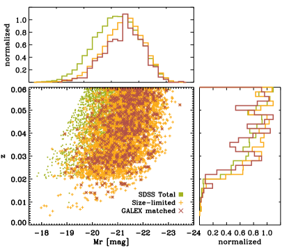
Figure 1.— Our sample of SDSS DR6 visually classified early-type galaxies at $0.00\leq z\leq 0.06$. Green points in the background indicate all early-type galaxies. Orange points represent the size-limited sample (a criterion imposed to obtain robust color gradients). We plot galaxies matched with GALEX as red points. We also plot histograms for M_r and z.

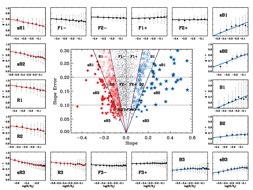
Figure 2.— Slope errors of early-tye galaxies versus $g-r$ radial slope – defined as d($g-r$)/d$\log$(R/R_e) – in the middle. The black solid lines indicate 0.5$\sigma$ (two sloped solid lines close to the vertical dotted line) and 1$\sigma$ confidence level lines, respectively. We select blue-cored galaxies that have steeper slope than the 0.5$\sigma$ confidence level line (blue stars). Red circles represent galaxies with negative $g-r$ gradients (red-cored) that have steeper slope than the 0.5$\sigma$ confidence level. Gradients from 0.5$\sigma$ and 1$\sigma$ level confidence are plotted as open and filled symbols, respectively. Bigger symbols represent steeper slopes. Sample plots of radial $g-r$ color gradients with different slope and slope errors are shown around the middle panel.

The Sloan Digital Sky Survey (SDSS) targets a large portion of the northern sky providing photometry in u, g, r, i and z bands. Furthermore, the SDSS spectroscopic survey includes virtually all extended objects with Petrosian magnitude r $<$ 17.77 that escape fiber collision problems (Strauss et al., 2002). We start by selecting all unsaturated galaxies with spectra in the redshift interval $0.00\leq z\leq 0.06$ and apply the apparent r band Petrosian magnitude cut of 17.50 to ensure the imaging quality suffices for the morphological classification of the sample. The SDSS photometry is given in the AB system (Oke & Gunn, 1983). However, it is known that the photometric zero points are slightly offset with respect to the AB standard. Therefore, we use the SDSS photometric flux calibration algorithm to obtain a calibrated magnitude and apply the offset between the SDSS system and the AB system (Bohlin, Dickinson & Calzetti, 2001). We also correct for Galactic extinction using the Schlegel et al. (1998) maps provided by the SDSS pipeline and apply a k-correction as described in Blanton & Roweis (2007). For galaxy luminosities, we used the SDSS petroMag, which is a good estimate of the total light, while the colors were derived from SDSS modelMags, which give a more reliable measure of unbiased colors regardless of any color gradients (Strauss et al., 2002).

Our next step involves the visual classification of the sample. We opted for a morphological classification instead of those based on color or concentration, as it reduces the bias that those methods have with respect to the presence of young stars. We make our initial selection based on the fracDev parameter, which is the weight of the deVaucouleur’s profile in the best composite (deVaucouleur’s + exponential) fit to the image in each band. We extract all galaxies which have fracDev $\geq$ 0.95 in g, r and i bands, following Yi et al. (2005) (see also Kaviraj et al., 2007; Schawinski et al., 2007a). On this sample, we perform visual inspection to exclude galaxies with spiral arms or distorted features. In addition, we exclude small galaxies to guarantee a reliable measurement of the radial color gradients (see §2.2). The final sample comprises a total of 5,002 early-type galaxies. Table 1 presents a summary of the selection criteria.

We cross-match the detections in the GALEX Medium Imaging Survey (MIS) with the SDSS early-type sample from 704 fields, with a 4 arcsec tolerance. In the case of multiple galaxy matches within a given matching radius, we select the UV source with the smallest angular separation from the position of the SDSS galaxy. We also de-redden the colors with respect to Galactic extinction using A_NUV = 8.741 $\times$ E(B$-$V) (Wyder et al., 2005) with the reddening maps from Schlegel et al. (1998) and apply a k-correction. In Figure 1, we plot all visually-inspected early-type galaxies as green points. The orange points correspond to the final size-limited sample (see §2.2 for details). Those galaxies in the final sample with a UV detection from GALEX are shown as red points. We also plot histograms for M_r and z.

Table 1Summary of sampling criteria

Criterion	Reason
r $<$ 17.50	Ensure photometric depth
0.00 $\leq$ z $\leq$ 0.06	Limit redshift for morphological
	classification
fracDevg,r,i $\geq$ 0.95	Robust morphological classification
Re $-$ RPSF $>$ 1.188”	Guarantee a reliable measurement of
	radial color gradients (having more
	than 3 fitting points between
	the PSF width and effective radius)

2.2. Measurement of color gradients

The SDSS provides the corrected frames (flat-fielded, sky-subtracted, and calibrated sub-images corrected for bad columns and cosmic rays) in five bands with $2046\times 1489$ pixels, sampled with $0.\arcsec 396\times 0.\arcsec 396$ pixels. Although the images are delivered pre-processed, we perform our own sky subtraction by measuring the sky level using the IDL “sky” Routine which adopts the technique from the DAOPHOT because the SDSS photometric pipeline tends to overestimate the sky background (von der Linden et al., 2007). We use the modal values for sky estimation.

We carry out the surface photometry of our sample of early-type galaxies in g and r bands (both of which are redward of the Balmer break) by measuring the surface brightness along elliptical annuli, implemented in the ELLIPSE task within the STSDAS ISOPHOTE package in IRAF (Image Reduction and Analysis Facility). We fixed the center of the isophotes to the center of the light distribution, and left the position angle (PA), ellipticity (e) and surface brightness ($\mu$) free as a function of radius. Ellipses were fit to the higher S/N r band image only, and then overlaid on the g band images so that the colors are extracted from the same regions.

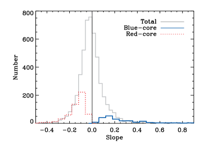
Figure 3.— The distribution of $g-r$ color gradients. From the total sample of 5,002 early-type galaxies, we select a subsample of 761 galaxies with significant color gradients. The gray histogram represents the entire sample of 5,002 galaxies (most of them showing a very small color gradient). The blue solid and red dotted histograms represent blue- and red-cored galaxies, respectively.

Table 2$g-r$ color gradients

Sample	mean(slopea)	median(slope)	mean($\Delta$slope)
Total (5,002)	-0.009	-0.017	0.21
$\Delta$slope${}^{b}<$ 0.1 (294)	-0.035	-0.036	0.08
$\Delta$slope $<$ 0.2 (1,555)	-0.026	-0.027	0.13
$\Delta$slope $<$ 0.3 (2,564)	-0.019	-0.023	0.18
Blue-coredc (216)	0.25	0.18	0.24
Strong blue-coredd (66)	0.41	0.41	0.25
Red-corede (545)	-0.14	-0.12	0.14

From the radial surface brightness profiles, we derive $g-r$ color gradients with a least-squares fit. The radial range of the fit is adjusted individually for each galaxy. The minimum radial coordinate of the fit is given by the FWHM of the point spread function (PSF), in order to minimize seeing effects. The PSF widths in the g and r bands are different. We select the worse case between them. Moreover, we use in the fit pixels out to an effective radius (R_e), because the data usually become noisy at larger radii. From this sample, we select those galaxies with more than 3 points (i.e. $\sim$1.188 arcsec) within the fitting range considered, to guarantee a reliable measurement of the radial color gradient – defined by its slope, $\equiv$ d($g-r$)/d$\log$(R/R_e). Additionally, we perform a Monte Carlo simulation comprising 10³ realizations adding noise to each point compatible with the observations, to assess the accuracy of the color gradients measured. We plot the uncertainty of the slope versus color gradient in the middle of Figure 2. The size of the symbols is proportional to the slope. We adopt a 0.5$\sigma$ confidence level (two sloped solid lines close to the vertical dotted line) to pick out galaxies that show statistically-significant color gradients. Using this criterion, we identify hereafter the blue-cored galaxies in Figure 2 as blue stars. We label galaxies with slope $<$ $-$0.5 $\times$ (slope error) as red-cored galaxies and show them as red circles thourghout this paper. Furthermore, open and filled symbols indicate the galaxies with slopes steeper than 0.5$\sigma$ and 1$\sigma$ confidence levels, respectively. Table 2 presents the mean values of the slope for different subsamples as shown in Figure 2. Note that galaxies with smaller uncertainties usually have negative slopes (red-cored). Furthermore, for a significant fraction of the sample the error estimates are rather large, a result of the shallow imaging of the SDSS survey.

We plot the distribution of $g-r$ color gradients in Figure 3. The gray line shows the histogram for a total of 5,002 galaxies. The blue solid and red dotted histograms correspond to blue- and red-cored galaxies, respectively. The overall fraction of blue- and red-cored galaxies within our criterion is roughly 4 per cent (216/5,002) and 11 per cent (545/5,002), respectively. We note that roughly 30 per cent of the galaxies with detectable color gradients have positive values (i.e. blue-cored). In other words, more early-type galaxies tend to have negative color gradients (i.e. red-cored).

To measure the line strengths, we use the GANDALF (Gas AND Absorption Line Fitting) package (Sarzi et al., 2006). It is important to remove the contribution from emission lines in order to track the true values of absorption from the underlying stellar populations. Contamination due to emission lines from extended regions of ionized gas exists in roughly 75 per cent of early-type galaxies. The GANDALF measurements, such as standard Lick absorption line indices, emission line strengths and velocity dispersions of the SDSS galaxies are described in detail in Oh et al. (in preparation).

3. Results

3.1. Color-magnitude relation

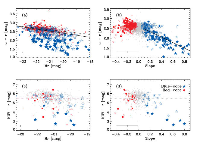
Figure 4.— Gray dots in the background represent all galaxies. We plot blue-cored and red-cored galaxies with blue stars and red circles, respectively. A typical error bar is shown as comparison. (a) $u-r$ vs. M_r color-magnitude relation. Black solid and dotted line indicate the least-square fit to the total sample and only to the red-cored galaxies, respectively. (b) $u-r$ color vs. $g-r$ radial slope. The black line indicates the least-square fit of blue-cored galaxies. (c) NUV$-$r color-magnitude relation. (d) NUV$-$r color vs. $g-r$ slope. The symbols are the same as Figure 2.

The color-magnitude relation is widely used to study the star formation history of early-type galaxies (see e.g. Bower, Lucey & Ellis, 1992b; Stanford et al., 1998; Ferreras et al., 1999). The correlation between metallicity and luminosity is the main reason of this relation (Kodama & Arimoto, 1997). The optical color-magnitude relation of early-type galaxies reveals a small scatter around the mean relation (e.g. Bower, Lucey & Ellis 1992; Ellis et al. 1997; van Dokkum et al. 2000). Figure 4(a) shows the $u-r$ color-magnitude relation. We note that the $u$ band is particularly sensitive to the presence of young stellar populations. The figure also shows the least-squares fit to the whole sample (solid) and only to the red-cored galaxies (dotted). The gray points, blue stars and red circles indicate the whole sample, blue-cored and red-cored galaxies, respectively. A cursory inspection of this diagram shows that most blue-cored galaxies are located in the blue cloud, while red-cored galaxies reside in the red sequence, in agreement with recent studies of early-type galaxies at moderate redshift (Ferreras et al., 2009). It should also be noted that a non-negligible fraction of the scatter in the optical color magnitude relation is due to blue-cored galaxies.

We also show integrated $u-r$ color versus the slope of the $g-r$ color gradient in Figure 4(b). It reveals that a strong correlation is present amongst the blue-cored galaxies, with a correlation coefficient $r=$ 0.76. This implies that whenever star formation is present in early-type galaxies, it is mostly concentrated in the central regions, at least within the effective radius. We recall however that some galaxies show significantly bluer $u-r$ colors even though they have shallower slopes. These galaxies show that the $g-r$ color is significantly bluer out to at least the effective radius, suggesting spatially extended star formation. Meanwhile, we note that some red-cored galaxies with steep slopes show slightly blue $u-r$ colors. In this case, the presence of off-centered young stellar populations can explain both the bluer integrated color and the steep color gradient.

The NUV color-magnitude relation (see, e.g., Yi et al. 2005; Kaviraj et al. 2007; Schawinski et al. 2007a) is a particularly efficient tool for tracking recent star formation, owing to its high sensitivity to young stellar populations. In Figure 4(c, d), we show the NUV$-$r color-magnitude relation and NUV$-$r color versus slope in the $g-r$ radial gradient. The empirical threshold at NUV$-$r $<$ 5.5 of Yi et al. (2005) (based on NGC 4552) to indicate recent star formation is shown as a dashed line. We find that blue-cored galaxies with steep slopes (filled stars) reside almost exclusively below NUV$-$r $\sim 5.5$, supporting our findings that most of blue-cored galaxies have undergone recent star formation, while red-cored galaxies are relatively red in the NUV. Interestingly, all blue-cored galaxies show blue NUV$-$optical colors but the converse is not always true. We note that there are some red-cored galaxies with NUV$-$r $<$ 5.5. This indicates that some early-type galaxies have steep negative color gradients because of the presence of young stars in the outer regions. For example, NGC 2974 – classified as an early-type galaxy in the optical – shows blue UV$-$optical colors at large radii (Jeong et al., 2007). The UV bright outer ring observed in this galaxy is related to a bar, demonstrating that recent star formation can be found in the form of a ring in the outer part of an early-type galaxy.

3.2. Velocity dispersion

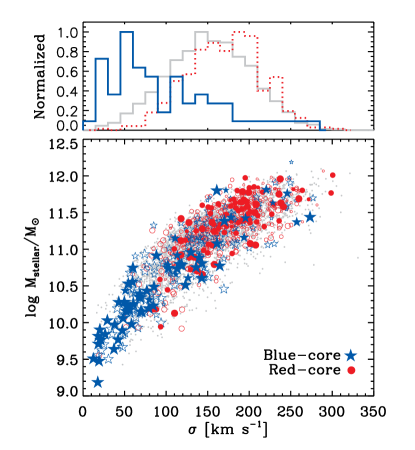
Figure 5.— Top: The distribution of velocity dispersion for our early-type galaxies. The gray histogram represents the total sample. Blue solid and red dotted histograms represent blue-cored and red-cored galaxies, respectively. Bottom: Stellar mass of early-type galaxies versus velocity dispersion. Blue-cored galaxies tend to have lower stellar velocity dispersion, while red-cored galaxies are more massive. The symbols are the same as in Figure 2.

The stellar velocity dispersion is correlated with a galaxy mass (e.g. Faber & Jackson, 1976). Aperture corrections are applied to the observed velocity dispersion due to the fact that the fixed-diameter fibers sample larger portions of galaxies at larger distance, systematically underestimating the true velocity dispersion (Bernardi et al., 2002; Kauffmann et al., 2003; Tremonti et al., 2004; Kewley et al., 2005; Kewley & Ellison, 2008). The applied aperture corrections follow Cappellari et al. (2006), namely:

$$\rm\sigma_{\rm corr}=(\frac{R_{\rm fiber}}{R_{e}})^{0.066\pm 0.035}\sigma_{\rm fiber},$$ (1)

where R_fiber is 1.5 arcsec and R_e is the effective radius.

We show the distribution of velocity dispersions for our sample of early-type galaxies in the top panel of Figure 5. We find that red-cored galaxies (red dotted) are relatively massive compared to average early-type galaxies (gray) while blue-cored galaxies (blue solid) tend to have lower stellar velocity dispersion, once more in agreement with studies at moderate redshift (e.g. Ferreras et al., 2009; Kannappan et al., 2009). In the bottom panel of Figure 5, we also plot the velocity dispersion versus stellar mass. The stellar masses were derived by fitting the $u,g,r,i$ and $z$ SDSS photometry using a two-burst scenario (e.g. Ferreras & Silk, 2000; Kaviraj et al., 2007; Schawinski et al., 2007b) with the stellar models of Maraston (2005). Variable parameters include the age and mass-fraction of the young burst, the age of the old burst and the amount of dust extinction following the Calzetti et al. (2000) law. We measure stellar masses by minimizing the $\chi^{2}$ statistic. It is interesting to notice that the transition between blue- and red-cored galaxies occurs at around $M_{s}\sim 0.5-1\times 10^{10}$M_⊙, which is the threshold below which the stellar populations of elliptical galaxies become younger (Rogers et al., 2008).

3.3. H$\beta$ absorption line

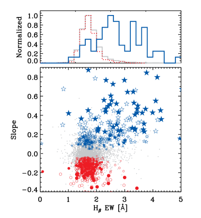
Figure 6.— Top: The distribution of H$\beta$ absorption line strength for our early-type galaxies. The gray histogram represents the total sample, blue solid histogram represents blue-cored galaxies and red dotted histogram represents red-cored galaxies. Bottom: $g-r$ radial slope of early-type galaxies versus H$\beta$ absorption line strength. Blue-cored galaxies show stronger H$\beta$ absorption than red-cored galaxies. The symbols are the same as in Figure 2.

The presence of strong Balmer absorption lines betray the presence of main sequence stars formed in the past $\sim 1$ Gyr. In Figure 6, we show in the top panel the distribution of the equivalent width (EW) of H$\beta$ for our early-type galaxies. The distribution of H$\beta$ EWs for red-cored galaxies (red dotted) is similar to that of the whole sample (gray). Interestingly, blue-cored galaxies (blue solid) have a distribution of H$\beta$ strengths that peaks at a roughly 1.5 Å higher EW than the general sample. This is more evidence towards recent star formation in blue-cored galaxies. In the bottom panel, we show a trend between the H$\beta$ EW and the $g-r$ color gradient. We note that blue-cored galaxies with steeper slopes tend to show enhanced H$\beta$ line strengths, which would imply that young stellar populations in the central region are responsible for the color gradients.

Table 3Spectral line Classification Results

Classification		Total	strong blue-cored1	blue-cored	red-cored
Number		5002 (100%)	66 (100%)	216 (100%)	545 (100%)
Strong emission2		549 (10.97%)	44 (66.67%)	85 (39.35%)	60 (11.01%)
	Starforming…	185 (3.70%)	29 (43.94%)	47 (21.76%)	6 (1.01%)
	Transition……	176 (3.52%)	5 (7.58%)	12 (5.55%)	19 (3.48%)
	Seyfert………..	80 (1.60%)	8 (12.12%)	15 (6.94%)	3 (0.55%)
	LINER………..	107 (2.14%)	2 (3.03%)	11 (5.09%)	32 (5.87%)
Strong H$\beta$ absorption3		1020 (20.39%)	53 (80.30%)	127 (58.79%)	79 (14.49%)
Quiescent4		3836 (76.69%)	7 (10.61%)	75 (34.72%)	421 (77.25%)

3.4. Emission line diagnostics

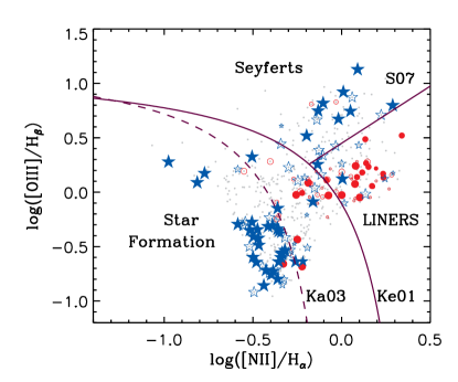
Figure 7.— The emission line diagnostic diagram for our sample (Baldwin, Phillips, & Terlevich, 1981). We only plot galaxies where [N II], H$\alpha$, [O III] and H$\beta$ lines are detected with S/N $>$ 3. The curve labeled Ka03 is the empirical purely star-forming llimit of Kauffmann et al. (2003), while the curve labeled Ke01 represents the theoretical maximum starburst model from (Kewley et al., 2001). All galaxies between the Ka03 and the Ke01 are transition systems that they do have emission lines with contributions from both star-formation and AGN. The line from S07 (Schawinski et al., 2007b) divides Seyferts and LINERS. The symbols are the same as Figure 2.

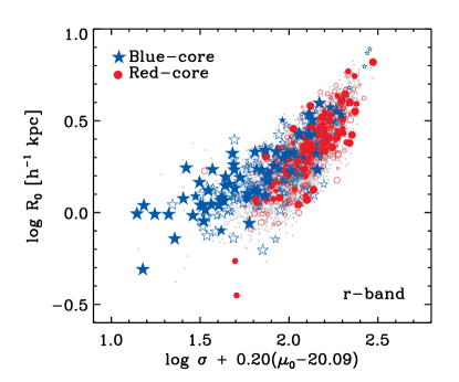
Figure 8.— The Fundamental Plane of early-type galaxies. blue-cored and red-cored galaxies are marked with blue stars and red circles, respectively. Gray points in the background indicate all early-type galaxies. There are indications that red- and blue-cored galaxies may lie on different planes. The symbols are the same as in Figure 2.

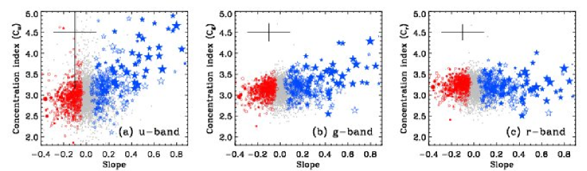
Figure 9.— The u, g and r band concentration indices of early-type galaxies as a function of $g-r$ slope. Gray dots in the background indicate the total sample of visually classified early-type galaxies. The symbols are the same as Figure 2, but the symbol size represents H$\beta$ absorption line strength. The typical 1-sigma error in the measurements is shown in each panel. The slope errors are measured in this study, and the concentration index errors are adopted from the SDSS database.

Emission-line diagnostic diagrams are useful tools to distinguish between star formation and AGN activity. The BPT diagram (Baldwin, Phillips, & Terlevich, 1981) allows the classification of galaxies with (narrow) emission lines into star-forming galaxies and AGN. AGN are also split into Seyfert II AGN and LINERs (Low Ionization Nuclear Emission Line Region). In Figure 7, we plot the BPT diagram using the emission line ratios [O III]/H$\beta$ and [N II]/H$\alpha$. Only galaxies with a signal-to-noise (S/N) above 3 (Kauffmann et al., 2003) in all four lines are shown in the diagram. We use the demarcation line by Kauffmann et al. (2003) (dashed curve) to separate star-forming galaxies. The remaining galaxies are divided into AGN and transition region. The latter correspond to a blend of star-forming and AGN galaxies, and are located between the empirical line of Kauffmann et al. (2003) and the theoretical maximum starburst model of Kewley et al. (2001) (solid curve). AGN are subclassified into Seyferts and LINERs as shown by the straight solid line (Schawinski et al., 2007b).

In Table 3, we show the results of the spectral line classification. Most early-type galaxies are virtually free of emission lines ($\sim$89 per cent; that is, total(100) minus strong emission(10.97)). Twenty three per cent of total early-type galaxies (that is, total(100) minus quiescent(76.69)) show significant emission lines (S/N $>$ 3 in all four BPT lines) or strong H$\beta$ absorption lines ($EW(H\beta)>2$). We find that about 65 per cent (that is, total(100) minus quiescent(34.72)) of blue-cored galaxies show strong H$\beta$ absorption and/or emission lines. Most of the emission line ratios are consistent with ongoing star formation. Only 10 per cent (quiescent; 10.61 per cent) of blue-cored galaxies with slopes steeper than the 1$\sigma$ confidence level (i.e. strong positive color gradient galaxies) show neither emission nor strong Balmer absorption lines. Interestingly, some blue-cored galaxies are classified as Seyferts. Therefore, we note that blue-cored galaxies are mainly due to centrally concentrated star formation and a smaller fraction could be associated with Seyfert activity. Most red-cored galaxies, on the other hand, are classified as quiescent (78.98 per cent). If red cores show emission lines, most of their emission line ratios are consistent with LINER AGN. red-cored galaxies appear $not$ to be host to active star formation or powerful AGN.

3.5. Fundamental Plane

Early-type galaxies exhibit a scaling relation between the effective radius $R_{\rm e}$, the effective mean surface brightness $\mu_{e}$ and central velocity dispersion $\sigma$ (i.e. the Fundamental Plane, FP, Dressler et al. 1987; Djorgovski & Davis 1987). We compare here the location of blue-cored and red-cored galaxies on the FP. In order to construct the fundamental plane of our early-type galaxies, we have to apply a number of corrections as follows. We convert an elliptical aperture to an effective circular radius (Bernardi et al., 2003) and apply a k-correction and the cosmological dimming effect:

$$\rm R_{e}\equiv\sqrt{b/a}R_{dev},$$ (2)

$$\rm\mu=m_{dev}+2.5log(2\pi(R_{e})^{2})-K(z)-10log(z+1),$$ (3)

where b/a is the ratio of the minor and major axes, $R_{\rm dev}$ and $m_{\rm dev}$ are the effective radius and apparent magnitude, respectively, from the de Vaucouleurs fit (de Vaucouleurs, 1948).

We show in Figure 8 the FP of the total sample (gray), blue-cored galaxies (blue stars) and red-cored galaxies (red circles). Red- and blue-cored galaxies appear to lie on different planes. A more detailed analysis is on the way. We will discuss this discrepancy via stellar population modelling in §4.2.

3.6. Concentration index

The concentration index is often used as a quantitative measure of galaxy morphology (see e.g. Morgan & Mayall, 1957; Conselice, 2006) and is a useful tool because the surface brightness distribution of a galaxy depends strongly on its formation history. The concentration index, C, is defined as the ratio between R₉₀ and R₅₀ from the SDSS pipeline parameters, which are the radii that encompass 90 and 50 per cent, respectively, of the Petrosian flux, namely:

$$\rm C_{x}=\frac{R_{x90}}{R_{x50}},$$ (4)

where x =u, g, r  labels the SDSS band used to determine the concentration (Stoughton et al., 2002). After unresolved sources (which just result in a PSF), early-type galaxies are the most concentrated systems with C${}_{r}>2.6$ (see Figure 1 of Ferreras et al., 2005).

In Figure 9, we show the u, g and r band concentration indices versus the slope of $g-r$ color for our sample of early-type galaxies. The color code for the symbol is the same as in Figure 2. The size of the symbols is proportional to the H$\beta$ line strength. The right panel indicates that blue-cored and red-cored galaxies show similar concentration index in the r band. However, the other panels show that a significant fraction of blue-cored galaxies are more concentrated in u and g bands, while there is a tendency for red-cored galaxies to be less concentrated, although examples of galaxies showing the opposite behavior can also be identified. We note that the most concentrated blue-cored galaxies in u band tend to also show strong H$\beta$ absorption lines, indicating large fractions of young populations in the center. This difference as well as the increase in scatter are naturally explained by the different sensitivity of the passbands to young stars.

3.7. Environment

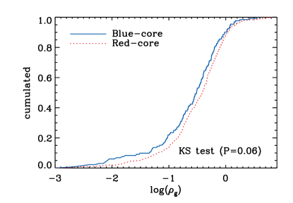
Figure 10.— Cumulative distribution of the local density log($\rho_{g}$). In order to minimize a selection bias with stellar mass, this figure shows both blue-cored and red-cored galaxies in the same stellar mass bin (10.5 $<$ log(M/M_⨀) $<$ 12). The KS test discriminates between these two distributions at a 95% confidence level. blue-cored galaxies tend to prefer slightly lower density regions compared to red-cored galaxies.

We find evidence that a large fraction of blue-core galaxies have undergone recent star formation from H$\beta$ absorption line strengths and emission line diagnostics. We now address the possible cause of this recent star formation in early-type galaxies. One possible scenario involves galaxy mergers and interactions. If galaxies experience merging events involving gas-rich late-type galaxies, it might result in enhanced star formation during the encounter. We investigate this possibility by looking at environment and also by checking the nature and location of the nearest neighbor.

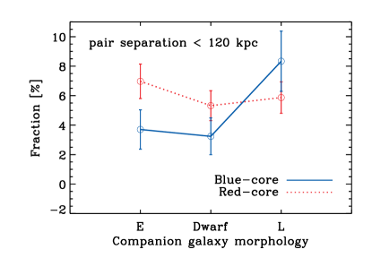
Figure 11.— Fraction of pair galaxies with respect to (visually classified) morphology. The morphologies of pair galaxies are divided into three types: early-type galaxy (E), dwarf galaxy (Dwarf) and late-type galaxy (L). Blue-cored galaxies appear more are likely to have a late-type companion.

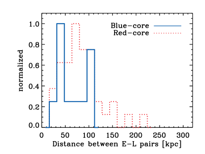
Figure 12.— The distribution of separation in close pairs (within 300 kpc) comprising an early- and a late-type galaxy. Pairs with a blue-cored galaxy are found at shorter separations with respect to pairs with a red-cored galaxy.

Figure 10 shows the cumulative distribution of the local density parameter $\rho_{g}$ defined by Schawinski et al. (2007a) (see also Yoon et al., 2008). This density parameter ($\rho_{g}$) represents a weighted local number density, and is obtained by counting all neighbors within 2 Mpc with a Gaussian-weighting scheme. In order to avoid selection bias with respect to mass, we limit both blue-cored and red-cored galaxies to the same stellar mass range between 10.5 $<$ log(M/M_⨀) $<$ 12. We perform the Kolmogorov-Smirnov test (KS test) and find that blue-cored and red-cored galaxies are not consistent with being drawn from the same parent population at the 95 per cent confidence level. These two cumulative distributions of $\rho_{g}$ show that blue-cored galaxies prefer lower density environments compared to red-cored galaxies. However, this may also come from the fact that more massive galaxies reside in denser regions. For a narrower mass bin, we find less clear density dependence. But we had to use such as large mass range for this statistical test because the number of blue-cored galaxies in our sample is limited. We would need a much larger sample to break the mass-density degeneracy.

We also consider the nearest neighbor galaxies and their morphology. Two galaxies are considered to be in a close pair if r_p $<$ 120 kpc (where $r_{\rm p}$ means projected physical separation) and $\Delta$z $<$ 0.001. We show the fraction of galaxies in close pairs in Table 4. Radial color gradients seem insensitive to pair galaxy fraction. However, this analysis is hampered by projection effects that can mimic true pairs which are more serious in denser regions.

If the recent star formation in the central region of blue-cored galaxies is caused by gas inflows from a neighboring galaxy, one might wonder whether the morphology of a companion galaxy – which correlates with gas fraction – could affect color gradients. To test this point, we perform visual classification of the companion galaxies. The morphology of the companion galaxies are classified into three types: early-type (E), dwarf (Dwarf) and late-type (L). Figure 11 shows the fraction of pair galaxies with respect to the companion morphology. Taken at face value, blue-cored galaxies have more late-type companions than red-cored galaxies.

Figure 12 shows the distribution of pair separation in systems comprising an early- and a late-type galaxy. We find that pairs with a blue-cored galaxy have smaller separations than those with a red-cored galaxy, in agreement with the picture that a nearby, gas-rich late-type galaxy can contribute to the onset of residual star formation. However, we should emphasize here that most (92 per cent) of the blue-cored galaxies in our sample do not have a late-type companion. The presence of a late-type companion may affect the star formation of the galaxy in question, but not all star-forming early types are caused by the presence of a late-type companion. Hence, other mechanisms (such as minor mergers with nearby gas rich dwarf galaxies or even gas clouds) should be invoked to explain the general trend.

Table 4Pair galaxy fraction

Classification	Fraction (r${}_{p}<$ 120 kpc)
Total	764/5002 (15.27%)
blue-cored	45/262 (17.18%)
red-cored	120/647 (18.54%)

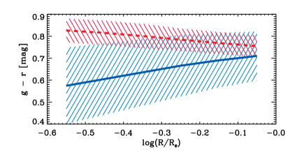
Figure 13.— The mean radial $g-r$ color gradients of blue-cored (blue solid) and red-cored (red dotted) galaxies. The shading corresponds to the scatter within the sample, given at a 1$\sigma$ confidence level.

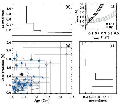
Figure 14.— The normalized likelihood distribution in age and mass fraction for the young stellar component. (a) The star symbols represent the best fits to the blue-cored galaxies (as classified in Figure 2) along with error bars in grey. Only those with $\chi_{\rm red}^{2}<3$ are shown here. The contour gives the 1$\sigma$ confidence level from a Monte Carlo simulation (see text for details). (b) Normalized age distribution. (c) Normalized mass fraction of the young stellar component. (d) A typical $\chi^{2}$ marginalization for a galaxy. This particular case is for the circled galaxy in (a).

4. Discussion

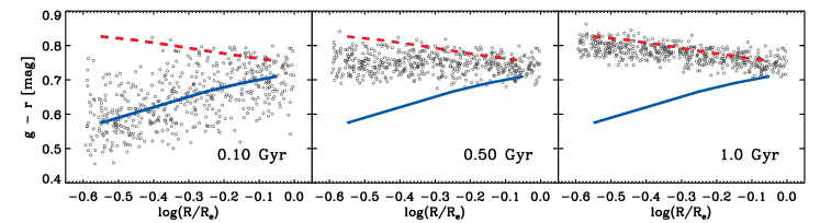
Figure 15.— The evolution of the color gradient for blue-cored galaxies. The blue solid and red dotted lines represent the mean radial $g-r$ color gradients of blue-cored and red-cored galaxies, respectively. The open circles correspond to models using the observations of red-cored and blue-cored galaxies as constraints on a two-burst scenario (see text for details). As the populations age (from left to right), the blue-cored galaxy transforms into a red-cored galaxy.

Figure 16.— Evolution of slope obtained from the probability distribution in the age and mass fraction of the young component. We show how the slope evolves for various possible choices of the young stellar mass fraction. We choose mass fractions from the peak of the probability distribution (solid), or at the 1$\sigma$ (dotted), 2$\sigma$ (dashed) and 3$\sigma$ (dot-dashed) confidence levels. The slope of blue-cored galaxies decreases rapidly from positive to negative in about 1.5 Gyr after the star formation episode.

4.1. Age and mass fraction of young stars

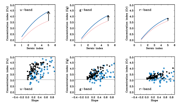
Figure 17.— Top: Concentration indicies of u, g and r band as a function of S$\acute{e}$rsic index. The red dotted line represents the concentration index assuming a purely old population. The blue solid line shows the effect of a centrally concentrated young population on each passband. Bottom: Concentration indicies versus slope. The stars represents observed blue-cored galaxies and the squares show the results from the modelling (see text for details). The gray horizontal line marks the mean concentration index of the total sample in each passband.

The aim of this section is to quantify the amount of recent star formation in our sample. In order to study the radial distribution of young stars, we construct the mean $g-r$ radial color gradient of the sample, shown in Figure 13. The dotted and solid lines indicate red-cored and blue-cored galaxies, respectively. The shading in each case represents the 1$\sigma$ confidence level. Color gradients in early-type galaxies are usually a result of the underlying stellar populations, mainly in age and metallicity. It is difficult, however, to distinguish the effects of a small change in age from those of a small change in metallicity. Most red-cored galaxies, however, tend to show overall red $u-r$ colors (see §3.1) and weak H$\beta$ line strengths (see §3.3), suggesting an old population. Therefore, we consider the negative slopes of red-cored galaxies as a result of a simple metallicity gradient and assume that blue-cored galaxies have the same metallicity gradient. This assumption is also motivated by the lack of evolution in the color gradient of red-cored galaxies with redshift (Ferreras et al., 2005, 2009).

To calculate the characteristic metallicity of each region in the galaxy, we assume a single uniform age of 12 Gyr but change the metallicity distribution until it matches the observed $g-r$ color. The base model in this study are those of Yi (2003) which are specialized for old populations. Since those models do not cover ages younger than 1 Gyr, however, we combine them with the models of Bruzual & Charlot (2003). According to the models, the central region in red-cored galaxies has a metallicity distribution with a peak around the solar value, while at the effective radius the peak decreases to half the solar.

We consider a two-stage star formation history to determine the age and mass fraction of the young stellar component of blue-cored galaxies. This model combines an old and a young stellar population (Ferreras & Silk, 2000; Kaviraj et al., 2007; Schawinski et al., 2007b). The old population has a fixed age of 12 Gyr with a metallicity gradient determined from the mean radial color gradient of red-cored galaxies. The young component has the solar metallicity and is allowed to vary in age ($0.01\leq t_{young}\leq$10 Gyr) and mass fraction ($10^{-4}\leq f_{young}\leq 1$). To constrain these two parameters, we fit the observed $g-r$ color and H$\beta$ EW to models and compute the associated $\chi^{2}$ statistic to obtain a probability distribution of the age and mass fraction of the young stellar population. We further perform a Monte Carlo simulation with $10^{3}$ realizations to explore the parameter space for minima and the associated errors around them. The best fit and confidence levels are shown in Figure 14(a) and also in the accompanying histograms (b and c). In panel (d) we show the $\chi^{2}$ minimization performed on a sample galaxy, circled star in (a). These clearly show that young ($\sim 10^{2}$ Myr old) stellar populations are present in the central region and the stellar mass fraction of the young component reaches up to a couple of per cent.

By evolving the young component in time, we can derive the evolution of the slope. Figure 15 shows the evolution of model blue-cored galaxies, assuming the mean properties and scatters for the young population derived here. The color gradients observed suggest that this young component should have a decreasing contribution with increasing radius. Hence, we choose a central value for the mass fraction in young stars of 0.7 per cent and decrease this mass fraction outward in a manner that reproduces the observed $g-r$ profiles. Its mean age is assumed to be 100 Myr to begin with, and we monitor the color gradient as time goes on. The solid and dashed lines represent the mean radial $g-r$ color gradients of blue-cored and red-cored galaxies, respectively. The color gradients caused by the young population revert to the fiducial values of red-cored galaxies after about 1 Gyr, as expected given the small fractions in young stars. In Figure 16 we show the evolution of the change in slope with respect to different values of the mass fraction in young stars. We choose four different cases based on the probability distribution of the modeling (see Figure 14). We consider the peak of the probability distribution (0.7 per cent, solid), and the 1$\sigma$ (1.8 per cent, dotted), 2$\sigma$ (3.9 per cent, dashed), and 3$\sigma$ (5.7 per cent, dot-dashed) confidence levels. The slope of the blue-cored galaxies changes rapidly from positive to negative. The positive gradients in early-type galaxies must be transient features that are visible only for $\sim$0.5 – $\sim$1.3 billion years or so after a centrally-concentrated star formation episode (see figure 8 of Ferreras et al., 2009).

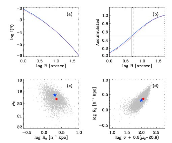
Figure 18.— (a) The surface brightness distribution. The dotted line represents the intensity profile assuming a purely old population. The intensity profile is normalized to I(0). The solid line shows the combined light profile of the old and young populations. (b) Cumulative light profile. Dotted and solid lines represent the underlying old population and the combined model, respectively. The vertical lines represent the effective radius of each profile. (c) The effect of a centrally concentrated young population on the Kormendy relation. Red circle and blue star represent old and total (old plus young) model, respectively. The gray dots in the background indicate all observed early-type galaxies. (d) The effect of a centrally-concentrated young population on the FP. Symbols are the same as in (c).

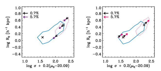
Figure 19.— The effect of a centrally concentrated episode of star formation on the FP. Blue solid and red dotted lines delimit the observed FP (shown at the 1$\sigma$ confidence level) for blue-cored and red-cored galaxies, respectively. The vectors show the contribution of a 100 Myr young components with a mass fraction of 0.7% or 5.7%. Left: Effect of a young component on red-cored galaxies. Right: Effect of ageing of the young component of blue-cored galaxies.

4.2. The effect of young stars

We now discuss the effect of the young stellar populations on the concentration index and the FP. To explore the effect of young stars on these properties, we compute the change of the surface brightness distribution of a galaxy due to recent star formation in the central region. We start from the S$\acute{e}$rsic profile:

$$I(R)=I(0)\exp[-k(R/R_{e})^{1/n}]$$ (5)

For $n\geq 1$, $k$ satisfies the relation $k=2n-0.324$ (Ciotti, 1991).

We assume that the intensity profile of the underlying old population has the metallicity gradient constrained by the color gradient and that the young stellar populations are more centrally concentrated to satisfy the observed positive color gradients. A model effective radius of 5 arcsec is chosen for this exercise. We construct the total light profile as the superposition of the surface brightness profile for the old and young populations. This profile allows us to quantify the effect of a young component on the effective radius, mean surface brightness or concentration index.

4.2.1 Concentration index

The concentration index is a useful tool because the surface brightness distribution of a galaxy depends strongly on its formation history. Star formation, mergers and accretion events might affect the surface brightness distribution by rearranging the stellar components in the progenitors as well as by forming new stars in geographically biased ways. For example, if star formation is triggered towards the center, the concentration index will increase.

Figure 17 shows the concentration index of the old (dotted) and the mixed (solid) populations. The top panels of Figure 17 show that the strongest effect is on the concentration measured in the u band because of its highest sensitivity to young stars. We also show the increase of the concentration index as a function of slope in the bottom panels. The horizontal line indicates the mean concentration index for the total sample in each passband. Using the estimated best fit age and mass fraction of the young stellar component of blue-cored galaxies (see §4.1), we compare our models (black squares) with observations (stars). The concentration index in the model shows a clear correlation with the radial color gradient slope. The correlation is stronger for shorter wavelengths. The match seems poor for the $u$ band. This is probably because of the inaccuracy of our model assumptions. We assumed that recent star formation occurred only in the central region, from center to effective radius. However, the SDSS concentration indices are measured from the whole radial range. If the residual star formation extends outside the effective radius, it would lower our model concentration index to match the data better. But such a detailed modeling is beyond the scope of this investigation. Despite the simplicity of the model considered here, we successfully match the observed concentration indices in various bandpasses.

4.2.2 Fundamental plane

In order to examine the effect of the young population on the FP, we calculate the change of the effective radius and the mean surface brightness due to recent star formation in the central region. We assume that the surface brightness distribution of a red-cored early-type galaxy follows a de Vaucouleurs’ profile (i.e. Sersic index $n=$ 4).

In Figure 18(a), we show the intensity profile of the underlying old population (dotted) and the combined profile (solid). We show the cumulative luminosity profiles in Figure 18(b). A population with young stars at the center tends to have a smaller effective radius and a brighter mean surface brightness, as shown for the Kormendy relation in Figure 18(c). In order to study the effect of this centrally concentrated young population on the FP, we compare our models with observations, as shown in Figure 18(d). This suggests that although the models predict a significant offset in the Kormendy relation, the effect is more subtle on the FP. Hence, the clear difference between the observed blue- and red-cored galaxies on the FP (Figure 8) seems beyond what can be modeled by a simple addition of young stars. Instead, one needs to consider that blue-cored galaxies indeed have on average lower velocity dispersions than the general sample.

To further illustrate this point, Figure 19 shows the effect of centrally concentrated recent star formation on the FP. The solid and dotted contour lines delimit the region occupied by the FP for blue-cored and red-cored galaxies, respectively. The black and purple/pink arrows correspond to the presence of 0.7 or 5.7 per cent of a 100 Myr population at the center. The left panel considers what would happen if this young component is added to the population of red cores. On the right panel, we consider the fading of this young component in blue-cored galaxies, as the galaxies age. In both cases we find that blue/red-cored galaxies belong to different distributions, separated by velocity dispersion (or stellar mass). One can clearly see that although the most massive blue-cored galaxies could be explained by a recent episode of star formation (comprising 6 per cent of its stellar mass content, which is hardly unjustifiable), for the majority of (low mass) blue-cored early-type galaxies, one must consider that they correspond to systems with markedly lower velocity dispersion than red-cored galaxies.

5. Summary

We present radial $g-r$ color gradients of visually classified early-type galaxies at $0.00\leq z\leq 0.06$ selected from Data Release 6 of the Sloan Digital Sky Survey. Due to the shallow exposure of DR6 color gradients are difficult to measure in the bulk of the sample. The brightest galaxies exhibit a negative color gradient (centrally redder) as expected for their observed radial metallicity variations. However, a significant fraction – roughly 30 per cent which might depend on data selection strategy – features blue cores (positive color gradients). Evidence is presented, suggesting that these blue-cored galaxies have undergone a recent episode of star formation that is centrally concentrated. Most are blue also in terms of integrated $u-r$ colors and show strong central H$\beta$ absorption line strengths and/or emission ratios that are consistent with star forming populations. Combining SDSS and GALEX UV photometry, we find that all blue-cored galaxies show blue UV$-$optical colors. They also tend to have a lower stellar velocity dispersion. We investigate their environmental dependence and star formation properties. Blue-cored galaxies exhibit a tendency to live in lower density environments compared to red-cored galaxies and, if found in close pairs, have a preference for a late-type companion. On the other hand, red-cored galaxies, which are relatively massive, are located on the red sequence as shown in the integrated $u-r$ color-magnitude relation, and those with emission lines reside in the LINER region of a BPT diagram.

Based on a simple model that overlays a young stellar component over an old population, our sample gives a mass fraction in young stars below 2 per cent with age 100$-$800 Myr in the central regions of blue-cored galaxies. Furthermore, these positive color gradients in early-type galaxies are visible only for $\sim$0.5 – $\sim$1.3 billion years after a star formation event. Although this centrally located star formation episode can decrease the effective radius and increase the mean surface brightness, the FP of the (majority of) low mass blue-cored galaxies cannot be reproduced by any amount of recent star formation on a red-cored galaxy. Instead, they require a lower velocity dispersion, i.e. blue-cored and red-cored early-type galaxies are, perhaps fundamentally, different populations, mainly split with respect to stellar mass or velocity dispersion.

From the perspective of our investigation on the optical color gradients, we conclude that star-forming early types are not simply the star-forming counterparts of the quiescent ones. While many parameters are connected to each other in degenerate manners, the most important role seems to be played by galaxy mass. This star-formation dichotomy (between the star-forming and quiescent early types) is consistent with that of Schawinski et al. (2006) and also with the kinematic dichotomy previously addressed (e.g. Davies et al., 1983; Bender, 1988; Kormendy & Bender, 1996; Faber et al., 1997; Rest et al., 2001; Lauer et al., 2007; Kimm & Yi, 2007). Recent theoretical models (e.g. Khochfar & Silk, 2009) explain the star-forming dichotomy in connection with the kinematic dichotomy through distinct merging histories by mass. More massive early types are interpreted as results of equal-mass dry mergers. This is compatible to the axis ratio distribution analysis of Kimm & Yi (2007). On the other hand, small early types are suggested to be a product of early-type and late-type merger, in which case the cold gas from the late-type component would linger in the merger remnant and get used for residual star formation. Kaviraj et al. (2009) further point out that it was more likely minor mergers than major ones that was involved in the formation of low-mass early types exhibiting signs of residual star formation. All these works together seem to suggest a coherent picture for the formation of early-type galaxies.

References

- Adelman-McCarthy et al. (2008) Adelman-McCarthy, J. K., et al. 2008, ApJS, 175, 297
- Baldwin, Phillips, & Terlevich (1981) Baldwin, J. A., Phillips, M. M., Terlevich, R. 1981, PASP, 93, 5
- Bamford et al. (2009) Bamford, S. P., et al. 2009, MNRAS, 393, 1324
- Bartholomew et al. (2001) Bartholomew, L. j., Rose, J. A., & Gaba, A. E. 2001, AJ, 122, 2913
- Bender (1988) Bender, R. 1988, A&A, 193, L7
- Bernardi et al. (2002) Bernardi, M., et al. 2002, AJ, 123, 2159
- Bernardi et al. (2003) Bernardi, M., et al. 2003, AJ, 125, 1817
- Blake et al. (2004) Blake, C., et al. 2004, MNRAS, 355, 713
- Blanton & Roweis (2007) Blanton, M. R. & Roweis, S. 2007, AJ, 133, 734
- Bohlin, Dickinson & Calzetti (2001) Bohlin, R. C., Dickinson, M. E., & Calzetti, D. 2001, AJ, 122, 2118
- Boroson et al. (1983) Boroson, T. A., Thompson, I. B., & Shectman, S. A. 1983, AJ, 88, 1707
- Bower, Lucey & Ellis (1992) Bower, R. G., Lucey, J. R., Ellips, R. S. 1992, MNRAS, 254, 589
- Bower, Lucey & Ellis (1992b) Bower, R. G., Lucey, J. R., Ellips, R. S. 1992b, MNRAS, 254, 601
- Bruzual & Charlot (2003) Bruzual, G., & Charlot, S. 2003, MNRAS, 344, 1000
- Calzetti et al. (2000) Calzetti, D., Armus, L., Bohlin, R. C., Kinney, A. L., Koornneef, J., Storchi-Bergmann, T. 2000, ApJ, 533, 682
- Cappellari et al. (2006) Cappellari, M., et al. 2006, MNRAS, 366, 1126
- Carlberg (1984) Carlberg, R. G. 1984, ApJ, 286, 403
- Ciotti (1991) Ciotti, L. 1991, A&A, 249, 99
- Choi et al. (2009) Choi, Y., Goto, T., & Yoon, S.-J. 2009, MNRAS, 395, 637
- Conselice (2006) Conselice, C. J., 2006, MNRAS, 373, 1389
- Davies et al. (1983) Davies, R. L., et al. 1983, ApJ, 266, 41
- de Propris et al. (2005) de Propris, R., et al. 2005, MNRAS, 357, 590
- de Vaucouleurs (1948) de Vaucouleurs G. 1948, Ann.d’Astrophys., 11, 247
- Djorgovski & Davis (1987) Djorgovski S., Davis M., 1987, ApJ, 313, 59
- Donas et al. (2007) Donas, J., et al. 2007, ApJS, 173, 597
- Dressler (1980) Dressler, A. 1980, ApJ, 236, 351
- Dressler & Gunn (1983) Dressler, A., & Gunn, J. E. 1983, ApJ, 270, 7
- Dressler et al. (1987) Dressler A., Lynden-Bell D., Burstein D., Davies R. L., Faber S. M., Terlevich R. J., Vegner G., 1987, ApJ, 313, 42
- Dressler & Gunn (1992) Dressler, A., & Gunn, J. E. 1992, ApJS, 78, 1
- Eggen, Lynden-Bell & Sandage (1962) Eggen O. J., Lynden-Bell D., Sandage A. R., 1962, ApJ, 136, 748
- Ellis et al. (1997) Ellis, R. S., et al. 1997, ApJ, 483, 582
- Elmegreen et al. (2005) Elmegreen, D. M., Elmegreen, B. G., & Ferguson, T. E. 2005, ApJ, 623, L71
- Faber & Jackson (1976) Faber, S. M., & Jackson, R. E. 1976, ApJ, 204, 668
- Faber et al. (1997) Faber, S. M., et al. 1997, AJ, 114, 1771
- Ferreras et al. (1999) Ferreras, I., Charlot, S. & Silk, J. 1999, ApJ, 521, 81
- Ferreras & Silk (2000) Ferreras, I., & Silk, J. 2000, ApJ, 541, L37
- Ferreras et al. (2005) Ferreras, I., Lisker, T., Carollo, C. M., Lilly, S. J., & Mobasher, B. 2005, ApJ, 635, 243
- Ferreras et al. (2009) Ferreras, I., Lisker, T., Pasquali, A. & Kaviraj, S. 2009, MNRAS, 395, 554
- Franx and Illingworth (1990) Franx, M., & Illingworth, G. 1990, ApJ, 359, L41
- Friaca & Terlevich (2001) Friaca, A. C. S., & Terlevich, R. J. 2001, MNRAS, 325, 335
- Goto (2004) Goto, T. 2004, A&A, 427, 125
- Gunn & Gott (1972) Gunn, J. E., & Gott, J. R. I., 1972, ApJ, 176, 1
- Idiart et al. (2002) Idiart, T. P., Michard, R., & de Freitas Pacheco, J. A. 2002, A&A, 383, 30
- Jeong et al. (2007) Jeong, H., et al. 2007, MNRAS, 376, 1021
- Jeong et al. (2009) Jeong, H., et al. 2009, MNRAS, 398, 2028
- Kannappan et al. (2009) Kannappan, S. J., Guie, J. M. G., & Baker, A. J. 2009, AJ, 138, 579
- Kauffmann et al. (2003) Kauffmann, G., et al. 2003, MNRAS, 346, 1055
- Kaviraj et al. (2007) Kaviraj, S., et al. 2007, ApJ, 173, 642
- Kaviraj et al. (2008) Kaviraj, S., et al. 2008, MNRAS, 388, 67
- Kaviraj et al. (2009) Kaviraj, S., Peirani, S., Khochfar, S., Silk, J., & Kay, S. 2009, MNRAS, 394, 1713
- Kewley et al. (2001) Kewley, L. J., et al. 2001, ApJ, 556, 121
- Kewley et al. (2005) Kewley, L. J., Jansen, R. A., Geller, M. J. 2005, PASP, 117, 227
- Kewley & Ellison (2008) Kewley, L. J., & Ellison, S. L. 2008, ApJ, 681, 1183
- Kimm & Yi (2007) Kimm, T., & Yi, S. K. 2007, ApJ, 670, 1048
- Khochfar & Silk (2009) Khochfar, S., & Silk, J. 2009, MNRAS, 397, 506
- Kodama & Arimoto (1997) Kodama, T., & Arimoto, N. 1997, A&A, 320, 41
- Kormendy & Bender (1996) Kormendy, J., & Bender, R. 1996, ApJ, 464, L119
- La Barbera & De Carvalho (2009) La Barbera, F. & De Carvalho, R. R. 2009, ApJ, 699, L76
- Larson (1974a) Larson, R. B. 1974, MNRAS, 166, 585
- Larson (1974b) Larson, R. B. 1974, MNRAS, 169, 229
- Larson (1975) Larson, R. B. 1975, MNRAS, 173, 671
- Lauer et al. (2007) Lauer, T. R., et al. 2007, ApJ, 664, 226
- Maraston (2005) Maraston, C. 2005, MNRAS, 362, 799
- Marcum et al. (2004) Marcum, P. M., Aars, C. E., & Fanelli, M. N. 2004, AJ, 127, 3213
- Menanteau, Abraham & Ellis (2001) Menanteau, F., Abraham, R. G., & Ellis, R. S. 2001, MNRAS, 322, 1
- Menanteau, Jimenez & Matteucci (2001) Menanteau, F., Jimenez, R., & Matteucci, F. 2001, ApJ, 562, L23
- Michard (1999) Michard, R. 1999, A&AS, 137, 245
- Michard (2005) Michard, R. 2005, A&A, 441, 451
- Morgan & Mayall (1957) Morgan, W. W., & Mayall, N. U. 1957, PASP, 69, 291
- Norton et al. (2001) Norton, S. A., Gebhardt, K., Zabludoff, A. I., Zaritsky, D., 2001, ApJ, 557, 150
- Oke & Gunn (1983) Oke, J. B., & Gunn, J. E. 1983, ApJ, 266, 713
- Park & Choi (2009) Park, C., & Choi, Y.-Y. 2009, ApJ, 691, 1828
- Peletier et al. (1990a) Peletier, R. F., Valentijn, E. A., & Jameson, R. F. 1990, A&A, 233,62
- Peletier et al. (1990b) Peletier, R. F., Davies, R. L., Illingworth, G. D., Davis, L. E., & Cawson, M. 1990, AJ, 100, 1091
- Poggianti et al. (1999) Poggianti, B. M., et al. 1999, ApJ, 518, 576
- Rest et al. (2001) Rest, A., van den Bosch, F. C., Jaffe, W., Tran, H., Tsvetanov, Z., Ford, H. C., Davies, J., & Schafer, J. 2001, AJ, 121, 2431
- Rogers et al. (2008) Rogers, B., Ferreras, I., Peletier, R. & Silk, J.,2008, MNRAS, in press, arXiv:0812.2029
- Rogers et al. (2009) Rogers, B., Ferreras, I., Kaviraj, S., Pasquali, A. & Sarzi, M., 2009, MNRAS, in press, arXiv:0905.3386
- Salim et al. (2007) Salim, S., et al. 2007, ApJS, 173, 267
- Sarzi et al. (2006) Sarzi, M., et al., 2006, MNRAS, 366,1151
- Schawinski et al. (2006) Schawinski et al. 2006, Nature, 442, 888
- Schawinski et al. (2007a) Schawinski, K., et al., 2007a, ApJS, 173, 512
- Schawinski et al. (2007b) Schawinski, K., et al., 2007b, MNRAS, 382, 1415
- Schlegel et al. (1998) Schlegel, D. J., Finkbeiner, D. P, & Davis, M. 1998, ApJ, 500, 525
- Silva & Elston (1994) Silva, D. R., & Elston, R. 1994, ApJ, 428, 511
- Stanford et al. (1998) Stanford, S. A., Eisenhardt, P. R. & Dickinson, M., 1998, ApJ, 492, 461
- Stoughton et al. (2002) Stoughton, C., et al. 2002, AJ, 123, 485
- Strauss et al. (2002) Strauss, M. A., et al. 2002, AJ, 124, 1810
- Toomre & Toomre (1972) Toomre, A., & Toomre, J. 1972, ApJ, 178, 623
- Tremonti et al. (2004) Tremonti, C. A., et al. 2004, ApJ, 613, 898
- van Dokkum et al. (2000) van Dokkum, P., G., et al., 2000, ApJ, 541, 95
- von der Linden et al. (2007) von der Linden, A., Best, P. N., Kauffmann, G., & White, S. D. M. 2007, MNRAS, 379, 867
- Wu et al. (2005) Wu, H., et al. 2005, ApJ, 622, 244
- Wyder et al. (2005) Wyder, T. K., et al., 2005, ApJ, 619, L15
- Yamauchi & Goto (2005) Yamauchi, C., Goto, T., 2005, MNRAS, 359, 1557
- Yang et al. (2008) Yang, Y., Zabludoff, A. I., Zaritsky, D., and Mihos, J. C. 2008, ApJ, 688, 945
- Yi (2003) Yi, S. K. 2003, ApJ, 582, 202
- Yi et al. (2005) Yi, S. K., et al. 2005, ApJ, 619, L111
- Yoon et al. (2008) Yoon, J. H., et al. 2008, ApJS, 176, 414
- York et al. (2000) York, D. G., et al. 2000, AJ, 120, 1579
- Zabludoff et al. (1996) Zabludoff, A. I., Zaritsky, D., Lin, H., Tucker, D., Hashimoto, Y., Shectman, S. A., Oemler, A., & Kirshner, R. P. 1996, ApJ, 466, 104