2 Propagation of Probability in Space
Let ρ 𝙰 ( x ¯ ) subscript 𝜌 𝙰 ¯ 𝑥 \rho_{\mathtt{A}}\left(\underline{x}\right) 𝙰 ( x ¯ ) 𝙰 ¯ 𝑥 \mathtt{A}\left(\underline{x}\right)
u 𝙰 , 1 ( x ¯ ) , u 𝙰 , 2 ( x ¯ ) , u 𝙰 , 3 ( x ¯ ) subscript 𝑢 𝙰 1
¯ 𝑥 subscript 𝑢 𝙰 2
¯ 𝑥 subscript 𝑢 𝙰 3
¯ 𝑥
u_{\mathtt{A},1}\left(\underline{x}\right),u_{\mathtt{A},2}\left(\underline{x}\right),u_{\mathtt{A},3}\left(\underline{x}\right)
u 𝙰 , 1 2 + u 𝙰 , 2 2 + u 𝙰 , 3 2 < c 2 , superscript subscript 𝑢 𝙰 1
2 superscript subscript 𝑢 𝙰 2
2 superscript subscript 𝑢 𝙰 3
2 superscript c 2 , u_{\mathtt{A},1}^{2}+u_{\mathtt{A},2}^{2}+u_{\mathtt{A},3}^{2}<\mathrm{c}^{2}\mbox{,}
and let if j 𝙰 , s := ρ 𝙰 u 𝙰 , s assign subscript 𝑗 𝙰 𝑠
subscript 𝜌 𝙰 subscript 𝑢 𝙰 𝑠
j_{\mathtt{A},s}:=\rho_{\mathtt{A}}u_{\mathtt{A},s}
ρ 𝙰 → ρ 𝙰 ′ = ρ 𝙰 − v c 2 j 𝙰 , k 1 − ( v c ) 2 , → subscript 𝜌 𝙰 superscript subscript 𝜌 𝙰 ′ subscript 𝜌 𝙰 𝑣 superscript c 2 subscript 𝑗 𝙰 𝑘
1 superscript 𝑣 c 2 , \displaystyle\displaystyle\rho_{\mathtt{A}}\rightarrow\rho_{\mathtt{A}}^{\prime}=\frac{\rho_{\mathtt{A}}-\frac{v}{\mathrm{c}^{2}}j_{\mathtt{A},k}}{\sqrt{1-\left(\frac{v}{\mathrm{c}}\right)^{2}}}\mbox{,}
j 𝙰 , k → j 𝙰 , k ′ = j 𝙰 , k − v ρ 𝙰 1 − ( v c ) 2 , → subscript 𝑗 𝙰 𝑘
superscript subscript 𝑗 𝙰 𝑘
′ subscript 𝑗 𝙰 𝑘
𝑣 subscript 𝜌 𝙰 1 superscript 𝑣 c 2 , \displaystyle\displaystyle j_{\mathtt{A},k}\rightarrow j_{\mathtt{A},k}^{\prime}=\frac{j_{\mathtt{A},k}-v\rho_{\mathtt{A}}}{\sqrt{1-\left(\frac{v}{\mathrm{c}}\right)^{2}}}\mbox{,}
j 𝙰 , s → j 𝙰 , s ′ = j 𝙰 , s for s ≠ k → subscript 𝑗 𝙰 𝑠
superscript subscript 𝑗 𝙰 𝑠
′ subscript 𝑗 𝙰 𝑠
for 𝑠 𝑘 \displaystyle\displaystyle j_{\mathtt{A},s}\rightarrow j_{\mathtt{A},s}^{\prime}=j_{\mathtt{A},s}\mbox{ for }s\neq k
for s ∈ { 1 , 2 , 3 } 𝑠 1 2 3 s\in\left\{1,2,3\right\} k ∈ { 1 , 2 , 3 } 𝑘 1 2 3 k\in\left\{1,2,3\right\}
t 𝑡 \displaystyle\displaystyle t → → \displaystyle\rightarrow t ′ = t − v c 2 x k 1 − v 2 c 2 , superscript 𝑡 ′ 𝑡 𝑣 superscript c 2 subscript 𝑥 𝑘 1 superscript 𝑣 2 superscript c 2 , \displaystyle t^{\prime}=\frac{t-\frac{v}{\mathrm{c}^{2}}x_{k}}{\sqrt{1-\frac{v^{2}}{\mathrm{c}^{2}}}}\mbox{, }
x k subscript 𝑥 𝑘 \displaystyle\displaystyle x_{k} → → \displaystyle\rightarrow x k ′ = x k − v t 1 − v 2 c 2 , superscript subscript 𝑥 𝑘 ′ subscript 𝑥 𝑘 𝑣 𝑡 1 superscript 𝑣 2 superscript c 2 , \displaystyle x_{k}^{\prime}=\frac{x_{k}-vt}{\sqrt{1-\frac{v^{2}}{\mathrm{c}^{2}}}}\mbox{, }
x s subscript 𝑥 𝑠 \displaystyle x_{s} → → \displaystyle\rightarrow x s ′ = x s ,
if s ≠ k . superscript subscript 𝑥 𝑠 ′ subscript 𝑥 𝑠 ,
if 𝑠 𝑘 . \displaystyle x_{s}^{\prime}=x_{s}\mbox{,
if }s\neq k\mbox{.}
In that case 𝐮 𝙰 ⟨ u 𝙰 , 1 , u 𝙰 , 2 , u 𝙰 , 3 ⟩ subscript 𝐮 𝙰 subscript 𝑢 𝙰 1
subscript 𝑢 𝙰 2
subscript 𝑢 𝙰 3
\mathbf{u}_{\mathtt{A}}\left\langle u_{\mathtt{A},1},u_{\mathtt{A},2},u_{\mathtt{A},3}\right\rangle a vector
of local velocity of an event 𝙰 𝙰 \mathtt{A} probability propagation
and
𝐣 𝙰 ⟨ j 𝙰 , 1 , j 𝙰 , 2 , j 𝙰 , 3 ⟩ subscript 𝐣 𝙰 subscript 𝑗 𝙰 1
subscript 𝑗 𝙰 2
subscript 𝑗 𝙰 3
\mathbf{j}_{\mathtt{A}}\left\langle j_{\mathtt{A},1},j_{\mathtt{A},2},j_{\mathtt{A},3}\right\rangle
is called a current vector of an event 𝙰 𝙰 \mathtt{A}
Let us consider the following set of four real equations with eight real
unknowns:
b 2 with b > 0 , α , β , χ , θ , γ , υ , λ : superscript 𝑏 2 with 𝑏 0 , 𝛼 , 𝛽 , 𝜒 , 𝜃 , 𝛾 , 𝜐 , 𝜆 : b^{2}\mbox{ with }b>0\mbox{, }{\alpha}\mbox{, }{\beta}\mbox{, }{\chi}\mbox{, }{\theta}\mbox{, }{\gamma}\mbox{, }{\upsilon}\mbox{, }{\lambda}\mbox{:}
{ b 2 = ρ 𝙰 , b 2 ( cos 2 ( α ) sin ( 2 β ) cos ( θ − γ ) − sin 2 ( α ) sin ( 2 χ ) cos ( υ − λ ) ) = − j 𝙰 , 1 c , b 2 ( cos 2 ( α ) sin ( 2 β ) sin ( θ − γ ) − sin 2 ( α ) sin ( 2 χ ) sin ( υ − λ ) ) = − j 𝙰 , 2 c , b 2 ( cos 2 ( α ) cos ( 2 β ) − sin 2 ( α ) cos ( 2 χ ) ) = − j 𝙰 , 3 c . cases superscript 𝑏 2 subscript 𝜌 𝙰 , superscript 𝑏 2 superscript 2 𝛼 2 𝛽 𝜃 𝛾 superscript 2 𝛼 2 𝜒 𝜐 𝜆 subscript 𝑗 𝙰 1
c , superscript 𝑏 2 superscript 2 𝛼 2 𝛽 𝜃 𝛾 superscript 2 𝛼 2 𝜒 𝜐 𝜆 subscript 𝑗 𝙰 2
c , superscript 𝑏 2 superscript 2 𝛼 2 𝛽 superscript 2 𝛼 2 𝜒 subscript 𝑗 𝙰 3
c . \rule{-14.22636pt}{0.0pt}\left\{\begin{array}[]{l}\displaystyle b^{2}=\rho_{\mathtt{A}}\mbox{,}\\[11.0pt]
\displaystyle b^{2}\left(\begin{array}[]{l}\cos^{2}\left({\alpha}\right)\sin\left(2{\beta}\right)\cos\left({\theta}-{\gamma}\right)\\
-\sin^{2}\left({\alpha}\right)\sin\left(2{\chi}\right)\cos\left({\upsilon}-{\lambda}\right)\end{array}\right)=-\frac{j_{\mathtt{A},1}}{\mathrm{c}}\mbox{,}\\[11.0pt]
\displaystyle b^{2}\left(\begin{array}[]{l}\cos^{2}\left({\alpha}\right)\sin\left(2{\beta}\right)\sin\left({\theta}-{\gamma}\right)\\
-\sin^{2}\left({\alpha}\right)\sin\left(2{\chi}\right)\sin\left({\upsilon}-{\lambda}\right)\end{array}\right)=-\frac{j_{\mathtt{A},2}}{\mathrm{c}}\mbox{,}\\[11.0pt]
\displaystyle b^{2}\left(\begin{array}[]{l}\cos^{2}\left({\alpha}\right)\cos\left(2{\beta}\right)\\
-\sin^{2}\left({\alpha}\right)\cos\left(2{\chi}\right)\end{array}\right)=-\frac{j_{\mathtt{A},3}}{\mathrm{c}}\mbox{.}\end{array}\right. (1)
This set has solutions for any ρ 𝙰 subscript 𝜌 𝙰 \rho_{\mathtt{A}} j 𝙰 , k subscript 𝑗 𝙰 𝑘
j_{\mathtt{A},k} [6 ] .
φ 1 := b ⋅ exp ( i γ ) cos ( β ) cos ( α ) , assign subscript 𝜑 1 ⋅ 𝑏 i 𝛾 𝛽 𝛼 , \displaystyle\varphi_{1}:=b\cdot\exp\left(\mathrm{i}{\gamma}\right)\cos\left({\beta}\right)\cos\left({\alpha}\right)\mbox{,}
φ 2 := b ⋅ exp ( i θ ) sin ( β ) cos ( α ) , assign subscript 𝜑 2 ⋅ 𝑏 i 𝜃 𝛽 𝛼 , \displaystyle\varphi_{2}:=b\cdot\exp\left(\mathrm{i}{\theta}\right)\sin\left({\beta}\right)\cos\left({\alpha}\right)\mbox{,}
φ 3 := b ⋅ exp ( i λ ) cos ( χ ) sin ( α ) , assign subscript 𝜑 3 ⋅ 𝑏 i 𝜆 𝜒 𝛼 , \displaystyle\varphi_{3}:=b\cdot\exp\left(\mathrm{i}{\lambda}\right)\cos\left({\chi}\right)\sin\left({\alpha}\right)\mbox{,} (2)
φ 4 := b ⋅ exp ( i υ ) sin ( χ ) sin ( α ) assign subscript 𝜑 4 ⋅ 𝑏 i 𝜐 𝜒 𝛼 \displaystyle\varphi_{4}:=b\cdot\exp\left(\mathrm{i}{\upsilon}\right)\sin\left({\chi}\right)\sin\left({\alpha}\right)
ρ 𝙰 subscript 𝜌 𝙰 \displaystyle\rho_{\mathtt{A}} = \displaystyle= ∑ s = 1 4 φ s ∗ φ s , superscript subscript 𝑠 1 4 superscript subscript 𝜑 𝑠 subscript 𝜑 𝑠 , \displaystyle\sum_{s=1}^{4}\varphi_{s}^{*}\varphi_{s}\mbox{,} (3)
j 𝙰 , r c subscript 𝑗 𝙰 𝑟
c \displaystyle\frac{j_{\mathtt{A},r}}{\mathrm{c}} = \displaystyle= − ∑ k = 1 4 ∑ s = 1 4 φ s ∗ β s , k [ r ] φ k superscript subscript 𝑘 1 4 superscript subscript 𝑠 1 4 superscript subscript 𝜑 𝑠 superscript subscript 𝛽 𝑠 𝑘
delimited-[] 𝑟 subscript 𝜑 𝑘 \displaystyle-\sum_{k=1}^{4}\sum_{s=1}^{4}\varphi_{s}^{*}\beta_{s,k}^{\left[r\right]}\varphi_{k}
with r ∈ { 1 , 2 , 3 } 𝑟 1 2 3 r\in\left\{1,2,3\right\}
β [ 1 ] superscript 𝛽 delimited-[] 1 \displaystyle\beta^{[1]} : : \displaystyle: = [ 0 1 0 0 1 0 0 0 0 0 0 − 1 0 0 − 1 0 ] , β [ 2 ] := [ 0 − i 0 0 i 0 0 0 0 0 0 i 0 0 − i 0 ] formulae-sequence absent delimited-[] 0 1 0 0 1 0 0 0 0 0 0 1 0 0 1 0 assign superscript 𝛽 delimited-[] 2 delimited-[] 0 i 0 0 i 0 0 0 0 0 0 i 0 0 i 0 \displaystyle=\left[\begin{array}[]{cccc}0&1&0&0\\
1&0&0&0\\
0&0&0&-1\\
0&0&-1&0\end{array}\right],\beta^{[2]}:=\left[\begin{array}[]{cccc}0&-\mathrm{i}&0&0\\
\mathrm{i}&0&0&0\\
0&0&0&\mathrm{i}\\
0&0&-\mathrm{i}&0\end{array}\right]
, β [ 3 ] \displaystyle,\beta^{[3]} : : \displaystyle: = [ 1 0 0 0 0 − 1 0 0 0 0 − 1 0 0 0 0 1 ] . absent delimited-[] 1 0 0 0 0 1 0 0 0 0 1 0 0 0 0 1 \displaystyle=\left[\begin{array}[]{cccc}1&0&0&0\\
0&-1&0&0\\
0&0&-1&0\\
0&0&0&1\end{array}\right].
These functions φ s subscript 𝜑 𝑠 \varphi_{s} functions of event 𝙰 𝙰 \mathtt{A} state .
If ρ 𝙰 ( x ¯ ) = 0 subscript 𝜌 𝙰 ¯ 𝑥 0 \rho_{\mathtt{A}}\left(\underline{x}\right)=0 x ¯ ¯ 𝑥 \underline{x} | x ¯ | > ( π c / h ) ¯ 𝑥 𝜋 c h \left|\underline{x}\right|>\left(\pi\mathrm{c}/\mathrm{h}\right) h := assign h absent \mathrm{h}:= 6.6260755 ⋅ 10 − 34 ⋅ 6.6260755 superscript 10 34 6.6260755\cdot 10^{-34} φ s ( x ¯ ) subscript 𝜑 𝑠 ¯ 𝑥 \varphi_{s}\left(\underline{x}\right) [4 ] . And if
φ := [ φ 1 φ 2 φ 3 φ 4 ] assign 𝜑 delimited-[] subscript 𝜑 1 subscript 𝜑 2 subscript 𝜑 3 subscript 𝜑 4 \varphi:=\left[\begin{array}[]{c}\varphi_{1}\\
\varphi_{2}\\
\varphi_{3}\\
\varphi_{4}\end{array}\right]
then there exist matrix Q ^ ^ 𝑄 \widehat{Q}
Q ^ = [ i ϑ 1 , 1 i ϑ 1 , 2 − ϖ 1 , 2 i ϑ 1 , 3 − ϖ 1 , 3 i ϑ 1 , 4 − ϖ 1 , 4 i ϑ 1 , 2 + ϖ 1 , 2 i ϑ 2 , 2 i ϑ 2 , 3 − ϖ 2 , 3 i ϑ 2 , 4 − ϖ 2 , 4 i ϑ 1 , 3 + ϖ 1 , 3 i ϑ 2 , 3 + ϖ 2 , 3 i ϑ 3 , 3 i ϑ 3 , 4 − ϖ 3 , 4 i ϑ 1 , 4 + ϖ 1 , 4 i ϑ 2 , 4 + ϖ 2 , 4 i ϑ 3 , 4 + ϖ 3 , 4 i ϑ 4 , 4 ] ^ 𝑄 delimited-[] i subscript italic-ϑ 1 1
i subscript italic-ϑ 1 2
subscript italic-ϖ 1 2
i subscript italic-ϑ 1 3
subscript italic-ϖ 1 3
i subscript italic-ϑ 1 4
subscript italic-ϖ 1 4
i subscript italic-ϑ 1 2
subscript italic-ϖ 1 2
i subscript italic-ϑ 2 2
i subscript italic-ϑ 2 3
subscript italic-ϖ 2 3
i subscript italic-ϑ 2 4
subscript italic-ϖ 2 4
i subscript italic-ϑ 1 3
subscript italic-ϖ 1 3
i subscript italic-ϑ 2 3
subscript italic-ϖ 2 3
i subscript italic-ϑ 3 3
i subscript italic-ϑ 3 4
subscript italic-ϖ 3 4
i subscript italic-ϑ 1 4
subscript italic-ϖ 1 4
i subscript italic-ϑ 2 4
subscript italic-ϖ 2 4
i subscript italic-ϑ 3 4
subscript italic-ϖ 3 4
i subscript italic-ϑ 4 4
\widehat{Q}=\left[\begin{array}[]{cccc}\mathrm{i}\vartheta_{1,1}&\mathrm{i}\vartheta_{1,2}-\varpi_{1,2}&\mathrm{i}\vartheta_{1,3}-\varpi_{1,3}&\mathrm{i}\vartheta_{1,4}-\varpi_{1,4}\\
\mathrm{i}\vartheta_{1,2}+\varpi_{1,2}&\mathrm{i}\vartheta_{2,2}&\mathrm{i}\vartheta_{2,3}-\varpi_{2,3}&\mathrm{i}\vartheta_{2,4}-\varpi_{2,4}\\
\mathrm{i}\vartheta_{1,3}+\varpi_{1,3}&\mathrm{i}\vartheta_{2,3}+\varpi_{2,3}&\mathrm{i}\vartheta_{3,3}&\mathrm{i}\vartheta_{3,4}-\varpi_{3,4}\\
\mathrm{i}\vartheta_{1,4}+\varpi_{1,4}&\mathrm{i}\vartheta_{2,4}+\varpi_{2,4}&\mathrm{i}\vartheta_{3,4}+\varpi_{3,4}&\mathrm{i}\vartheta_{4,4}\end{array}\right] (6)
with real ϖ s , k subscript italic-ϖ 𝑠 𝑘
\varpi_{s,k} ϑ s , k subscript italic-ϑ 𝑠 𝑘
\vartheta_{s,k} φ 𝜑 \varphi [4 ] :
∂ t φ = c ( β [ 1 ] ∂ 1 + β [ 2 ] ∂ 2 + β [ 3 ] ∂ 3 + Q ^ ) φ subscript 𝑡 𝜑 c superscript 𝛽 delimited-[] 1 subscript 1 superscript 𝛽 delimited-[] 2 subscript 2 superscript 𝛽 delimited-[] 3 subscript 3 ^ 𝑄 𝜑 \partial_{t}\varphi=\mathrm{c}\left(\beta^{\left[1\right]}\partial_{1}+\beta^{\left[2\right]}\partial_{2}+\beta^{\left[3\right]}\partial_{3}+\widehat{Q}\right)\varphi (7)
H ^ = ic ( β [ 1 ] ∂ 1 + β [ 2 ] ∂ 2 + β [ 3 ] ∂ 3 + Q ^ ) ^ 𝐻 ic superscript 𝛽 delimited-[] 1 subscript 1 superscript 𝛽 delimited-[] 2 subscript 2 superscript 𝛽 delimited-[] 3 subscript 3 ^ 𝑄 \widehat{H}=\mathrm{ic}\left(\beta^{\left[1\right]}\partial_{1}+\beta^{\left[2\right]}\partial_{2}+\beta^{\left[3\right]}\partial_{3}+\widehat{Q}\right)
then H ^ ^ 𝐻 \widehat{H} a Hamiltonian of a moving with
equation (7
Operator U ^ ( t , t 0 ) ^ 𝑈 𝑡 subscript 𝑡 0 \widehat{U}\left(t,t_{0}\right) an evolution
operator if each state vector φ 𝜑 \varphi
φ ( t ) = U ^ ( t , t 0 ) φ ( t 0 ) . 𝜑 𝑡 ^ 𝑈 𝑡 subscript 𝑡 0 𝜑 subscript 𝑡 0 . \varphi\left(t\right)=\widehat{U}\left(t,t_{0}\right)\varphi\left(t_{0}\right)\mbox{.} (8)
H ^ d := c ∑ s = 1 3 i β [ s ] ∂ s . assign subscript ^ 𝐻 𝑑 c superscript subscript 𝑠 1 3 i superscript 𝛽 delimited-[] 𝑠 subscript 𝑠 . \widehat{H}_{d}:=\mathrm{c}\sum_{s=1}^{3}\mathrm{i}\beta^{\left[s\right]}\partial_{s}\mbox{.}
H ^ = H ^ d + ic Q ^ ^ 𝐻 subscript ^ 𝐻 𝑑 ic ^ 𝑄 \widehat{H}=\widehat{H}_{d}+\mathrm{ic}\widehat{Q}
according to the Hamiltonian definition.
i ∂ t φ = H ^ φ . i subscript 𝑡 𝜑 ^ 𝐻 𝜑 . \mathrm{i}\partial_{t}\varphi=\widehat{H}\varphi\mbox{.}
i ∂ t φ = ( H ^ d + ic Q ^ ) φ . i subscript 𝑡 𝜑 subscript ^ 𝐻 𝑑 ic ^ 𝑄 𝜑 . \mathrm{i}\partial_{t}\varphi=\left(\widehat{H}_{d}+\mathrm{ic}\widehat{Q}\right)\varphi\mbox{.}
This differential equation has got the following solution:
φ ( t ) = ( exp ( − i H ^ d ( t − t 0 ) + c ∫ t = t 0 t Q ^ ∂ t ) ) φ ( t 0 ) . 𝜑 𝑡 i subscript ^ 𝐻 𝑑 𝑡 subscript 𝑡 0 c superscript subscript 𝑡 subscript 𝑡 0 𝑡 ^ 𝑄 𝑡 𝜑 subscript 𝑡 0 . \varphi\left(t\right)=\left(\exp\left(-\mathrm{i}\widehat{H}_{d}\left(t-t_{0}\right)+\mathrm{c}\int_{t=t_{0}}^{t}\widehat{Q}\partial t\right)\right)\varphi\left(t_{0}\right)\mbox{.}
U ^ ( t , t 0 ) = exp ( − i H ^ d ( t − t 0 ) + c ∫ t = t 0 t Q ^ ∂ t ) ^ 𝑈 𝑡 subscript 𝑡 0 i subscript ^ 𝐻 𝑑 𝑡 subscript 𝑡 0 c superscript subscript 𝑡 subscript 𝑡 0 𝑡 ^ 𝑄 𝑡 \widehat{U}\left(t,t_{0}\right)=\exp\left(-\mathrm{i}\widehat{H}_{d}\left(t-t_{0}\right)+\mathrm{c}\int_{t=t_{0}}^{t}\widehat{Q}\partial t\right)
Fourier series for φ j ( t , 𝐱 ) subscript 𝜑 𝑗 𝑡 𝐱 \varphi_{j}\left(t,\mathbf{x}\right) [4 ] :
φ j ( t 0 , 𝐱 ) = ∑ 𝐩 c j , 𝐩 ( t 0 ) ς 𝐩 ( t 0 , 𝐱 ) subscript 𝜑 𝑗 subscript 𝑡 0 𝐱 subscript 𝐩 subscript 𝑐 𝑗 𝐩
subscript 𝑡 0 subscript 𝜍 𝐩 subscript 𝑡 0 𝐱 \varphi_{j}\left(t_{0},\mathbf{x}\right)=\sum_{\mathbf{p}}c_{j,\mathbf{p}}\left(t_{0}\right)\mathbf{\varsigma}_{\mathbf{p}}\left(t_{0},\mathbf{x}\right)
ς 𝐩 ( 𝐱 ) := { ( h 2 π c ) 3 2 exp ( − i h c 𝐩𝐱 ) if − π c h ≤ x k ≤ π c h for k ∈ { 1 , 2 , 3 } ; 0 , otherwise | . assign subscript 𝜍 𝐩 𝐱 conditional cases superscript h 2 𝜋 c 3 2 i h c 𝐩𝐱 if 𝜋 c h subscript 𝑥 𝑘 𝜋 c h for 𝑘 1 2 3 ; 0 , otherwise . \mathbf{\varsigma}_{\mathbf{p}}\left(\mathbf{x}\right):=\left\{\begin{array}[]{c}\left(\frac{\mathrm{h}}{2\pi\mathrm{c}}\right)^{\frac{3}{2}}\exp\left(-\mathrm{i}\frac{\mathrm{h}}{\mathrm{c}}\mathbf{px}\right)\mbox{ if }\\
\frac{-\pi\mathrm{c}}{\mathrm{h}}\leq x_{k}\leq\frac{\pi\mathrm{c}}{\mathrm{h}}\mbox{ for }k\in\left\{1,2,3\right\}\mbox{;}\\
0\mbox{, otherwise}\end{array}\right|\mbox{.}
Therefore, in accordance with properties of Fourier’s transformation:
φ ( t , 𝐱 ) = 𝜑 𝑡 𝐱 absent \displaystyle\varphi\left(t,\mathbf{x}\right)=
∫ − π c h π c h ∫ − π c h π c h ∫ − π c h π c h d 𝐱 0 ⋅ ( h 2 π c ) 3 ( ∑ 𝐩 exp ( − i H ^ d ( t − t 0 ) + c ∫ t = t 0 t Q ^ ∂ t ) × × exp ( − i h c 𝐩 ( 𝐱 − 𝐱 0 ) ) ) × \displaystyle\int\limits_{-\frac{\pi\mathrm{c}}{\mathrm{h}}}^{\frac{\pi\mathrm{c}}{\mathrm{h}}}\int\limits_{-\frac{\pi\mathrm{c}}{\mathrm{h}}}^{\frac{\pi\mathrm{c}}{\mathrm{h}}}\int\limits_{-\frac{\pi\mathrm{c}}{\mathrm{h}}}^{\frac{\pi\mathrm{c}}{\mathrm{h}}}d\mathbf{x}_{0}\cdot\left(\frac{\mathrm{h}}{2\pi\mathrm{c}}\right)^{3}\left(\begin{array}[]{c}\sum_{\mathbf{p}}\exp\left(-\mathrm{i}\widehat{H}_{d}\left(t-t_{0}\right)+\mathrm{c}\int_{t=t_{0}}^{t}\widehat{Q}\partial t\right)\times\\
\times\exp\left(-\mathrm{i}\frac{\mathrm{h}}{\mathrm{c}}\mathbf{p}\left(\mathbf{x-x}_{0}\right)\right)\end{array}\right)\times
× φ ( t 0 , 𝐱 0 ) . absent 𝜑 subscript 𝑡 0 subscript 𝐱 0 . \displaystyle\times\varphi\left(t_{0},\mathbf{x}_{0}\right)\mbox{.}
K ( t − t 0 , 𝐱 − 𝐱 0 , t , t 0 ) := assign 𝐾 𝑡 subscript 𝑡 0 𝐱 subscript 𝐱 0 𝑡 subscript 𝑡 0 absent \displaystyle K\left(t-t_{0},\mathbf{x-x}_{0},t,t_{0}\right):=
( h 2 π c ) 3 ( ∑ 𝐩 exp ( − i H ^ d ( t − t 0 ) + c ∫ t = t 0 t Q ^ ∂ t ) × × exp ( − i h c 𝐩 ( 𝐱 − 𝐱 0 ) ) ) \displaystyle\left(\frac{\mathrm{h}}{2\pi\mathrm{c}}\right)^{3}\left(\begin{array}[]{c}\sum_{\mathbf{p}}\exp\left(-\mathrm{i}\widehat{H}_{d}\left(t-t_{0}\right)+\mathrm{c}\int_{t=t_{0}}^{t}\widehat{Q}\partial t\right)\times\\
\times\exp\left(-\mathrm{i}\frac{\mathrm{h}}{\mathrm{c}}\mathbf{p}\left(\mathbf{x-x}_{0}\right)\right)\end{array}\right)
is called a propagator of the 𝒜 𝒜 \mathcal{A}
φ ( t , 𝐱 ) = ∫ − π c h π c h ∫ − π c h π c h ∫ − π c h π c h 𝑑 𝐱 0 ⋅ K ( t − t 0 , 𝐱 − 𝐱 0 , t , t 0 ) φ ( t 0 , 𝐱 0 ) . 𝜑 𝑡 𝐱 superscript subscript 𝜋 c h 𝜋 c h superscript subscript 𝜋 c h 𝜋 c h superscript subscript 𝜋 c h 𝜋 c h ⋅ differential-d subscript 𝐱 0 𝐾 𝑡 subscript 𝑡 0 𝐱 subscript 𝐱 0 𝑡 subscript 𝑡 0 𝜑 subscript 𝑡 0 subscript 𝐱 0 . \varphi\left(t,\mathbf{x}\right)=\int\limits_{-\frac{\pi\mathrm{c}}{\mathrm{h}}}^{\frac{\pi\mathrm{c}}{\mathrm{h}}}\int\limits_{-\frac{\pi\mathrm{c}}{\mathrm{h}}}^{\frac{\pi\mathrm{c}}{\mathrm{h}}}\int\limits_{-\frac{\pi\mathrm{c}}{\mathrm{h}}}^{\frac{\pi\mathrm{c}}{\mathrm{h}}}d\mathbf{x}_{0}\cdot K\left(t-t_{0},\mathbf{x-x}_{0},t,t_{0}\right)\varphi\left(t_{0},\mathbf{x}_{0}\right)\mbox{.} (11)
But this propagator acts for the probability, but not for particles.
A propagator has the following property:
K ( t − t 0 , 𝐱 − 𝐱 0 , t , t 0 ) = 𝐾 𝑡 subscript 𝑡 0 𝐱 subscript 𝐱 0 𝑡 subscript 𝑡 0 absent \displaystyle K\left(t-t_{0},\mathbf{x-x}_{0},t,t_{0}\right)=
∫ − π c h π c h ∫ − π c h π c h ∫ − π c h π c h d 𝐱 1 ⋅ K ( t − t 1 , 𝐱 − 𝐱 1 , t , t 1 ) × \displaystyle\int\limits_{-\frac{\pi\mathrm{c}}{\mathrm{h}}}^{\frac{\pi\mathrm{c}}{\mathrm{h}}}\int\limits_{-\frac{\pi\mathrm{c}}{\mathrm{h}}}^{\frac{\pi\mathrm{c}}{\mathrm{h}}}\int\limits_{-\frac{\pi\mathrm{c}}{\mathrm{h}}}^{\frac{\pi\mathrm{c}}{\mathrm{h}}}d\mathbf{x}_{1}\cdot K\left(t-t_{1},\mathbf{x-x}_{1},t,t_{1}\right)\times
× K ( t 1 − t 0 , 𝐱 1 − 𝐱 0 , t 1 , t 0 ) . absent 𝐾 subscript 𝑡 1 subscript 𝑡 0 subscript 𝐱 1 subscript 𝐱 0 subscript 𝑡 1 subscript 𝑡 0 . \displaystyle\times K\left(t_{1}-t_{0},\mathbf{x}_{1}\mathbf{-x}_{0},t_{1},t_{0}\right)\mbox{.}
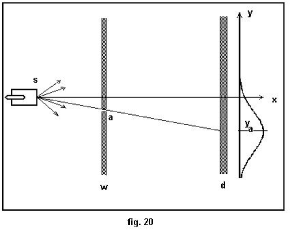
3 Double-Slit Experiment
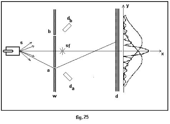
In vacuum (Fig. 1 2 3 s 𝑠 s w 𝑤 w d 𝑑 d [7 ] .
Electrons are emitted one by one from the source s 𝑠 s d 𝑑 d d 𝑑 d
1. Let slit a 𝑎 a w 𝑤 w 1 s 𝑠 s a 𝑎 a d 𝑑 d
If such operation will be reiterated N 𝑁 N N 𝑁 N d 𝑑 d a 𝑎 a y a subscript 𝑦 𝑎 y_{a}
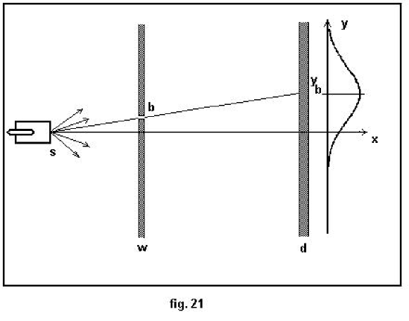
2. Let slit b 𝑏 b w 𝑤 w 2 s 𝑠 s b 𝑏 b d 𝑑 d
If such operation will be reiterated N 𝑁 N N 𝑁 N d 𝑑 d b 𝑏 b y b subscript 𝑦 𝑏 y_{b}
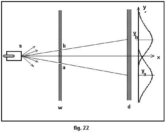
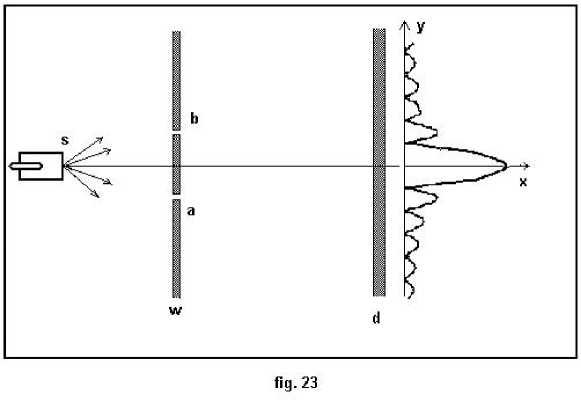
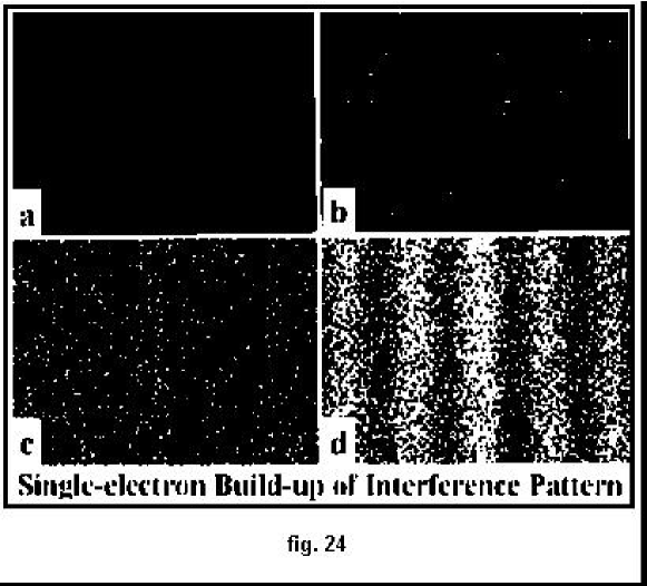
In this case the result like on fig. 3 is expected, isn’t it? But no. We get the same result as on
3. Let both slits be opened. In this case the result like Fig. 3 4 [8 ] .
For instance, such experiment was realized at Hitachi by A. Tonomura, J. Endo,
T. Matsuda, T. Kawasaki and H. Ezawa in 1989. It was presumed that interference fringes
are produced only when two electrons pass through both slits simultaneously. If there
were two electrons from the source s 𝑠 s 5 5 s 𝑠 s
4. But nevertheless, across which slit the electron has slipped?
Let (Fig. 6 d a subscript 𝑑 𝑎 d_{a} d b subscript 𝑑 𝑏 d_{b} s f 𝑠 𝑓 sf 4
An electron slipped across slit a 𝑎 a s f 𝑠 𝑓 sf d a subscript 𝑑 𝑎 d_{a} b 𝑏 b s f 𝑠 𝑓 sf d b subscript 𝑑 𝑏 d_{b}
If photon source s f 𝑠 𝑓 sf N 𝑁 N 3
If source s f 𝑠 𝑓 sf N 𝑁 N d a subscript 𝑑 𝑎 d_{a} d b subscript 𝑑 𝑏 d_{b} d a subscript 𝑑 𝑎 d_{a} d b subscript 𝑑 𝑏 d_{b} 3 4 6
Figure 1: Figure 2: Figure 3: Figure 4: Figure 5: Figure 6:
4 Event-Probability Interpretation
Let us try to interpret these experiments by events and probabilities.
Let source s 𝑠 s ⟨ x 0 , y 0 ⟩ subscript 𝑥 0 subscript 𝑦 0
\left\langle x_{0},y_{0}\right\rangle a 𝑎 a ⟨ x a , y a ⟩ subscript 𝑥 𝑎 subscript 𝑦 𝑎
\left\langle x_{a},y_{a}\right\rangle b 𝑏 b ⟨ x b , y b ⟩ subscript 𝑥 𝑏 subscript 𝑦 𝑏
\left\langle x_{b},y_{b}\right\rangle x a = x b subscript 𝑥 𝑎 subscript 𝑥 𝑏 x_{a}=x_{b} w 𝑤 w x = x a 𝑥 subscript 𝑥 𝑎 x=x_{a} d 𝑑 d x = x d 𝑥 subscript 𝑥 𝑑 x=x_{d}
Denote:
≪ much-less-than \ll ⟨ t , x , y ⟩ 𝑡 𝑥 𝑦
\left\langle t,x,y\right\rangle ≫ much-greater-than \gg 𝒞 ( t , x , y ) 𝒞 𝑡 𝑥 𝑦 \mathcal{C}\left(t,x,y\right) ≪ much-less-than \ll a 𝑎 a ≫ much-greater-than \gg 𝒜 𝒜 \mathcal{A} ≪ much-less-than \ll b 𝑏 b ≫ much-greater-than \gg ℬ ℬ \mathcal{B}
Let t 0 subscript 𝑡 0 t_{0} s 𝑠 s s 𝑠 s φ 𝒞 subscript 𝜑 𝒞 \varphi_{\mathcal{C}} t 0 subscript 𝑡 0 t_{0}
φ 𝒞 ( t , x , y ) | t = t 0 = φ 𝒞 ( t 0 , x , y ) δ ( x − x 0 ) δ ( y − y 0 ) . evaluated-at subscript 𝜑 𝒞 𝑡 𝑥 𝑦 𝑡 subscript 𝑡 0 subscript 𝜑 𝒞 subscript 𝑡 0 𝑥 𝑦 𝛿 𝑥 subscript 𝑥 0 𝛿 𝑦 subscript 𝑦 0 . \varphi_{\mathcal{C}}\left(t,x,y\right)|_{t=t_{0}}=\varphi_{\mathcal{C}}\left(t_{0},x,y\right)\delta\left(x-x_{0}\right)\delta\left(y-y_{0}\right)\mbox{.} (12)
Let t w subscript 𝑡 𝑤 t_{w} 𝒞 ( t , x , y ) 𝒞 𝑡 𝑥 𝑦 \mathcal{C}\left(t,x,y\right) 𝒞 ( t , x , y ) 𝒞 𝑡 𝑥 𝑦 \mathcal{C}\left(t,x,y\right) w 𝑤 w
Let t d subscript 𝑡 𝑑 t_{d} d 𝑑 d
1. Let slit a 𝑎 a w 𝑤 w 1
In that case the 𝒞 ( t , x , y ) 𝒞 𝑡 𝑥 𝑦 \mathcal{C}\left(t,x,y\right)
K 𝒞 𝒜 ( t − t 0 , x − x s , y − y s ) subscript 𝐾 𝒞 𝒜 𝑡 subscript 𝑡 0 𝑥 subscript 𝑥 𝑠 𝑦 subscript 𝑦 𝑠 K_{\mathcal{CA}}\left(t-t_{0},x-x_{s},y-y_{s}\right)
in instant t w subscript 𝑡 𝑤 t_{w}
K 𝒞 𝒜 ( t − t 0 , x − x s , y − y s ) | t = t w evaluated-at subscript 𝐾 𝒞 𝒜 𝑡 subscript 𝑡 0 𝑥 subscript 𝑥 𝑠 𝑦 subscript 𝑦 𝑠 𝑡 subscript 𝑡 𝑤 \displaystyle K_{\mathcal{CA}}\left(t-t_{0},x-x_{s},y-y_{s}\right)|_{t=t_{w}}
= \displaystyle= K 𝒞 𝒜 ( t w − t 0 , x − x s , y − y s ) δ ( x − x a ) δ ( y − y a ) . subscript 𝐾 𝒞 𝒜 subscript 𝑡 𝑤 subscript 𝑡 0 𝑥 subscript 𝑥 𝑠 𝑦 subscript 𝑦 𝑠 𝛿 𝑥 subscript 𝑥 𝑎 𝛿 𝑦 subscript 𝑦 𝑎 . \displaystyle K_{\mathcal{CA}}\left(t_{w}-t_{0},x-x_{s},y-y_{s}\right)\delta\left(x-x_{a}\right)\delta\left(y-y_{a}\right)\mbox{.}
According to the propagator property:
K ( t − t 0 , x − x s , y − y s ) = 𝐾 𝑡 subscript 𝑡 0 𝑥 subscript 𝑥 𝑠 𝑦 subscript 𝑦 𝑠 absent \displaystyle K\left(t-t_{0},x-x_{s},y-y_{s}\right)=
= \displaystyle= ∫ − π c h π c h d x 1 ∫ − π c h π c h d y 1 ⋅ K ( t − t 1 , x − x 1 , y − y 1 ) × \displaystyle\int_{-\frac{\pi\mathrm{c}}{\mathrm{h}}}^{\frac{\pi\mathrm{c}}{\mathrm{h}}}dx_{1}\int_{-\frac{\pi\mathrm{c}}{\mathrm{h}}}^{\frac{\pi\mathrm{c}}{\mathrm{h}}}dy_{1}\cdot K\left(t-t_{1},x-x_{1},y-y_{1}\right)\times
× K ( t 1 − t 0 , x 1 − x s , y 1 − y s ) . absent 𝐾 subscript 𝑡 1 subscript 𝑡 0 subscript 𝑥 1 subscript 𝑥 𝑠 subscript 𝑦 1 subscript 𝑦 𝑠 . \displaystyle\times K\left(t_{1}-t_{0},x_{1}-x_{s},y_{1}-y_{s}\right)\mbox{.}
K 𝒞 𝒜 ( t d − t 0 , x d − x s , y d − y s ) = subscript 𝐾 𝒞 𝒜 subscript 𝑡 𝑑 subscript 𝑡 0 subscript 𝑥 𝑑 subscript 𝑥 𝑠 subscript 𝑦 𝑑 subscript 𝑦 𝑠 absent \displaystyle K_{\mathcal{CA}}\left(t_{d}-t_{0},x_{d}-x_{s},y_{d}-y_{s}\right)=
= \displaystyle= ∫ − π c h π c h d x ∫ − π c h π c h d y ⋅ K 𝒞 𝒜 ( t d − t w , x d − x , y d − y ) × \displaystyle\int_{-\frac{\pi\mathrm{c}}{\mathrm{h}}}^{\frac{\pi\mathrm{c}}{\mathrm{h}}}dx\int_{-\frac{\pi\mathrm{c}}{\mathrm{h}}}^{\frac{\pi\mathrm{c}}{\mathrm{h}}}dy\cdot K_{\mathcal{CA}}\left(t_{d}-t_{w},x_{d}-x,y_{d}-y\right)\times
× K 𝒞 𝒜 ( t w − t 0 , x − x s , y − y s ) δ ( x − x a ) δ ( y − y a ) . absent subscript 𝐾 𝒞 𝒜 subscript 𝑡 𝑤 subscript 𝑡 0 𝑥 subscript 𝑥 𝑠 𝑦 subscript 𝑦 𝑠 𝛿 𝑥 subscript 𝑥 𝑎 𝛿 𝑦 subscript 𝑦 𝑎 . \displaystyle\times K_{\mathcal{CA}}\left(t_{w}-t_{0},x-x_{s},y-y_{s}\right)\delta\left(x-x_{a}\right)\delta\left(y-y_{a}\right)\mbox{.}
Therefore, according to properties of δ 𝛿 \delta
K 𝒞 𝒜 ( t d − t 0 , x d − x s , y d − y s ) = subscript 𝐾 𝒞 𝒜 subscript 𝑡 𝑑 subscript 𝑡 0 subscript 𝑥 𝑑 subscript 𝑥 𝑠 subscript 𝑦 𝑑 subscript 𝑦 𝑠 absent \displaystyle K_{\mathcal{CA}}\left(t_{d}-t_{0},x_{d}-x_{s},y_{d}-y_{s}\right)=
= \displaystyle= K 𝒞 𝒜 ( t d − t w , x d − x a , y d − y a ) K 𝒞 𝒜 ( t w − t 0 , x a − x s , y a − y s ) . subscript 𝐾 𝒞 𝒜 subscript 𝑡 𝑑 subscript 𝑡 𝑤 subscript 𝑥 𝑑 subscript 𝑥 𝑎 subscript 𝑦 𝑑 subscript 𝑦 𝑎 subscript 𝐾 𝒞 𝒜 subscript 𝑡 𝑤 subscript 𝑡 0 subscript 𝑥 𝑎 subscript 𝑥 𝑠 subscript 𝑦 𝑎 subscript 𝑦 𝑠 . \displaystyle K_{\mathcal{CA}}\left(t_{d}-t_{w},x_{d}-x_{a},y_{d}-y_{a}\right)K_{\mathcal{CA}}\left(t_{w}-t_{0},x_{a}-x_{s},y_{a}-y_{s}\right)\mbox{.}
The state vector for the event 𝒞 ( t , x , y ) 𝒞 𝑡 𝑥 𝑦 \mathcal{C}\left(t,x,y\right) 𝒜 𝒜 \mathcal{A} 11
φ 𝒞 𝒜 ( t d , x d , y d ) = subscript 𝜑 𝒞 𝒜 subscript 𝑡 𝑑 subscript 𝑥 𝑑 subscript 𝑦 𝑑 absent \displaystyle\varphi_{\mathcal{CA}}\left(t_{d},x_{d},y_{d}\right)=
= \displaystyle= ∫ − π c h π c h 𝑑 x s ∫ − π c h π c h 𝑑 y s ⋅ K 𝒞 𝒜 ( t d − t 0 , x d − x s , y d − y s ) φ 𝒞 ( t 0 , x s , y s ) . superscript subscript 𝜋 c h 𝜋 c h differential-d subscript 𝑥 𝑠 superscript subscript 𝜋 c h 𝜋 c h ⋅ differential-d subscript 𝑦 𝑠 subscript 𝐾 𝒞 𝒜 subscript 𝑡 𝑑 subscript 𝑡 0 subscript 𝑥 𝑑 subscript 𝑥 𝑠 subscript 𝑦 𝑑 subscript 𝑦 𝑠 subscript 𝜑 𝒞 subscript 𝑡 0 subscript 𝑥 𝑠 subscript 𝑦 𝑠 . \displaystyle\int_{-\frac{\pi\mathrm{c}}{\mathrm{h}}}^{\frac{\pi\mathrm{c}}{\mathrm{h}}}dx_{s}\int_{-\frac{\pi\mathrm{c}}{\mathrm{h}}}^{\frac{\pi\mathrm{c}}{\mathrm{h}}}dy_{s}\cdot K_{\mathcal{CA}}\left(t_{d}-t_{0},x_{d}-x_{s},y_{d}-y_{s}\right)\varphi_{\mathcal{C}}\left(t_{0},x_{s},y_{s}\right)\mbox{.}
φ 𝒞 𝒜 ( t d , x d , y d ) subscript 𝜑 𝒞 𝒜 subscript 𝑡 𝑑 subscript 𝑥 𝑑 subscript 𝑦 𝑑 \displaystyle\varphi_{\mathcal{CA}}\left(t_{d},x_{d},y_{d}\right) = \displaystyle= ∫ − π c h π c h 𝑑 x s ∫ − π c h π c h 𝑑 y s ⋅ K 𝒞 𝒜 ( t d − t 0 , x d − x s , y d − y s ) superscript subscript 𝜋 c h 𝜋 c h differential-d subscript 𝑥 𝑠 superscript subscript 𝜋 c h 𝜋 c h ⋅ differential-d subscript 𝑦 𝑠 subscript 𝐾 𝒞 𝒜 subscript 𝑡 𝑑 subscript 𝑡 0 subscript 𝑥 𝑑 subscript 𝑥 𝑠 subscript 𝑦 𝑑 subscript 𝑦 𝑠 \displaystyle\int_{-\frac{\pi\mathrm{c}}{\mathrm{h}}}^{\frac{\pi\mathrm{c}}{\mathrm{h}}}dx_{s}\int_{-\frac{\pi\mathrm{c}}{\mathrm{h}}}^{\frac{\pi\mathrm{c}}{\mathrm{h}}}dy_{s}\cdot K_{\mathcal{CA}}\left(t_{d}-t_{0},x_{d}-x_{s},y_{d}-y_{s}\right)
φ 𝒞 ( t 0 , x s , y s ) δ ( x s − x 0 ) δ ( y s − y 0 ) . subscript 𝜑 𝒞 subscript 𝑡 0 subscript 𝑥 𝑠 subscript 𝑦 𝑠 𝛿 subscript 𝑥 𝑠 subscript 𝑥 0 𝛿 subscript 𝑦 𝑠 subscript 𝑦 0 . \displaystyle\varphi_{\mathcal{C}}\left(t_{0},x_{s},y_{s}\right)\delta\left(x_{s}-x_{0}\right)\delta\left(y_{s}-y_{0}\right)\mbox{.}
φ 𝒞 𝒜 ( t d , x d , y d ) = subscript 𝜑 𝒞 𝒜 subscript 𝑡 𝑑 subscript 𝑥 𝑑 subscript 𝑦 𝑑 absent \displaystyle\varphi_{\mathcal{CA}}\left(t_{d},x_{d},y_{d}\right)=
= ∫ − π c h π c h 𝑑 x s ∫ − π c h π c h 𝑑 y s ⋅ K 𝒞 𝒜 ( t d − t w , x d − x a , y d − y a ) absent superscript subscript 𝜋 c h 𝜋 c h differential-d subscript 𝑥 𝑠 superscript subscript 𝜋 c h 𝜋 c h ⋅ differential-d subscript 𝑦 𝑠 subscript 𝐾 𝒞 𝒜 subscript 𝑡 𝑑 subscript 𝑡 𝑤 subscript 𝑥 𝑑 subscript 𝑥 𝑎 subscript 𝑦 𝑑 subscript 𝑦 𝑎 \displaystyle=\int\limits_{-\frac{\pi\mathrm{c}}{\mathrm{h}}}^{\frac{\pi\mathrm{c}}{\mathrm{h}}}dx_{s}\int\limits_{-\frac{\pi\mathrm{c}}{\mathrm{h}}}^{\frac{\pi\mathrm{c}}{\mathrm{h}}}dy_{s}\cdot K_{\mathcal{CA}}\left(t_{d}-t_{w},x_{d}-x_{a},y_{d}-y_{a}\right)
× K 𝒞 𝒜 ( t w − t 0 , x a − x s , y a − y s ) × \displaystyle\times K_{\mathcal{CA}}\left(t_{w}-t_{0},x_{a}-x_{s},y_{a}-y_{s}\right)\times
× φ 𝒞 ( t 0 , x s , y s ) δ ( x s − x 0 ) δ ( y s − y 0 ) . absent subscript 𝜑 𝒞 subscript 𝑡 0 subscript 𝑥 𝑠 subscript 𝑦 𝑠 𝛿 subscript 𝑥 𝑠 subscript 𝑥 0 𝛿 subscript 𝑦 𝑠 subscript 𝑦 0 . \displaystyle\times\varphi_{\mathcal{C}}\left(t_{0},x_{s},y_{s}\right)\delta\left(x_{s}-x_{0}\right)\delta\left(y_{s}-y_{0}\right)\mbox{.}
Hence, according to properties of δ 𝛿 \delta
φ 𝒞 𝒜 ( t d , x d , y d ) = subscript 𝜑 𝒞 𝒜 subscript 𝑡 𝑑 subscript 𝑥 𝑑 subscript 𝑦 𝑑 absent \displaystyle\varphi_{\mathcal{CA}}\left(t_{d},x_{d},y_{d}\right)=
= K 𝒞 𝒜 ( t d − t w , x d − x a , y d − y a ) absent subscript 𝐾 𝒞 𝒜 subscript 𝑡 𝑑 subscript 𝑡 𝑤 subscript 𝑥 𝑑 subscript 𝑥 𝑎 subscript 𝑦 𝑑 subscript 𝑦 𝑎 \displaystyle=K_{\mathcal{CA}}\left(t_{d}-t_{w},x_{d}-x_{a},y_{d}-y_{a}\right)
K 𝒞 𝒜 ( t w − t 0 , x a − x 0 , y a − y 0 ) subscript 𝐾 𝒞 𝒜 subscript 𝑡 𝑤 subscript 𝑡 0 subscript 𝑥 𝑎 subscript 𝑥 0 subscript 𝑦 𝑎 subscript 𝑦 0 \displaystyle K_{\mathcal{CA}}\left(t_{w}-t_{0},x_{a}-x_{0},y_{a}-y_{0}\right)
φ 𝒞 ( t 0 , x 0 , y 0 ) . subscript 𝜑 𝒞 subscript 𝑡 0 subscript 𝑥 0 subscript 𝑦 0 . \displaystyle\varphi_{\mathcal{C}}\left(t_{0},x_{0},y_{0}\right)\mbox{.}
ρ 𝒞 𝒜 ( t d , x d , y d ) = φ 𝒞 𝒜 † ( t d , x d , y d ) φ 𝒞 𝒜 ( t d , x d , y d ) . subscript 𝜌 𝒞 𝒜 subscript 𝑡 𝑑 subscript 𝑥 𝑑 subscript 𝑦 𝑑 superscript subscript 𝜑 𝒞 𝒜 † subscript 𝑡 𝑑 subscript 𝑥 𝑑 subscript 𝑦 𝑑 subscript 𝜑 𝒞 𝒜 subscript 𝑡 𝑑 subscript 𝑥 𝑑 subscript 𝑦 𝑑 . \rho_{\mathcal{CA}}\left(t_{d},x_{d},y_{d}\right)=\varphi_{\mathcal{CA}}^{\dagger}\left(t_{d},x_{d},y_{d}\right)\varphi_{\mathcal{CA}}\left(t_{d},x_{d},y_{d}\right)\mbox{.}
Therefore, a probability to detect the electron in vicinity Δ x Δ y Δ 𝑥 Δ 𝑦 \Delta x\Delta y ⟨ x d , y d ⟩ subscript 𝑥 𝑑 subscript 𝑦 𝑑
\left\langle x_{d},y_{d}\right\rangle t 𝑡 t 𝒜 𝒜 \mathcal{A}
P a ( t d , x d , y d ) := P ( 𝒞 ( t d , Δ x Δ y ) / 𝒜 ) = ρ 𝒞 𝒜 ( t d , x d , y d ) Δ x Δ y . assign subscript 𝑃 𝑎 subscript 𝑡 𝑑 subscript 𝑥 𝑑 subscript 𝑦 𝑑 P 𝒞 subscript 𝑡 𝑑 Δ 𝑥 Δ 𝑦 𝒜 subscript 𝜌 𝒞 𝒜 subscript 𝑡 𝑑 subscript 𝑥 𝑑 subscript 𝑦 𝑑 Δ 𝑥 Δ 𝑦 . P_{a}\left(t_{d},x_{d},y_{d}\right):=\mathrm{P}\left(\mathcal{C}\left(t_{d},\Delta x\Delta y\right)/\mathcal{A}\right)=\rho_{\mathcal{CA}}\left(t_{d},x_{d},y_{d}\right)\Delta x\Delta y\mbox{.}
2. Let slit b 𝑏 b w 𝑤 w 2
In that case the 𝒞 ( t , x , y ) 𝒞 𝑡 𝑥 𝑦 \mathcal{C}\left(t,x,y\right)
K 𝒞 ℬ ( t − t 0 , x − x s , y − y s ) subscript 𝐾 𝒞 ℬ 𝑡 subscript 𝑡 0 𝑥 subscript 𝑥 𝑠 𝑦 subscript 𝑦 𝑠 K_{\mathcal{CB}}\left(t-t_{0},x-x_{s},y-y_{s}\right)
in instant t w subscript 𝑡 𝑤 t_{w}
K 𝒞 ℬ ( t − t 0 , x − x s , y − y s ) | t = t w evaluated-at subscript 𝐾 𝒞 ℬ 𝑡 subscript 𝑡 0 𝑥 subscript 𝑥 𝑠 𝑦 subscript 𝑦 𝑠 𝑡 subscript 𝑡 𝑤 \displaystyle K_{\mathcal{CB}}\left(t-t_{0},x-x_{s},y-y_{s}\right)|_{t=t_{w}}
= \displaystyle= K 𝒞 ℬ ( t w − t 0 , x − x s , y − y s ) δ ( x − x b ) δ ( y − y b ) . subscript 𝐾 𝒞 ℬ subscript 𝑡 𝑤 subscript 𝑡 0 𝑥 subscript 𝑥 𝑠 𝑦 subscript 𝑦 𝑠 𝛿 𝑥 subscript 𝑥 𝑏 𝛿 𝑦 subscript 𝑦 𝑏 . \displaystyle K_{\mathcal{CB}}\left(t_{w}-t_{0},x-x_{s},y-y_{s}\right)\delta\left(x-x_{b}\right)\delta\left(y-y_{b}\right)\mbox{.}
Hence, according to the propagator property:
K 𝒞 ℬ ( t d − t 0 , x d − x s , y d − y s ) = subscript 𝐾 𝒞 ℬ subscript 𝑡 𝑑 subscript 𝑡 0 subscript 𝑥 𝑑 subscript 𝑥 𝑠 subscript 𝑦 𝑑 subscript 𝑦 𝑠 absent \displaystyle K_{\mathcal{CB}}\left(t_{d}-t_{0},x_{d}-x_{s},y_{d}-y_{s}\right)=
= \displaystyle= ∫ − π c h π c h 𝑑 x ∫ − π c h π c h 𝑑 y ⋅ K 𝒞 ℬ ( t d − t w , x d − x , y d − y ) superscript subscript 𝜋 c h 𝜋 c h differential-d 𝑥 superscript subscript 𝜋 c h 𝜋 c h ⋅ differential-d 𝑦 subscript 𝐾 𝒞 ℬ subscript 𝑡 𝑑 subscript 𝑡 𝑤 subscript 𝑥 𝑑 𝑥 subscript 𝑦 𝑑 𝑦 \displaystyle\int\limits_{-\frac{\pi\mathrm{c}}{\mathrm{h}}}^{\frac{\pi\mathrm{c}}{\mathrm{h}}}dx\int\limits_{-\frac{\pi\mathrm{c}}{\mathrm{h}}}^{\frac{\pi\mathrm{c}}{\mathrm{h}}}dy\cdot K_{\mathcal{CB}}\left(t_{d}-t_{w},x_{d}-x,y_{d}-y\right)
K 𝒞 ℬ ( t w − t 0 , x − x s , y − y s ) δ ( x − x b ) δ ( y − y b ) . subscript 𝐾 𝒞 ℬ subscript 𝑡 𝑤 subscript 𝑡 0 𝑥 subscript 𝑥 𝑠 𝑦 subscript 𝑦 𝑠 𝛿 𝑥 subscript 𝑥 𝑏 𝛿 𝑦 subscript 𝑦 𝑏 . \displaystyle K_{\mathcal{CB}}\left(t_{w}-t_{0},x-x_{s},y-y_{s}\right)\delta\left(x-x_{b}\right)\delta\left(y-y_{b}\right)\mbox{.}
Therefore, according to properties of δ 𝛿 \delta
K 𝒞 ℬ ( t d − t 0 , x d − x s , y d − y s ) = subscript 𝐾 𝒞 ℬ subscript 𝑡 𝑑 subscript 𝑡 0 subscript 𝑥 𝑑 subscript 𝑥 𝑠 subscript 𝑦 𝑑 subscript 𝑦 𝑠 absent \displaystyle K_{\mathcal{CB}}\left(t_{d}-t_{0},x_{d}-x_{s},y_{d}-y_{s}\right)=
= \displaystyle= K 𝒞 ℬ ( t d − t w , x d − x b , y d − y b ) K 𝒞 ℬ ( t w − t 0 , x b − x s , y b − y s ) . subscript 𝐾 𝒞 ℬ subscript 𝑡 𝑑 subscript 𝑡 𝑤 subscript 𝑥 𝑑 subscript 𝑥 𝑏 subscript 𝑦 𝑑 subscript 𝑦 𝑏 subscript 𝐾 𝒞 ℬ subscript 𝑡 𝑤 subscript 𝑡 0 subscript 𝑥 𝑏 subscript 𝑥 𝑠 subscript 𝑦 𝑏 subscript 𝑦 𝑠 . \displaystyle K_{\mathcal{CB}}\left(t_{d}-t_{w},x_{d}-x_{b},y_{d}-y_{b}\right)K_{\mathcal{CB}}\left(t_{w}-t_{0},x_{b}-x_{s},y_{b}-y_{s}\right)\mbox{.}
The state vector for the event 𝒞 ( t , x , y ) 𝒞 𝑡 𝑥 𝑦 \mathcal{C}\left(t,x,y\right) ℬ ℬ \mathcal{B} 11
φ 𝒞 ℬ ( t d , x d , y d ) = subscript 𝜑 𝒞 ℬ subscript 𝑡 𝑑 subscript 𝑥 𝑑 subscript 𝑦 𝑑 absent \displaystyle\varphi_{\mathcal{CB}}\left(t_{d},x_{d},y_{d}\right)=
= \displaystyle= ∫ − π c h π c h 𝑑 x s ∫ − π c h π c h 𝑑 y s ⋅ K 𝒞 ℬ ( t d − t 0 , x d − x s , y d − y s ) φ 𝒞 ( t 0 , x s , y s ) . superscript subscript 𝜋 c h 𝜋 c h differential-d subscript 𝑥 𝑠 superscript subscript 𝜋 c h 𝜋 c h ⋅ differential-d subscript 𝑦 𝑠 subscript 𝐾 𝒞 ℬ subscript 𝑡 𝑑 subscript 𝑡 0 subscript 𝑥 𝑑 subscript 𝑥 𝑠 subscript 𝑦 𝑑 subscript 𝑦 𝑠 subscript 𝜑 𝒞 subscript 𝑡 0 subscript 𝑥 𝑠 subscript 𝑦 𝑠 . \displaystyle\int_{-\frac{\pi\mathrm{c}}{\mathrm{h}}}^{\frac{\pi\mathrm{c}}{\mathrm{h}}}dx_{s}\int_{-\frac{\pi\mathrm{c}}{\mathrm{h}}}^{\frac{\pi\mathrm{c}}{\mathrm{h}}}dy_{s}\cdot K_{\mathcal{CB}}\left(t_{d}-t_{0},x_{d}-x_{s},y_{d}-y_{s}\right)\varphi_{\mathcal{C}}\left(t_{0},x_{s},y_{s}\right)\mbox{.}
φ 𝒞 ℬ ( t d , x d , y d ) subscript 𝜑 𝒞 ℬ subscript 𝑡 𝑑 subscript 𝑥 𝑑 subscript 𝑦 𝑑 \displaystyle\varphi_{\mathcal{CB}}\left(t_{d},x_{d},y_{d}\right) = \displaystyle= ∫ − π c h π c h 𝑑 x s ∫ − π c h π c h 𝑑 y s ⋅ K 𝒞 ℬ ( t d − t 0 , x d − x s , y d − y s ) superscript subscript 𝜋 c h 𝜋 c h differential-d subscript 𝑥 𝑠 superscript subscript 𝜋 c h 𝜋 c h ⋅ differential-d subscript 𝑦 𝑠 subscript 𝐾 𝒞 ℬ subscript 𝑡 𝑑 subscript 𝑡 0 subscript 𝑥 𝑑 subscript 𝑥 𝑠 subscript 𝑦 𝑑 subscript 𝑦 𝑠 \displaystyle\int_{-\frac{\pi\mathrm{c}}{\mathrm{h}}}^{\frac{\pi\mathrm{c}}{\mathrm{h}}}dx_{s}\int_{-\frac{\pi\mathrm{c}}{\mathrm{h}}}^{\frac{\pi\mathrm{c}}{\mathrm{h}}}dy_{s}\cdot K_{\mathcal{CB}}\left(t_{d}-t_{0},x_{d}-x_{s},y_{d}-y_{s}\right)
× φ 𝒞 ( t 0 , x s , y s ) δ ( x s − x 0 ) δ ( y s − y 0 ) . absent subscript 𝜑 𝒞 subscript 𝑡 0 subscript 𝑥 𝑠 subscript 𝑦 𝑠 𝛿 subscript 𝑥 𝑠 subscript 𝑥 0 𝛿 subscript 𝑦 𝑠 subscript 𝑦 0 . \displaystyle\times\varphi_{\mathcal{C}}\left(t_{0},x_{s},y_{s}\right)\delta\left(x_{s}-x_{0}\right)\delta\left(y_{s}-y_{0}\right)\mbox{.}
φ 𝒞 ℬ ( t d , x d , y d ) = subscript 𝜑 𝒞 ℬ subscript 𝑡 𝑑 subscript 𝑥 𝑑 subscript 𝑦 𝑑 absent \displaystyle\varphi_{\mathcal{CB}}\left(t_{d},x_{d},y_{d}\right)=
= ∫ − π c h π c h 𝑑 x s ∫ − π c h π c h 𝑑 y s ⋅ K 𝒞 ℬ ( t d − t w , x d − x b , y d − y b ) absent superscript subscript 𝜋 c h 𝜋 c h differential-d subscript 𝑥 𝑠 superscript subscript 𝜋 c h 𝜋 c h ⋅ differential-d subscript 𝑦 𝑠 subscript 𝐾 𝒞 ℬ subscript 𝑡 𝑑 subscript 𝑡 𝑤 subscript 𝑥 𝑑 subscript 𝑥 𝑏 subscript 𝑦 𝑑 subscript 𝑦 𝑏 \displaystyle=\int\limits_{-\frac{\pi\mathrm{c}}{\mathrm{h}}}^{\frac{\pi\mathrm{c}}{\mathrm{h}}}dx_{s}\int\limits_{-\frac{\pi\mathrm{c}}{\mathrm{h}}}^{\frac{\pi\mathrm{c}}{\mathrm{h}}}dy_{s}\cdot K_{\mathcal{CB}}\left(t_{d}-t_{w},x_{d}-x_{b},y_{d}-y_{b}\right)
× K 𝒞 ℬ ( t w − t 0 , x b − x s , y b − y s ) absent subscript 𝐾 𝒞 ℬ subscript 𝑡 𝑤 subscript 𝑡 0 subscript 𝑥 𝑏 subscript 𝑥 𝑠 subscript 𝑦 𝑏 subscript 𝑦 𝑠 \displaystyle\times K_{\mathcal{CB}}\left(t_{w}-t_{0},x_{b}-x_{s},y_{b}-y_{s}\right)
× φ 𝒞 ( t 0 , x s , y s ) δ ( x s − x 0 ) δ ( y s − y 0 ) . absent subscript 𝜑 𝒞 subscript 𝑡 0 subscript 𝑥 𝑠 subscript 𝑦 𝑠 𝛿 subscript 𝑥 𝑠 subscript 𝑥 0 𝛿 subscript 𝑦 𝑠 subscript 𝑦 0 . \displaystyle\times\varphi_{\mathcal{C}}\left(t_{0},x_{s},y_{s}\right)\delta\left(x_{s}-x_{0}\right)\delta\left(y_{s}-y_{0}\right)\mbox{.}
Hence, according to properties of δ 𝛿 \delta
φ 𝒞 ℬ ( t d , x d , y d ) = subscript 𝜑 𝒞 ℬ subscript 𝑡 𝑑 subscript 𝑥 𝑑 subscript 𝑦 𝑑 absent \displaystyle\varphi_{\mathcal{CB}}\left(t_{d},x_{d},y_{d}\right)=
= K 𝒞 ℬ ( t d − t w , x d − x b , y d − y b ) × \displaystyle=K_{\mathcal{CB}}\left(t_{d}-t_{w},x_{d}-x_{b},y_{d}-y_{b}\right)\times
K 𝒞 ℬ ( t w − t 0 , x b − x 0 , y b − y 0 ) × \displaystyle K_{\mathcal{CB}}\left(t_{w}-t_{0},x_{b}-x_{0},y_{b}-y_{0}\right)\times
φ 𝒞 ( t 0 , x 0 , y 0 ) . subscript 𝜑 𝒞 subscript 𝑡 0 subscript 𝑥 0 subscript 𝑦 0 . \displaystyle\varphi_{\mathcal{C}}\left(t_{0},x_{0},y_{0}\right)\mbox{.}
ρ 𝒞 ℬ ( t d , x d , y d ) = φ 𝒞 ℬ † ( t d , x d , y d ) φ 𝒞 ℬ ( t d , x d , y d ) . subscript 𝜌 𝒞 ℬ subscript 𝑡 𝑑 subscript 𝑥 𝑑 subscript 𝑦 𝑑 superscript subscript 𝜑 𝒞 ℬ † subscript 𝑡 𝑑 subscript 𝑥 𝑑 subscript 𝑦 𝑑 subscript 𝜑 𝒞 ℬ subscript 𝑡 𝑑 subscript 𝑥 𝑑 subscript 𝑦 𝑑 . \rho_{\mathcal{CB}}\left(t_{d},x_{d},y_{d}\right)=\varphi_{\mathcal{CB}}^{\dagger}\left(t_{d},x_{d},y_{d}\right)\varphi_{\mathcal{CB}}\left(t_{d},x_{d},y_{d}\right)\mbox{.}
Therefore, a probability to detect the electron in vicinity Δ x Δ y Δ 𝑥 Δ 𝑦 \Delta x\Delta y ⟨ x d , y d ⟩ subscript 𝑥 𝑑 subscript 𝑦 𝑑
\left\langle x_{d},y_{d}\right\rangle t 𝑡 t ℬ ℬ \mathcal{B}
P b ( t d , x d , y d ) := P ( 𝒞 ( t d , Δ x Δ y ) / ℬ ) = ρ 𝒞 ℬ ( t d , x d , y d ) Δ x Δ y . assign subscript 𝑃 𝑏 subscript 𝑡 𝑑 subscript 𝑥 𝑑 subscript 𝑦 𝑑 P 𝒞 subscript 𝑡 𝑑 Δ 𝑥 Δ 𝑦 ℬ subscript 𝜌 𝒞 ℬ subscript 𝑡 𝑑 subscript 𝑥 𝑑 subscript 𝑦 𝑑 Δ 𝑥 Δ 𝑦 . P_{b}\left(t_{d},x_{d},y_{d}\right):=\mathrm{P}\left(\mathcal{C}\left(t_{d},\Delta x\Delta y\right)/\mathcal{B}\right)=\rho_{\mathcal{CB}}\left(t_{d},x_{d},y_{d}\right)\Delta x\Delta y\mbox{.}
3. Let both slits and a 𝑎 a b 𝑏 b 4
In that case the 𝒞 ( t , x , y ) 𝒞 𝑡 𝑥 𝑦 \mathcal{C}\left(t,x,y\right)
K 𝒞 𝒜 ℬ ( t − t 0 , x − x s , y − y s ) subscript 𝐾 𝒞 𝒜 ℬ 𝑡 subscript 𝑡 0 𝑥 subscript 𝑥 𝑠 𝑦 subscript 𝑦 𝑠 K_{\mathcal{CAB}}\left(t-t_{0},x-x_{s},y-y_{s}\right)
in instant t w subscript 𝑡 𝑤 t_{w}
K 𝒞 𝒜 ℬ ( t − t 0 , x − x s , y − y s ) | t = t w = = K 𝒞 𝒜 ℬ ( t w − t 0 , x − x s , y − y s ) × ( δ ( x − x a ) δ ( y − y a ) + δ ( x − x b ) δ ( y − y b ) ) . \begin{array}[]{c}\ K_{\mathcal{CAB}}\left(t-t_{0},x-x_{s},y-y_{s}\right)|_{t=t_{w}}=\\
=K_{\mathcal{CAB}}\left(t_{w}-t_{0},x-x_{s},y-y_{s}\right)\times\\
\left(\delta\left(x-x_{a}\right)\delta\left(y-y_{a}\right)+\delta\left(x-x_{b}\right)\delta\left(y-y_{b}\right)\right)\mbox{.}\end{array}
Hence, according to the propagator property:
K 𝒞 𝒜 ℬ ( t d − t 0 , x d − x s , y d − y s ) = = ∫ − π c h π c h 𝑑 x ∫ − π c h π c h 𝑑 y ⋅ K 𝒞 𝒜 ℬ ( t d − t w , x d − x , y d − y ) × K 𝒞 𝒜 ℬ ( t w − t 0 , x − x s , y − y s ) × ( δ ( x − x a ) δ ( y − y a ) + δ ( x − x b ) δ ( y − y b ) ) . subscript 𝐾 𝒞 𝒜 ℬ subscript 𝑡 𝑑 subscript 𝑡 0 subscript 𝑥 𝑑 subscript 𝑥 𝑠 subscript 𝑦 𝑑 subscript 𝑦 𝑠 absent absent superscript subscript 𝜋 c h 𝜋 c h differential-d 𝑥 superscript subscript 𝜋 c h 𝜋 c h ⋅ differential-d 𝑦 subscript 𝐾 𝒞 𝒜 ℬ subscript 𝑡 𝑑 subscript 𝑡 𝑤 subscript 𝑥 𝑑 𝑥 subscript 𝑦 𝑑 𝑦 absent subscript 𝐾 𝒞 𝒜 ℬ subscript 𝑡 𝑤 subscript 𝑡 0 𝑥 subscript 𝑥 𝑠 𝑦 subscript 𝑦 𝑠 absent 𝛿 𝑥 subscript 𝑥 𝑎 𝛿 𝑦 subscript 𝑦 𝑎 𝛿 𝑥 subscript 𝑥 𝑏 𝛿 𝑦 subscript 𝑦 𝑏 . \begin{array}[]{c}\ K_{\mathcal{CAB}}\left(t_{d}-t_{0},x_{d}-x_{s},y_{d}-y_{s}\right)=\\
\ =\int\limits_{-\frac{\pi\mathrm{c}}{\mathrm{h}}}^{\frac{\pi\mathrm{c}}{\mathrm{h}}}dx\int\limits_{-\frac{\pi\mathrm{c}}{\mathrm{h}}}^{\frac{\pi\mathrm{c}}{\mathrm{h}}}dy\cdot K_{\mathcal{CAB}}\left(t_{d}-t_{w},x_{d}-x,y_{d}-y\right)\\
\times K_{\mathcal{CAB}}\left(t_{w}-t_{0},x-x_{s},y-y_{s}\right)\\
\times\left(\delta\left(x-x_{a}\right)\delta\left(y-y_{a}\right)+\delta\left(x-x_{b}\right)\delta\left(y-y_{b}\right)\right)\mbox{.}\end{array}
K 𝒞 𝒜 ℬ ( t d − t 0 , x d − x s , y d − y s ) = ∫ − π c h π c h 𝑑 x ∫ − π c h π c h 𝑑 y ⋅ K 𝒞 𝒜 ℬ ( t d − t w , x d − x , y d − y ) × K 𝒞 𝒜 ℬ ( t w − t 0 , x − x s , y − y s ) × × δ ( x − x a ) δ ( y − y a ) + ∫ − π c h π c h 𝑑 x ∫ − π c h π c h 𝑑 y ⋅ K 𝒞 𝒜 ℬ ( t d − t w , x d − x , y d − y ) × K 𝒞 𝒜 ℬ ( t w − t 0 , x − x s , y − y s ) × × δ ( x − x b ) δ ( y − y b ) . \begin{array}[]{c}\ K_{\mathcal{CAB}}\left(t_{d}-t_{0},x_{d}-x_{s},y_{d}-y_{s}\right)=\\
\begin{array}[]{c}\int\limits_{-\frac{\pi\mathrm{c}}{\mathrm{h}}}^{\frac{\pi\mathrm{c}}{\mathrm{h}}}dx\int\limits_{-\frac{\pi\mathrm{c}}{\mathrm{h}}}^{\frac{\pi\mathrm{c}}{\mathrm{h}}}dy\cdot K_{\mathcal{CAB}}\left(t_{d}-t_{w},x_{d}-x,y_{d}-y\right)\\
\times K_{\mathcal{CAB}}\left(t_{w}-t_{0},x-x_{s},y-y_{s}\right)\times\\
\times\delta\left(x-x_{a}\right)\delta\left(y-y_{a}\right)\\
+\int\limits_{-\frac{\pi\mathrm{c}}{\mathrm{h}}}^{\frac{\pi\mathrm{c}}{\mathrm{h}}}dx\int\limits_{-\frac{\pi\mathrm{c}}{\mathrm{h}}}^{\frac{\pi\mathrm{c}}{\mathrm{h}}}dy\cdot K_{\mathcal{CAB}}\left(t_{d}-t_{w},x_{d}-x,y_{d}-y\right)\\
\times K_{\mathcal{CAB}}\left(t_{w}-t_{0},x-x_{s},y-y_{s}\right)\times\\
\times\delta\left(x-x_{b}\right)\delta\left(y-y_{b}\right)\mbox{.}\end{array}\end{array}
Hence, according to properties of δ 𝛿 \delta
K 𝒞 𝒜 ℬ ( t d − t 0 , x d − x s , y d − y s ) = K 𝒞 𝒜 ℬ ( t d − t w , x d − x a , y d − y a ) K 𝒞 𝒜 ℬ ( t w − t 0 , x a − x s , y a − y s ) + K 𝒞 𝒜 ℬ ( t d − t w , x d − x b , y d − y b ) K 𝒞 𝒜 ℬ ( t w − t 0 , x b − x s , y b − y s ) . subscript 𝐾 𝒞 𝒜 ℬ subscript 𝑡 𝑑 subscript 𝑡 0 subscript 𝑥 𝑑 subscript 𝑥 𝑠 subscript 𝑦 𝑑 subscript 𝑦 𝑠 absent subscript 𝐾 𝒞 𝒜 ℬ subscript 𝑡 𝑑 subscript 𝑡 𝑤 subscript 𝑥 𝑑 subscript 𝑥 𝑎 subscript 𝑦 𝑑 subscript 𝑦 𝑎 subscript 𝐾 𝒞 𝒜 ℬ subscript 𝑡 𝑤 subscript 𝑡 0 subscript 𝑥 𝑎 subscript 𝑥 𝑠 subscript 𝑦 𝑎 subscript 𝑦 𝑠 subscript 𝐾 𝒞 𝒜 ℬ subscript 𝑡 𝑑 subscript 𝑡 𝑤 subscript 𝑥 𝑑 subscript 𝑥 𝑏 subscript 𝑦 𝑑 subscript 𝑦 𝑏 subscript 𝐾 𝒞 𝒜 ℬ subscript 𝑡 𝑤 subscript 𝑡 0 subscript 𝑥 𝑏 subscript 𝑥 𝑠 subscript 𝑦 𝑏 subscript 𝑦 𝑠 . \begin{array}[]{c}\ K_{\mathcal{CAB}}\left(t_{d}-t_{0},x_{d}-x_{s},y_{d}-y_{s}\right)=\\
\begin{array}[]{c}K_{\mathcal{CAB}}\left(t_{d}-t_{w},x_{d}-x_{a},y_{d}-y_{a}\right)\ K_{\mathcal{CAB}}\left(t_{w}-t_{0},x_{a}-x_{s},y_{a}-y_{s}\right)\\
+K_{\mathcal{CAB}}\left(t_{d}-t_{w},x_{d}-x_{b},y_{d}-y_{b}\right)\ K_{\mathcal{CAB}}\left(t_{w}-t_{0},x_{b}-x_{s},y_{b}-y_{s}\right)\end{array}\mbox{.}\end{array}
The state vector for the event 𝒞 ( t , x , y ) 𝒞 𝑡 𝑥 𝑦 \mathcal{C}\left(t,x,y\right) 𝒜 𝒜 \mathcal{A} ℬ ℬ \mathcal{B} 11
φ 𝒞 𝒜 ℬ ( t d , x d , y d ) = subscript 𝜑 𝒞 𝒜 ℬ subscript 𝑡 𝑑 subscript 𝑥 𝑑 subscript 𝑦 𝑑 absent \displaystyle\varphi_{\mathcal{CAB}}\left(t_{d},x_{d},y_{d}\right)=
= ∫ − π c h π c h 𝑑 x s ∫ − π c h π c h 𝑑 y s ⋅ K 𝒞 𝒜 ℬ ( t d − t 0 , x d − x s , y d − y s ) φ 𝒞 ( t 0 , x s , y s ) . absent superscript subscript 𝜋 c h 𝜋 c h differential-d subscript 𝑥 𝑠 superscript subscript 𝜋 c h 𝜋 c h ⋅ differential-d subscript 𝑦 𝑠 subscript 𝐾 𝒞 𝒜 ℬ subscript 𝑡 𝑑 subscript 𝑡 0 subscript 𝑥 𝑑 subscript 𝑥 𝑠 subscript 𝑦 𝑑 subscript 𝑦 𝑠 subscript 𝜑 𝒞 subscript 𝑡 0 subscript 𝑥 𝑠 subscript 𝑦 𝑠 . \displaystyle=\int\limits_{-\frac{\pi\mathrm{c}}{\mathrm{h}}}^{\frac{\pi\mathrm{c}}{\mathrm{h}}}dx_{s}\int\limits_{-\frac{\pi\mathrm{c}}{\mathrm{h}}}^{\frac{\pi\mathrm{c}}{\mathrm{h}}}dy_{s}\cdot K_{\mathcal{CAB}}\left(t_{d}-t_{0},x_{d}-x_{s},y_{d}-y_{s}\right)\varphi_{\mathcal{C}}\left(t_{0},x_{s},y_{s}\right)\mbox{.}
φ 𝒞 𝒜 ℬ ( t d , x d , y d ) subscript 𝜑 𝒞 𝒜 ℬ subscript 𝑡 𝑑 subscript 𝑥 𝑑 subscript 𝑦 𝑑 \displaystyle\varphi_{\mathcal{CAB}}\left(t_{d},x_{d},y_{d}\right) = \displaystyle= ∫ − π c h π c h 𝑑 x s ∫ − π c h π c h 𝑑 y s ⋅ K 𝒞 𝒜 ℬ ( t d − t 0 , x d − x s , y d − y s ) superscript subscript 𝜋 c h 𝜋 c h differential-d subscript 𝑥 𝑠 superscript subscript 𝜋 c h 𝜋 c h ⋅ differential-d subscript 𝑦 𝑠 subscript 𝐾 𝒞 𝒜 ℬ subscript 𝑡 𝑑 subscript 𝑡 0 subscript 𝑥 𝑑 subscript 𝑥 𝑠 subscript 𝑦 𝑑 subscript 𝑦 𝑠 \displaystyle\int_{-\frac{\pi\mathrm{c}}{\mathrm{h}}}^{\frac{\pi\mathrm{c}}{\mathrm{h}}}dx_{s}\int_{-\frac{\pi\mathrm{c}}{\mathrm{h}}}^{\frac{\pi\mathrm{c}}{\mathrm{h}}}dy_{s}\cdot K_{\mathcal{CAB}}\left(t_{d}-t_{0},x_{d}-x_{s},y_{d}-y_{s}\right)
× φ 𝒞 ( t 0 , x s , y s ) δ ( x s − x 0 ) δ ( y s − y 0 ) . absent subscript 𝜑 𝒞 subscript 𝑡 0 subscript 𝑥 𝑠 subscript 𝑦 𝑠 𝛿 subscript 𝑥 𝑠 subscript 𝑥 0 𝛿 subscript 𝑦 𝑠 subscript 𝑦 0 . \displaystyle\times\varphi_{\mathcal{C}}\left(t_{0},x_{s},y_{s}\right)\delta\left(x_{s}-x_{0}\right)\delta\left(y_{s}-y_{0}\right)\mbox{.}
φ 𝒞 𝒜 ℬ ( t d , x d , y d ) = ∫ − π c h π c h 𝑑 x s ∫ − π c h π c h 𝑑 y s × ( K 𝒞 𝒜 ℬ ( t d − t w , x d − x a , y d − y a ) K 𝒞 𝒜 ℬ ( t w − t 0 , x a − x s , y a − y s ) + K 𝒞 𝒜 ℬ ( t d − t w , x d − x b , y d − y b ) K 𝒞 𝒜 ℬ ( t w − t 0 , x b − x s , y b − y s ) ) × φ 𝒞 ( t 0 , x s , y s ) δ ( x s − x 0 ) δ ( y s − y 0 ) . subscript 𝜑 𝒞 𝒜 ℬ subscript 𝑡 𝑑 subscript 𝑥 𝑑 subscript 𝑦 𝑑 superscript subscript 𝜋 c h 𝜋 c h differential-d subscript 𝑥 𝑠 superscript subscript 𝜋 c h 𝜋 c h differential-d subscript 𝑦 𝑠 absent subscript 𝐾 𝒞 𝒜 ℬ subscript 𝑡 𝑑 subscript 𝑡 𝑤 subscript 𝑥 𝑑 subscript 𝑥 𝑎 subscript 𝑦 𝑑 subscript 𝑦 𝑎 subscript 𝐾 𝒞 𝒜 ℬ subscript 𝑡 𝑤 subscript 𝑡 0 subscript 𝑥 𝑎 subscript 𝑥 𝑠 subscript 𝑦 𝑎 subscript 𝑦 𝑠 subscript 𝐾 𝒞 𝒜 ℬ subscript 𝑡 𝑑 subscript 𝑡 𝑤 subscript 𝑥 𝑑 subscript 𝑥 𝑏 subscript 𝑦 𝑑 subscript 𝑦 𝑏 subscript 𝐾 𝒞 𝒜 ℬ subscript 𝑡 𝑤 subscript 𝑡 0 subscript 𝑥 𝑏 subscript 𝑥 𝑠 subscript 𝑦 𝑏 subscript 𝑦 𝑠 absent subscript 𝜑 𝒞 subscript 𝑡 0 subscript 𝑥 𝑠 subscript 𝑦 𝑠 𝛿 subscript 𝑥 𝑠 subscript 𝑥 0 𝛿 subscript 𝑦 𝑠 subscript 𝑦 0 . \begin{array}[]{c}\varphi_{\mathcal{CAB}}\left(t_{d},x_{d},y_{d}\right)=\int_{-\frac{\pi\mathrm{c}}{\mathrm{h}}}^{\frac{\pi\mathrm{c}}{\mathrm{h}}}dx_{s}\int_{-\frac{\pi\mathrm{c}}{\mathrm{h}}}^{\frac{\pi\mathrm{c}}{\mathrm{h}}}dy_{s}\\
\times\left(\begin{array}[]{c}K_{\mathcal{CAB}}\left(t_{d}-t_{w},x_{d}-x_{a},y_{d}-y_{a}\right)\ K_{\mathcal{CAB}}\left(t_{w}-t_{0},x_{a}-x_{s},y_{a}-y_{s}\right)\\
+K_{\mathcal{CAB}}\left(t_{d}-t_{w},x_{d}-x_{b},y_{d}-y_{b}\right)\ K_{\mathcal{CAB}}\left(t_{w}-t_{0},x_{b}-x_{s},y_{b}-y_{s}\right)\end{array}\right)\\
\times\varphi_{\mathcal{C}}\left(t_{0},x_{s},y_{s}\right)\delta\left(x_{s}-x_{0}\right)\delta\left(y_{s}-y_{0}\right)\mbox{.}\end{array}
Hence, according to properties of δ 𝛿 \delta
φ 𝒞 𝒜 ℬ ( t d , x d , y d ) = = ( K 𝒞 𝒜 ℬ ( t d − t w , x d − x a , y d − y a ) K 𝒞 𝒜 ℬ ( t w − t 0 , x a − x 0 , y a − y 0 ) + K 𝒞 𝒜 ℬ ( t d − t w , x d − x b , y d − y b ) K 𝒞 𝒜 ℬ ( t w − t 0 , x b − x 0 , y b − y 0 ) ) × φ 𝒞 ( t 0 , x 0 , y 0 ) . subscript 𝜑 𝒞 𝒜 ℬ subscript 𝑡 𝑑 subscript 𝑥 𝑑 subscript 𝑦 𝑑 absent absent subscript 𝐾 𝒞 𝒜 ℬ subscript 𝑡 𝑑 subscript 𝑡 𝑤 subscript 𝑥 𝑑 subscript 𝑥 𝑎 subscript 𝑦 𝑑 subscript 𝑦 𝑎 subscript 𝐾 𝒞 𝒜 ℬ subscript 𝑡 𝑤 subscript 𝑡 0 subscript 𝑥 𝑎 subscript 𝑥 0 subscript 𝑦 𝑎 subscript 𝑦 0 subscript 𝐾 𝒞 𝒜 ℬ subscript 𝑡 𝑑 subscript 𝑡 𝑤 subscript 𝑥 𝑑 subscript 𝑥 𝑏 subscript 𝑦 𝑑 subscript 𝑦 𝑏 subscript 𝐾 𝒞 𝒜 ℬ subscript 𝑡 𝑤 subscript 𝑡 0 subscript 𝑥 𝑏 subscript 𝑥 0 subscript 𝑦 𝑏 subscript 𝑦 0 absent subscript 𝜑 𝒞 subscript 𝑡 0 subscript 𝑥 0 subscript 𝑦 0 . \begin{array}[]{c}\ \varphi_{\mathcal{CAB}}\left(t_{d},x_{d},y_{d}\right)=\\
=\left(\begin{array}[]{c}K_{\mathcal{CAB}}\left(t_{d}-t_{w},x_{d}-x_{a},y_{d}-y_{a}\right)\ K_{\mathcal{CAB}}\left(t_{w}-t_{0},x_{a}-x_{0},y_{a}-y_{0}\right)\\
+K_{\mathcal{CAB}}\left(t_{d}-t_{w},x_{d}-x_{b},y_{d}-y_{b}\right)\ K_{\mathcal{CAB}}\left(t_{w}-t_{0},x_{b}-x_{0},y_{b}-y_{0}\right)\end{array}\right)\\
\times\varphi_{\mathcal{C}}\left(t_{0},x_{0},y_{0}\right)\mbox{.}\end{array}
φ 𝒞 𝒜 ℬ ( t d , x d , y d ) = = K 𝒞 𝒜 ℬ ( t d − t w , x d − x a , y d − y a ) × K 𝒞 𝒜 ℬ ( t w − t 0 , x a − x 0 , y a − y 0 ) φ 𝒞 ( t 0 , x 0 , y 0 ) + K 𝒞 𝒜 ℬ ( t d − t w , x d − x b , y d − y b ) × K 𝒞 𝒜 ℬ ( t w − t 0 , x b − x 0 , y b − y 0 ) × φ 𝒞 ( t 0 , x 0 , y 0 ) . \begin{array}[]{c}\ \varphi_{\mathcal{CAB}}\left(t_{d},x_{d},y_{d}\right)=\\
=K_{\mathcal{CAB}}\left(t_{d}-t_{w},x_{d}-x_{a},y_{d}-y_{a}\right)\ \times\\
K_{\mathcal{CAB}}\left(t_{w}-t_{0},x_{a}-x_{0},y_{a}-y_{0}\right)\varphi_{\mathcal{C}}\left(t_{0},x_{0},y_{0}\right)\\
+K_{\mathcal{CAB}}\left(t_{d}-t_{w},x_{d}-x_{b},y_{d}-y_{b}\right)\ \times\\
K_{\mathcal{CAB}}\left(t_{w}-t_{0},x_{b}-x_{0},y_{b}-y_{0}\right)\\
\times\varphi_{\mathcal{C}}\left(t_{0},x_{0},y_{0}\right)\mbox{.}\end{array}
φ 𝒞 𝒜 ℬ ( t d , x d , y d ) = φ 𝒞 𝒜 ( t d , x d , y d ) + φ 𝒞 ℬ ( t d , x d , y d ) . subscript 𝜑 𝒞 𝒜 ℬ subscript 𝑡 𝑑 subscript 𝑥 𝑑 subscript 𝑦 𝑑 subscript 𝜑 𝒞 𝒜 subscript 𝑡 𝑑 subscript 𝑥 𝑑 subscript 𝑦 𝑑 subscript 𝜑 𝒞 ℬ subscript 𝑡 𝑑 subscript 𝑥 𝑑 subscript 𝑦 𝑑 . \varphi_{\mathcal{CAB}}\left(t_{d},x_{d},y_{d}\right)=\varphi_{\mathcal{CA}}\left(t_{d},x_{d},y_{d}\right)+\varphi_{\mathcal{CB}}\left(t_{d},x_{d},y_{d}\right)\mbox{.}
And in accordance with (3
ρ 𝒞 𝒜 ℬ ( t d , x d , y d ) = φ 𝒞 𝒜 ℬ † ( t d , x d , y d ) φ 𝒞 𝒜 ℬ ( t d , x d , y d ) , subscript 𝜌 𝒞 𝒜 ℬ subscript 𝑡 𝑑 subscript 𝑥 𝑑 subscript 𝑦 𝑑 superscript subscript 𝜑 𝒞 𝒜 ℬ † subscript 𝑡 𝑑 subscript 𝑥 𝑑 subscript 𝑦 𝑑 subscript 𝜑 𝒞 𝒜 ℬ subscript 𝑡 𝑑 subscript 𝑥 𝑑 subscript 𝑦 𝑑 , \rho_{\mathcal{CAB}}\left(t_{d},x_{d},y_{d}\right)=\varphi_{\mathcal{CAB}}^{\dagger}\left(t_{d},x_{d},y_{d}\right)\varphi_{\mathcal{CAB}}\left(t_{d},x_{d},y_{d}\right)\mbox{,}
ρ 𝒞 𝒜 ℬ = ( φ 𝒞 𝒜 + φ 𝒞 ℬ ) † ( φ 𝒞 𝒜 + φ 𝒞 ℬ ) subscript 𝜌 𝒞 𝒜 ℬ superscript subscript 𝜑 𝒞 𝒜 subscript 𝜑 𝒞 ℬ † subscript 𝜑 𝒞 𝒜 subscript 𝜑 𝒞 ℬ \rho_{\mathcal{CAB}}=\left(\varphi_{\mathcal{CA}}+\varphi_{\mathcal{CB}}\right)^{\dagger}\left(\varphi_{\mathcal{CA}}+\varphi_{\mathcal{CB}}\right)
Since state vectors φ 𝒞 𝒜 subscript 𝜑 𝒞 𝒜 \varphi_{\mathcal{CA}} φ 𝒞 ℬ subscript 𝜑 𝒞 ℬ \varphi_{\mathcal{CB}}
( φ 𝒞 𝒜 + φ 𝒞 ℬ ) † ( φ 𝒞 𝒜 + φ 𝒞 ℬ ) ≠ φ 𝒞 𝒜 † φ 𝒞 𝒜 + φ 𝒞 ℬ † φ 𝒞 ℬ . superscript subscript 𝜑 𝒞 𝒜 subscript 𝜑 𝒞 ℬ † subscript 𝜑 𝒞 𝒜 subscript 𝜑 𝒞 ℬ superscript subscript 𝜑 𝒞 𝒜 † subscript 𝜑 𝒞 𝒜 superscript subscript 𝜑 𝒞 ℬ † subscript 𝜑 𝒞 ℬ . \left(\varphi_{\mathcal{CA}}+\varphi_{\mathcal{CB}}\right)^{\dagger}\left(\varphi_{\mathcal{CA}}+\varphi_{\mathcal{CB}}\right)\neq\varphi_{\mathcal{CA}}^{\dagger}\varphi_{\mathcal{CA}}+\varphi_{\mathcal{CB}}^{\dagger}\varphi_{\mathcal{CB}}\mbox{.}
Therefore, since a probability to detect the electron in vicinity Δ x Δ y Δ 𝑥 Δ 𝑦 \Delta x\Delta y ⟨ x d , y d ⟩ subscript 𝑥 𝑑 subscript 𝑦 𝑑
\left\langle x_{d},y_{d}\right\rangle t 𝑡 t 𝒜 ℬ 𝒜 ℬ \mathcal{AB}
P a b ( t d , x d , y d ) := P ( 𝒞 ( t d , Δ x Δ y ) / 𝒜 ℬ ) = ρ 𝒞 𝒜 ℬ ( t d , x d , y d ) Δ x Δ y assign subscript 𝑃 𝑎 𝑏 subscript 𝑡 𝑑 subscript 𝑥 𝑑 subscript 𝑦 𝑑 P 𝒞 subscript 𝑡 𝑑 Δ 𝑥 Δ 𝑦 𝒜 ℬ subscript 𝜌 𝒞 𝒜 ℬ subscript 𝑡 𝑑 subscript 𝑥 𝑑 subscript 𝑦 𝑑 Δ 𝑥 Δ 𝑦 P_{ab}\left(t_{d},x_{d},y_{d}\right):=\mathrm{P}\left(\mathcal{C}\left(t_{d},\Delta x\Delta y\right)/\mathcal{AB}\right)=\rho_{\mathcal{CAB}}\left(t_{d},x_{d},y_{d}\right)\Delta x\Delta y
P a b ( t d , x d , y d ) ≠ P a ( t d , x d , y d ) + P b ( t d , x d , y d ) . subscript 𝑃 𝑎 𝑏 subscript 𝑡 𝑑 subscript 𝑥 𝑑 subscript 𝑦 𝑑 subscript 𝑃 𝑎 subscript 𝑡 𝑑 subscript 𝑥 𝑑 subscript 𝑦 𝑑 subscript 𝑃 𝑏 subscript 𝑡 𝑑 subscript 𝑥 𝑑 subscript 𝑦 𝑑 . P_{ab}\left(t_{d},x_{d},y_{d}\right)\neq P_{a}\left(t_{d},x_{d},y_{d}\right)+P_{b}\left(t_{d},x_{d},y_{d}\right)\mbox{.}
Hence, we have the Fig. 4 3
4. Let us consider devices on Fig. 6
Denote:
d a subscript 𝑑 𝑎 d_{a} 𝒟 a subscript 𝒟 𝑎 \mathcal{D}_{a} d b subscript 𝑑 𝑏 d_{b} 𝒟 b subscript 𝒟 𝑏 \mathcal{D}_{b}
Since event 𝒞 ( t , x , y ) 𝒞 𝑡 𝑥 𝑦 \mathcal{C}\left(t,x,y\right) 𝒟 a subscript 𝒟 𝑎 \mathcal{D}_{a} 𝒟 b subscript 𝒟 𝑏 \mathcal{D}_{b}
According to the property of operations on events:
( 𝒟 a + 𝒟 b ) + ( 𝒟 a + 𝒟 b ) ¯ = 𝒯 subscript 𝒟 𝑎 subscript 𝒟 𝑏 ¯ subscript 𝒟 𝑎 subscript 𝒟 𝑏 𝒯 \left(\mathcal{D}_{a}+\mathcal{D}_{b}\right)+\overline{\left(\mathcal{D}_{a}+\mathcal{D}_{b}\right)}=\mathcal{T}
where 𝒯 𝒯 \mathcal{T}
( 𝒟 a + 𝒟 b ) ¯ = 𝒟 ¯ a 𝒟 ¯ b , ¯ subscript 𝒟 𝑎 subscript 𝒟 𝑏 subscript ¯ 𝒟 𝑎 subscript ¯ 𝒟 𝑏 , \overline{\left(\mathcal{D}_{a}+\mathcal{D}_{b}\right)}=\overline{\mathcal{D}}_{a}\overline{\mathcal{D}}_{b}\mbox{,}
𝒟 a + 𝒟 b + 𝒟 ¯ a 𝒟 ¯ b = 𝒯 . subscript 𝒟 𝑎 subscript 𝒟 𝑏 subscript ¯ 𝒟 𝑎 subscript ¯ 𝒟 𝑏 𝒯 . \mathcal{D}_{a}+\mathcal{D}_{b}+\overline{\mathcal{D}}_{a}\overline{\mathcal{D}}_{b}=\mathcal{T}\mbox{.}
𝒞 = 𝒞 𝒯 = 𝒞 ( 𝒟 a + 𝒟 b + 𝒟 ¯ a 𝒟 ¯ b ) . 𝒞 𝒞 𝒯 𝒞 subscript 𝒟 𝑎 subscript 𝒟 𝑏 subscript ¯ 𝒟 𝑎 subscript ¯ 𝒟 𝑏 . \mathcal{C}=\mathcal{CT}=\mathcal{C}\left(\mathcal{D}_{a}+\mathcal{D}_{b}+\overline{\mathcal{D}}_{a}\overline{\mathcal{D}}_{b}\right)\mbox{.}
𝒞 = 𝒞 𝒟 a + 𝒞 𝒟 b + 𝒞 𝒟 ¯ a 𝒟 ¯ b . 𝒞 𝒞 subscript 𝒟 𝑎 𝒞 subscript 𝒟 𝑏 𝒞 subscript ¯ 𝒟 𝑎 subscript ¯ 𝒟 𝑏 . \mathcal{C}=\mathcal{CD}_{a}+\mathcal{CD}_{b}+\mathcal{C}\overline{\mathcal{D}}_{a}\overline{\mathcal{D}}_{b}\mbox{.}
Therefore, according to the probabilities addition formula for exclusive events:
P ( 𝒞 ( t d ) ) = P ( 𝒞 ( t d ) 𝒟 a ) + P ( 𝒞 ( t d ) 𝒟 b ) + P ( 𝒞 ( t d ) 𝒟 ¯ a 𝒟 ¯ b ) . P 𝒞 subscript 𝑡 𝑑 P 𝒞 subscript 𝑡 𝑑 subscript 𝒟 𝑎 P 𝒞 subscript 𝑡 𝑑 subscript 𝒟 𝑏 P 𝒞 subscript 𝑡 𝑑 subscript ¯ 𝒟 𝑎 subscript ¯ 𝒟 𝑏 . \mathrm{P}\left(\mathcal{C}\left(t_{d}\right)\right)=\mathrm{P}\left(\mathcal{C}\left(t_{d}\right)\mathcal{D}_{a}\right)+\mathrm{P}\left(\mathcal{C}\left(t_{d}\right)\mathcal{D}_{b}\right)+\mathrm{P}\left(\mathcal{C}\left(t_{d}\right)\overline{\mathcal{D}}_{a}\overline{\mathcal{D}}_{b}\right)\mbox{.}
P ( 𝒞 ( t d ) 𝒟 a ) P 𝒞 subscript 𝑡 𝑑 subscript 𝒟 𝑎 \displaystyle\mathrm{P}\left(\mathcal{C}\left(t_{d}\right)\mathcal{D}_{a}\right) = \displaystyle= P a ( t d ) , subscript 𝑃 𝑎 subscript 𝑡 𝑑 , \displaystyle P_{a}\left(t_{d}\right)\mbox{,}
P ( 𝒞 ( t d ) 𝒟 b ) P 𝒞 subscript 𝑡 𝑑 subscript 𝒟 𝑏 \displaystyle\mathrm{P}\left(\mathcal{C}\left(t_{d}\right)\mathcal{D}_{b}\right) = \displaystyle= P b ( t d ) , subscript 𝑃 𝑏 subscript 𝑡 𝑑 , \displaystyle P_{b}\left(t_{d}\right)\mbox{,}
P ( 𝒞 ( t d ) 𝒟 ¯ a 𝒟 ¯ b ) P 𝒞 subscript 𝑡 𝑑 subscript ¯ 𝒟 𝑎 subscript ¯ 𝒟 𝑏 \displaystyle\mathrm{P}\left(\mathcal{C}\left(t_{d}\right)\overline{\mathcal{D}}_{a}\overline{\mathcal{D}}_{b}\right) = \displaystyle= P a b ( t d ) , subscript 𝑃 𝑎 𝑏 subscript 𝑡 𝑑 , \displaystyle P_{ab}\left(t_{d}\right)\mbox{,}
and we receive the Fig. 6
Thus, here are no paradoxes for the event-probability interpretation of these
experiments. We should depart from notion of a continuously existing
electron and consider an elementary particle an ensemble of events
connected by probability. It’s like the fact that physical particle exists
only at the instant when it is involved in some event. A particle doesn’t
exist in any other time, but there’s a probability that something will
happen to it. Thus, if nothing happens with the particle between the event of creating it and the event of
detectiting it the behavior of the particle is the behavior of probability between the point
of creating and the point of detecting it with the presence of interference.
But what is with Wilson cloud chamber where the particle has a clear trajectory
and no interference?
In that case these trajectories are not totally continuous lines. Every point of
ionization has neighbouring point of ionization, and there are no events between these
points.
Consequently, physical particle is moving because corresponding probability
propagates in the space between points of ionization.
Consequently, particle is an ensemble of events, connected by probability.
And charges, masses, moments, etc. represent statistical parameters of these probability
waves, propagated in the space-time. It explains all paradoxes
of quantum physics.Schrodinger’s cat lives easy without any superposition
of states until the microevent awaited by all occures. And the wave function disappears without
any collapse in the moment when an event probability disappears after the event occurs.